Hexahedral Meshing: Mind the Gap!

HAL Id: hal-01551603

https://hal.inria.fr/hal-01551603

Preprint submitted on 30 Jun 2017

HAL is a multi-disciplinary open access

archive for the deposit and dissemination of

sci-entific research documents, whether they are

pub-lished or not. The documents may come from

teaching and research institutions in France or

abroad, or from public or private research centers.

L’archive ouverte pluridisciplinaire HAL, est

destinée au dépôt et à la diffusion de documents

scientifiques de niveau recherche, publiés ou non,

émanant des établissements d’enseignement et de

recherche français ou étrangers, des laboratoires

publics ou privés.

Hexahedral Meshing: Mind the Gap!

Nicolas Ray, Dmitry Sokolov, Maxence Reberol, Franck Ledoux, Bruno Lévy

To cite this version:

Nicolas Ray, Dmitry Sokolov, Maxence Reberol, Franck Ledoux, Bruno Lévy. Hexahedral Meshing:

Mind the Gap!. 2017. �hal-01551603�

Hexahedral Meshing: Mind the Gap!

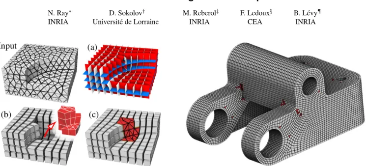
Figure 1: Left: our hexahedral-dominant meshing procedure: Start from an input tetrahedral mesh. Compute a global parameterization (a). Extract hexahedra by contouring the isovalues of the parameterization. Isolate the boundary of the void (in red), i.e., the volume with a degenerate / singular parameterization(b) (also called “gap” or “cavity”), shown in red. Remesh the void and stitch it into the hexahedral mesh(c). Right: an example of a hexahedral-dominant mesh generated by our method. This mesh contains 98% (in volume) of hexahedra. Global parameterization has filled 92.6% of the volume with hexes. An additional 5.4% was obtained by remeshing the remaining void.

Abstract

This article introduces a method to generate a hex-dominant mesh from an input tet mesh. We first compute a global parameteriza-tion, then we isolate the “void” (also called “gap” or “cavity”), that is the zone where the global parameterization is singular or too much distorted. Once properly isolated, the void can be meshed with different algorithms. Thus, our main technical contribution is an algorithm that computes the boundary of the void and makes it compatible with both the hexahedra generated in the regular part of the parameterization and the input boundary.

We tested our method on a large collection of objects (200+) with different settings. In most cases, we obtained very good quality results compared to the state-of-the-art solutions. In addition to im-proving the state-of-the-art in hex-dominant meshing, a second con-tribution of this work is to introduce a pipeline architecture, which can be used to compare present and future algorithms involved in the different steps of the pipeline (frame field generation, global pa-rameterization), for which no objective benchmark currently exists.

To ease reproducing our results and benchmarking algorithms, we provide a C++ implementation of the pipeline in the supplemental materials. ∗_{e-mail: ray@loria.fr} †_{e-mail: dmitry.sokolov@univ-lorraine.fr} ‡_{e-mail: maxence.reberol@inria.fr} §_{e-mail: franck.ledoux@cea.fr} ¶_{e-mail: levy@loria.fr}

Introduction and previous work

State of the art

Hexahedral meshing generates meshes composed of deformed cubes (hexahedra). Such meshes are often used for simulating some physics (deformation mechanics, fluid dynamics . . . ) because they can significantly improve both speed and accuracy. This is because (1) they contain a smaller number of elements (5-6 tetrahedra for a single hexahedron), (2) the associated tri-linear function basis has cubic terms that can better capture higher order variations, (3) they avoid the locking phenomena encountered with tetrahedra [Benz-ley et al. 1995], and (4) hexahedral layers can be aligned along geometric boundary features and/or some physical characteristics (flow direction, shock wave, heat gradient. . . ). Fulfilling those cri-teria required to generate hexahedral block-structured meshes. De-spite 30 years of research efforts and important advances, mainly led by Sandia National Labs in the U.S. [Tautges et al. 1996; White and Kinney 1997], generating block-structured hexahedral meshes still requires considerable manual intervention in most cases (days, often weeks for the most complicated domains). Some methods [Mar´echal 2001; Zhang and Bajaj 2004] constrain the boundary into a regular grid, but they are not fully satisfactory either, since the grid is not aligned with the boundary. In the past two decades, numerous approaches for full hexahedral meshing were proposed, geometric as well as topological. Geometric approaches comprise methods such as plastering [Blacker and Meyers 1993] and H-Morph [Owen and Saigal 2000], whereas topological approaches include whisker weaving [Tautges et al. 1996], recursive bisec-tion [Calvo and Idelsohn 2000] and dual cycle eliminabisec-tion [M¨uller-Hannemann 1999]. Unfortunately, it is very easy to find failure cases for each of these methods: all of them can fail in the termina-tion process. For geometric approaches, it typically happens when advancing fronts meet at the medial axis.

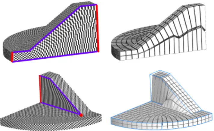
Figure 2: Left: in the presence of triangular wedges, relations be-tween constraints may create a highly distorted paramerization. Right: “HexEx” successfully constructs a valid hexahedral mesh even with such a degenerate parameterization, but clearly, the dis-torted elements still need to be fixed. Note also how the input ge-ometry was deformed (lower right).

To overcome this problem, several approaches based on global pa-rameterizations were recently proposed [Fang et al. 2016; Nieser et al. 2011]. Since they use global optimizations instead of advanc-ing fronts with local decisions, these methods do not introduce any discontinuity on the medial axis. Global optimization produces im-pressive results, but it has failure cases of its own. For the sake of completeness, we also mention the alternative approach proposed in [Gao et al. 2017], that generates a hexhaedral mesh by merg-ing tetrahedra of an input mesh along the guidance direction field. All these methods (parameterizations and agglomeration) rely on frame fields [Huang et al. 2011; Ray et al. 2016], however, no ex-isting frame-field method is guaranteed to produce an integrable 3D frame field. There were some attempts to preprocess frame fields [Li et al. 2012; Jiang et al. 2014], but unfortunately they do not address all possible issues. Locally modifying the input frame field reduces the number of failure cases, but many of them remain unsolved. Another possible option is to relax some unnecessary ex-pectations that concern the parameterization while recovering hex-ahedra, as done in [Lyon et al. 2016]. In most cases this recov-ers a correct mesh around singularities. However, as mentioned in the discussion section of [Lyon et al. 2016], some configurations cannot be handled by HexEx. In Figure 2, we show a “triangu-lar wedge”, often present in mechanical parts (see also Figure 17 P. 10 and results_02_S.pdf in the supplemental marterial). Due to the network of constraints (in blue), the two red edges are supposed to have the same length in parameter space, leading to highly stretched elements. On the bottom row, the edge in red is constrained to have the same length as the red point (i.e. zero), thus generating a single row of extremely stretched elements. Thus, it is in general not possible to extract a hex-dominant mesh of good quality from the sole parameterization. The parameterization needs to be complemented with an algorithm that isolates the distorted zones and remeshes them. Note also that HexEx deformed the ge-ometry around the degeneracy (lower-right). To avoid this behavior, a way of controlling the Hausdorff distance is also needed.

Our approach

Objective We think that given the current state of the art, aiming at full-hexahedral meshing in the general case is not realistic yet1_.

For this reason, we focus on hexahedral-dominant meshing instead

1_{with the exception of the octree-based approach in [Mar´echal 2001] that} is a robust/valid/efficient solution if boundary alignment is not required.

of full-hex, with the aim of bringing the proportion of hexahedra as near to 100% as possible.

Starting from a tetrahedral mesh, we first compute a global param-eterization. Integer iso-values of the global parameterization define a deformed grid inside the volume (Figure 1 a). It is in general not possible to extract from the parameterization a grid that fills the entire volume. Therefore, we extract hexahedra from the regu-lar part of the parameterization, as well as the boundary of the re-maining volume which have a singular/degenerate parameterization (Figure 1 b). Finally, we remesh the remaining void and stitch the meshes together (Figure 1 c). In the context of tetrahedral mesh-ing, the same approach of dividing the domain into several parts and meshing them with different algorithms resulted in significant advances. For instance, one can mesh with [George et al. 1990] the cavity that remains at the end of an advancing front method. Hex-dominant meshing will significantly benefit from a similar modular approach, but this requires to solve a non-trivial “mesh stitching” issue, addressed in this article.

This idea is not new, the CUBIT team already proposed to fill the void that remains after hex generation with tetrahedra about 20 years ago [Meyers et al. 1998]. We propose to revisit this idea in the context of recent advances of the domain: the method by Mey-ers et al. fills about 70% of the volume with hexahedra with less than 90% success ratio. We aim at bringing both the hex propor-tion and the robustness as close to 100% as possible. For this pur-pose, we combine the global structure obtained by global param-eterization approaches (e.g. CubeCover [Nieser et al. 2011] and PGP3D [Sokolov et al. 2016]) with the robustness of tetrahedral remeshing algorithms (TetGen [Si 2015]). We qualify our approach as “pragmatic”, in the meaning that we do not think that existing global parameterization approaches can solve 100% of the problem (see Figure 2). We think that in order to have a valid solution in all possible cases, global parameterization needs to be complemented with other methods in the zones where the parameterization is de-generate or undefined. As a consequence, our results are identical to the state of the art in the zones where the global parameteriza-tion successfully captures the model to be remeshed. We further improve the robustness of the overall method, by detecting and iso-lating the parts of the model that present a degenerate parameteri-zation. Then we remesh them using a different algorithm.

Our contributions

Our contribution is two-fold: we propose a robust technical solution that identifies and remeshes parts of models where the result of the global parameterization method is not satisfying. We also provide a complete testing environment that allows to compare existing frame field generation and global parameterization algorithms.

Technical solution: Global parameterization generates hexahe-dra in a large part of the input volume, that is where the parame-terization is not degenerate. The remaining void (the volume that remains to be meshed, also often called the “cavity”) conceptually corresponds to the (volumetric) boolean difference between the in-put volume and the hexahedra generated from the parameterization. The most important difficulty comes from the “stitching” issue: what we need to compute is not exactly a boolean difference, since the boundary zones that touch hex facets are remeshed as quads. Wherever the void/cavity touches the boundary, the initial bound-ary (made of triangles) needs to be connected to the quadrilateral facets of the hexahedra that touch the boundary (see Figure 4 P. 5). Another issue is that computing intersections between solid meshes is very expensive, and requires complicated data structures. In our case, this would mean computing the volumetric intersections

be-tween the input tetrahedra and the generated hexahedra (thus gen-erating polyhedra).

Our first contribution is a robust algorithm that addresses both is-sues. It computes the boundary of the void/cavity, then combines hexahedra extracted from the parameterization with a remeshing of the void. By robust, we mean that for any input tetrahedral mesh with a parameterization per tet and a manifold boundary, our solu-tion will output a mesh composed of tetrahedra and/or hexahedra. In addition, a user-specified bound on the Hausdorff distance to the input mesh can be taken into account. These guarantees are ob-tained by carefully specifying the input/output of each step, and applying only local operations that can be rolled-back in case of failure.

Testing environment: We complement this algorithm with a processing pipeline that decomposes hexahedral-dominant mesh-ing into independent steps. Existmesh-ing remeshmesh-ing algorithms as well as the corresponding software involve a long sequence of steps or-chestrated within a complicated architecture, and no existing re-search article of reasonable length can address all of them in a self-contained and complete manner. It makes it difficult to reproduce previous results, and to evaluate the impact of improving one step of the pipeline. For instance, if one wants to work on the quality of frame field generation (e.g. [Jiang et al. 2014]), it is not possible to focus on the extraction of hexahedra from the parameterization (e.g. [Lyon et al. 2016]) in the same research article.

Our open-source implementation in the supplemental material will help comparing existing and future algorithms for each step of the pipeline (3D direction field generation, global parameterization, hexahedral mesh extraction). More importantly, it will make it pos-sible to focus on each part of the pipeline independently, and to evaluate its impact on the quality of the output.

1

Overview of the hex-dominant meshing

pipeline

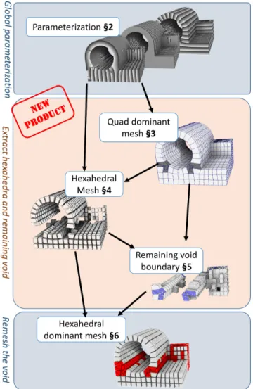
Our hexahedral remeshing pipeline is decomposed into three main steps (refer to Figures 1 and 3): compute a global parameterization (§2), generate hexahedra and extract the remaining void (§§3,4,5), and finally, remesh the void (§§5,6).

As mentioned in the previous section, the second step involves a boolean difference between two objects (the input model and the hexahedral mesh) represented by incompatible volume meshes (Figure 4). Our solution makes them compatible and avoids heavy volume remeshings by working on surfaces. The process is decom-posed into the three following steps:

• §3: we compute a quad-dominant mesh from the input bound-ary. The goal is to make it compatible with the hexahedral mesh that we compute in the subsequent step; we generate quads that are likely to match hexahedra faces. As a repre-sentation of the object volume, the quad-dominant mesh must be closed, manifold and free of self-intersection, i.e. a valid input for a 3D constrained Delaunay triangulation algorithm2; • §4: we extract the hexahedra from the pre-image of the param-eterization (i.e., the deformed grid shown in Figure 1 a). From this set of hexahedra, we remove the elements that would not produce a valid hexahedral mesh, or that intersect the quad-dominant mesh of the boundary;

• §5: we compute the boolean difference between the surface of the hexahedral mesh and the quad-dominant mesh of the boundary. Since the boundary is compatible with the quad

2_{in the results presented here we used Tetgen [Si 2015].}

Figure 3: Overview of the pipeline with the result of each step. facets of the hexahedra, the boolean difference is no longer a geometric operation, it becomes purely combinatorial.

Robustness Our process is robust, in the sense that it always outputs a 3D mesh composed of hexahedra and/or tetrahedra with a bounded symmetric Hausdorff distance to the data. We preserve some properties of the mesh throughout all the processing steps, as summarized below and detailed later:

The input tet mesh has no self-intersection and has a manifold boundary. The parameterization step computes a triplet of coor-dinates associated with each tetrahedron corner. The tetrahedron faces with a singular or too much distorted parameterization are marked as invalid. The quad-dominant mesh is produced by iter-atively modifying the input boundary with local operations, while preserving the absence of self-intersection. The hexahedral mesh is extracted from the parameterization. We only keep the hexa-hedra that are free of intersection with other hexahexa-hedra, and that are located inside the new (quad-dominant) boundary mesh. The boundary of the remaining void is composed of the hexahedral mesh boundary and the quad dominant mesh, therefore it has no self-intersection. At this step, it is possible to fill the void with a constrained tetrahedrization, that is finally combined with the hex-ahedral mesh.

The difficulties are to ensure that the algorithm terminates, that the result is intersection-free and within bounded Haussdorff distance to the data. This is done by carefully orchestrating the detection of

the new intersections possibly introduced by the generated quads.

2

Global parameterization

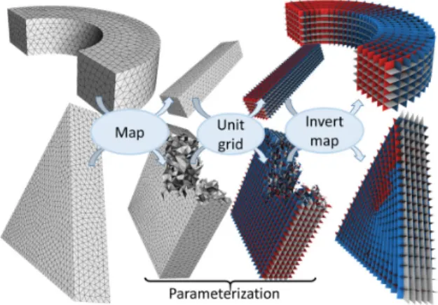
A global parameterization [Gregson et al. 2011; Nieser et al. 2011; Li et al. 2012; Sokolov et al. 2016; Fang et al. 2016] is a map that deforms a solid object in 3D space. Consider the unit grid in the parameter space and project it onto the object space using the in-verse of the deformation map, we can get a hexahedral mesh of the object (see Figure 5 P. 5, upper row). In simple cases, the parame-terization is a continuous map (e.g. in [Gregson et al. 2011]), but it can be also discontinuous, as was shown in [Nieser et al. 2011; Li et al. 2012]. If this discontinuous map satisfies “grid compatibility” constraints, then it can still produce a nice hexahedral mesh (see Figure 5, bottom row).

To generate a global parameterization, the main difficulty is to de-termine where to place the singularities i.e. the points of the volume where the pre-image of the unit grid is not a deformed grid. A com-mon strategy is to compute a frame field that places some of these singularities, then to optimize a grid-compatible map guided by the frame field. In §7.2, we compare different solutions for both steps. The output of the global parameterization is a set of local linear maps attached to (a subset of) the tetrahedra. In general, the param-eterization is supposed to satisfy the grid-compatibility constraint between each pair of adjacent tetrahedra. This constraint allows our method to generate hexahedra that overlap several tetrahedra. In contrast to previous works [Lyon et al. 2016], our method is ro-bust to parameterizations that do not satisfy the grid-compatibility constraint everywhere.

3

Quad dominant mesh of the boundary

Our central technical contribution is an algorithm that computes the boundary of the void left by the global parameterization. As we explained in the introduction, it requires to make the bound-ary mesh compatible with the quad facets of the generated hexahe-dra in zones where the void and the generated hexahehexahe-dra touch the boundary (see Figure 4). This section explains how to enforce this compatibility.

The input of our algorithm is a tetrahedral mesh T with: a 3D global parameterization given by a (u, v, w) triplet attached to each tet corner, and a boolean flag per tet facet that indicates whether the facet has a valid parameterization.

The output is a quad-dominant remeshing of the boundary ∂T , that is a closed manifold surface free of self-intersection (i.e., a valid input for a 3D constrained Delaunay triangulation). In more de-tails, since 3D constrained Delaunay triangulations in general do not support quads as input constraints, we ensure that all possible triangulated surfaces obtained by splitting each quad into two tri-angles is free of self-intersections. Moreover, we can (optionally) ensure that the Hausdorff distance between ∂T and the quad domi-nant mesh is smaller than a given threshold.

Algorithm: The input boundary ∂T is originally free of self-intersections. Therefore, it can be considered as a valid (though not very interesting !) output. Our algorithm starts with this surface and transforms it into a compatible quad-dominant mesh by apply-ing a series of local operations. Robustness is ensured by checkapply-ing after each operation (steps 2 and 4), that the surface is still free of self-intersections. Whenever an intersection is detected, the opera-tions that created the intersection are detected, the region where the intersection occured is locked (in a sense that will be detailed later),

and the entire step is restarted. The process terminates as soon as the result is free of self-intersections.

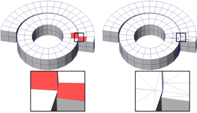
Our solution may look like using a sledge-hammer to crack a nut, but proving the robustness of simpler approaches is indeed much more difficult. For instance, directly extracting quads from the pa-rameterization as in QEx/HexEx is not completely safe (Figure 7), and the algorithm that will have to remesh the rest of the surface will still face the same robustness issues as us . . . plus it will have to support a constrained boundary due to quad edges.

The whole quad-dominant remeshing algorithm is illustrated in Fig-ure 6 and detailed in the rest of this section:

Figure 6.1:Extract the input surface ∂T and its 2D parame-terization (§3.1);

Figure 6.2:create extra edges that are likely to match hexahe-dra edges (§3.2);

Figure 6.3:create charts of facets that correspond to the facets we want to create in the quad-dominant mesh, i.e. a set of quads that are likely to match a hexahedron facet (§3.3), or the original triangles elsewhere;

Figure 6.4: simplify the mesh by tentatively merging the facets that belong to the same chart. The (optional) control of the Hausdorff distance is performed during this step.

3.1 Extract the 2D parameterization of the boundary from the 3D parameterization

The 2D parameterization is defined as a restriction of the 3D pa-rameterization to a subset of the boundary triangles. If exactly one coordinate has a constant integer value on a triangle, then the pa-rameterization is defined on this triangle by the two other coordi-nates, else the triangle is flagged as invalid.

Figure 6-input shows three input scalar fields. The facets with an invalid 3D parameterization are shown in blue. The 2D parame-terization Figure 6-1 has a valid 2D parameparame-terization whenever it is drawn in red exactly once in the “Input” figure. The group of two triangles in blue is invalid because one was aready marked as invalid in the 3D parameterization, and the triangle in the corner (figure 6-1, marked by an arrow) is invalid because it has no con-stant iso-integer coordinate (never marked in red in the input). Note that our 2D parameterization inherits the grid-compatibility of the 3D parameterization (that may or may be not be satisfied, with or without numerical imprecisions). Note also that axes can be switched in pairs of adjacent triangles.

3.2 Create new edges

We recall that our goal is to create quads that are likely to corre-spond to edges of the hexahedra extracted from the 3D parameter-ization. We first create the edges of the quads, by imprinting the integer isovalues of the 2D parameterization. They appear as new edges, created by splitting the facets. This step is decomposed into two substeps (split the edges, split the facets), as illustrated in fig-ure 6-2. As vertices coordinates are represented by floating point numbers, this operation may produce self-intersections due to nu-merical imprecisions. Therefore, this step requires a rolling-back strategy.

Split the edges The first substep computes the intersection of the imprinted isoparametric lines with the edges of the original tri-angular mesh ∂T and creates the corresponding vertices. The left

Figure 4: Left: boundary of the hexahedral mesh. Middle: incom-patibility with the input boundary (blue). Right: comincom-patibility with our quad dominant remeshing (blue).

Figure 5: Upper row: A map deforms an input object (left) to align its normals with the(x, y, z) axis (middle–left). A regular grid (middle–right) defined on the image of the object can be deformed to match the original object using the invert function.Lower row: a global parameterization accepts a larger, more relaxed class of maps (grid preserving), that may include some discontinuities.

Figure 6: Compute a quad-dominant mesh of the input boundary. (1) Restrict the 3D parameterization to 2D; (2) imprint the integer isovalues of the parameterization into the mesh;(3) (left) regroup facets into charts separated by iso-values ; (middle) restore charts corresponding to the original triangulation in non-quad zone (red dotted area) ; (right) remove unnecessary constraints from the quad-triangles interface.(4) simplify the mesh w.r.t to the charts, producing the output quad-dominant mesh.

Figure 7: Remeshing concentric curved features may generate new intersections in the created primitives (left–red quads). Our algo-rithm detects them and keeps the original mesh in the concerned zones (right).

image of Figure 6-2 shows the resulting polygonal mesh. The blue vertices were added by splitting the edges. The original vertices are marked in green.

The algorithm that generates these new vertices works as follows: for each edge, we choose one of its neighboring polygons with a valid parameterization (if it exists) and use its parametric coordi-nates to split the edge. To do so, we compute all points of the edge that have at least one integer coordinate in the parametric domain. We sort these points by growing distance from one edge extremity, and insert them in the edge. The parametric coordinates are then evaluated from the linear map defined in each polygon.

Robustness:We do not assume that this step will introduce all ver-tices, nor that they will be sorted correctly, nor that the coordinate that is supposed to be integer is indeed integer. The only require-ment is that all coordinates (geometric and parametric) are valid floating-point numbers.

Implementation details:Our implementation uses standard double-precision floating point numbers. We do not create vertices with invalid coordinates. Also, coordinates that are closer than 10−10 to their nearest integer are snapped to this integer. This snapping is not mandatory for robustness, but it allows to miss a smaller number of iso-integer value edges: it accounts for numerical imprecisions during the evaluation of parametric coordinates, including when the transition function is not exactly grid-preserving.

Split the facets We iteratively split facets by creating a new edge between a pair of vertices having a common integer parametric co-ordinate. The new edge is split by inserting new vertices at integer values of the other coordinates. This process creates edges along each integer isovalues, and introduces vertices at the intersections of integer isovalues, as illustrated in Figure 6-2 (right image, red vertices). Once all facets are split, we triangulate the facets. Before splitting a facet, we check that:

• the new edge does not connect two successive vertices of the polygon (would produce a facet with 2 vertices),

• and, in parametric space, all the vertices of the new facets are located in the opposite half planes separated by the cut (except the extremities of the cut).

These conditions are required to ensure that the algorithm termi-nates. To prove that the algorithm converges, one can consider the number of created vertices at each step of the algorithm: all created vertices have integer coordinates and are located in the bounding box of the current vertices. The number of vertices is necessar-ily lower in both half polygons than in the original polygon, thus

the number of created vertices is a strictly decreasing sequence of integers. At the end of the process, the surface is triangulated to ease computing intersections (rollback substep) and vertex removal (simplification step).

Rollback Before starting the next step, we test whether the sur-face is free of self-intersections. We recall that the original mesh was free of intersections, thus intersections are created when split-ting the facets with the iso-parametric lines. If intersections are detected, we restore the original mesh and, for each facet that has an intersecting facet in its decomposition (obtained when splitting it), we flag it as having no valid parameterization. The effect of flagging the facets that yielded intersections is that they will be no longer split. We then restart the process until no more self-intersection is produced.

3.3 “Paint” the desired new mesh

Recall that the objective of this section is to produce an intersection-free mesh that has: quad facets where the parameterization is valid, the original triangles everywhere else, and a valid mesh at the junc-tion of these regions.

Thanks to the imprint realized by the previous step, both the quads and the original triangles can be represented as groups of facets (that we call “charts”). The present step determines these charts as follows (Figure 6-3):

• find quads: We create one chart per facet then, for each pair of adjacent facets, we merge their charts if both have a valid parameterization and are not separated by an isovalue edge. We consider that a chart corresponds to a quad if its boundary solely contains isovalue edges and if it has 4 iso-value corners. At this step, we can optionally filter quads that are not flat or too distorted;

• find triangles: We create a chart per quad detected earlier, and a chart per facet not included in one of these quads. For each pair of adjacent facets, we merge their charts if they where produced from the same triangle of the original surface ∂T ;

• relax the triangle constraint: For each pair of adjacent facets, we merge their charts if they are not separated by an isovalue edge, and have one extremity located on a quad chart boundary. This step allows the mesh simplification algorithm to modify the original geometry nearby the quads.

3.4 Simplify the mesh

The objective here is to replace as many charts as possible by their corresponding facet. To do so, we visit each vertex that is not a quad corner, and try to remove it according to the number of charts it touches:

• 1 chart: we remove the incident fan of triangles and late the hole (our implementation uses a min-weight triangu-lation);

• 2 charts: we remove the incident fan of triangles and triangu-late the hole with the constraint that one edge should follow the chart boundary;

• 0 or more than 2 groups: we do not remove the vertex. At the end of the process, most quad charts are represented by two triangles, and most original triangles that do not participate to quad charts are represented by a single triangle.

Figure 8: The quad dominant mesh computed from the input mesh (left) without (middle) and with (right) control of the symmetric Hausdorff distance.

Rollback During the simplification, we associate to each new facet the Id of the vertex that is being removed. When the sim-plification is done, we test the new surface for self-intersections. If two triangles intersect, we restore the original surface and lock their corresponding vertices. The simplification is performed once again, until all self-intersections are removed.

Note that a quad may be triangulated in two possible ways. Since we do not know at this step how they will be triangulated, we test both configurations for intersections.

Controlling the Hausdorff distance We ensure (Figure 8) that the symmetric Hausdorff distance between the boundary of the gen-erated mesh and the boundary of the original mesh ∂T is lower than a user-defined ε by locking additional vertices before the rollback. The locked vertices are either the vertices that produced a facet of the new mesh with a point that is too far away from ∂T , or the three vertices of the triangle of ∂T with a point that is too far away from the new mesh. To evaluate an upper bound of the Hausdorff dis-tance, we sample each facet in such a way that each point of the facet is closer than ε/2 to a sample, then we compute the distance between each sample and the other mesh. If this distance is greater than ε/2, the Hausdorff distance may be greater than ε, so the facet is considered as being too far away.

4

Hexahedral mesh

We extract the hexahedra from the parameterization as in [Nieser et al. 2011]. In addition, we filter them to prevent producing an in-valid boundary of the void. The filtering strategy starts by merging vertices with the same coordinates (up to a numerical precision er-ror), then we discard each hexahedron that have an intersection with the quad-dominant mesh or another hexahedron, and where this in-tersection does not perfectly match a vertex, an edge or a quad (Fig-ure 10). A quad is considered as intersecting another facet if one of its two possible triangulations is intersecting it.

In Figure 9–left, two red hexahedra share three vertices of the same facet: it is considered as an intersection because there exists a tri-angulation of both hexahedra facets that shares a triangle (defined by shared vertices). We can also optionally filter hexahedra based on geometric criteria, such as with a threshold on dihedral angles (Figure 9–right).

Another case of intersection is the red hexahedra in Figure 10– Right. They have facets that intersect the boundary of the

quad-Figure 9: Invalid configurations: hexahedra sharing 3 vertices (left) and badly shaped hexahedron (right).

Figure 10: The quad-dominant mesh (on the left) does not match the facets of the red hexahedra, therefore these hexahedra need to be removed.

dominant surface (Figure 10–Left).

5

Void boundary

We define the boundary of the void volume as the difference be-tween the quad-dominant mesh and the boundary of the produced hexahedra. At this stage, the quad-dominant mesh of the boundary and the extracted set of hexahedra are both free of intersection and compatible (the quad faces and hexahedra faces match), therefore the boolean operation that is required to compute the boundary of the cavity boils down to a purely combinatorial operation, and this step is straightforward to implement (in a certain sense, all difficul-ties have been pushed towards the previous steps).

6

Hexahedral dominant mesh

As previously mentioned and summarized in Figure 3, the purpose of this article is to define and extract the remaining void, not to remesh it: this is left to existing or future algorithms. We first show results where the remaining void is filled by a constrained Delau-nay triangulation (here TetGen) to demonstrate that the boundary mesh computed by our algorithm is valid. Then we show two al-ternatives to further improve the proportion of hexahedra in the void, and compare the so-obtained results with other hexahedral-dominant meshing methods (Figure 18). The first one (see §6.1 for more details) is a robust solution inspired by [Carrier-Baudouin et al. 2014], and the second one (§6.2) is a more complicated com-bination of previous works that achieve better performances at the expense of robustness (it did not work on all examples).

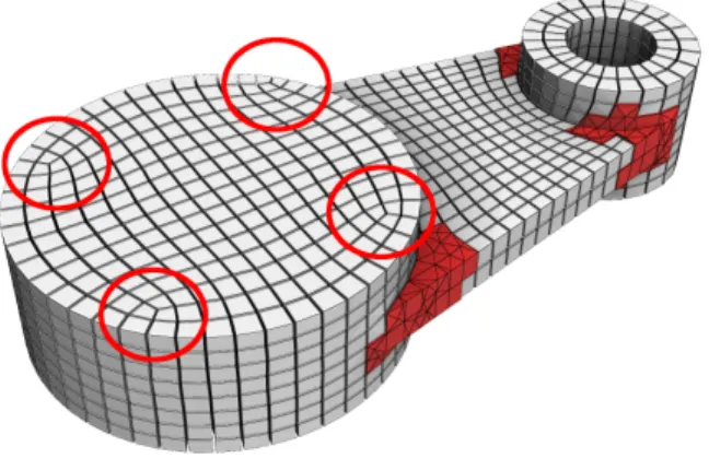
Better solutions should probably take into account the specific structure of the remaining void. Our preliminary results in this di-rection (Figure 11) seem to be encouraging. We expect future works to compete with [Li et al. 2012] and [Lyon et al. 2016] for models that can be remeshed with hexahedra only. The remaining void that corresponds to the singularities of the frame field is particular in the sense that it exhibits a structure that can often be completely filled with hexahedra (or prisms). Note that they could be avoided in the first place by applying the original CubeCover algorithm, but it comes with its own drawbacks (lack of degrees of freedom and

Figure 11: Cavities due to frame field singularities (circled) can often be filled by a full hexahedral mesh.

needs for constrained singularity [Li et al. 2012] or robust extrac-tion of hexahedra [Lyon et al. 2016]).

6.1 Void filling alternative # 1: merge tetrahedra into hexahedra

This algorithm is inspired by the final step of [Carrier-Baudouin et al. 2014]. It fills a volume with a point set, remeshes the vol-ume with tetrahedra, and recombines them into hexahedra where possible. It inherits the robustness of the original algorithm, but cannot reproduce its performances due to our strongly constrained boundary.

6.2 Void filling alternative # 2: classic hexahedral meshing

The void can also be filled by more classic algorithms: quad-paving[White and Kinney 1997] and whisker-weaving [Tautges et al. 1996]: We first increase the proportion of quads by apply-ing quad pavapply-ing to all the triangulated patches of the void bound-aries. Then, we iteratively remove layers of hexahedra (and prisms) with whisker weaving. We only allow to remove layers that have one side completely included inside the boundary of the void. This strategy peels the object one layer at a time, and directly produces hexahedra and prisms by extruding the quads and triangles of the void boundaries. At the end of the process, if tetrahedra remain in the void, we fallback to the other algorithm (tetrahedron merging §6.1).

7

Results and analysis

In this section, we compare our results with previous works §7.1, and we demonstrate that our pipeline makes it possible to compare different implementations of each step §7.2. We experimented with our algorithm on a database of 200+ models, the reader can refer to the supplemental material for the complete list, images and hex-proportion statistics. General trends are summarized and analyzed below.

The running times are summarized in Figure 13: the whole process takes a couple of minutes for objects with hundreds of thousands tetrahedra, and up to half an hour for tens of millions tetrahedra.

Figure 12: The mesh boundary produced by PGP3D [Sokolov et al. 2016] depends on a parameter that may miss some parts (left) or produce useless tetrahedra (middle). Our method is not subject to these problems (right).

0 ₁₀4 ₁₀5 ₁₀6 ₁₀7 0 101 102 103 104

Frame fields generation Global parameterization Quad dominant remeshing Extracting hexahedra Remaining void boundary Filling the void

nb input tets time (s.)

Figure 13: Timings (in seconds) for each step of the pipeline in function of the number of tetrahedra in the input mesh (log/log scale).

Figure 14: Distribution of the proportion of volume filled by hex-ahedra for all the 200+ models of the database (horizontal axis: proportion of hexahedra, vertical axis: number of models). In the first column, the frame field is obtained by solving a linear system. In the second column it is further optimized with non-linear iter-ations. The rows correspond to the global parameterization algo-rithm: Cubecover, PGP3D with curl correction, and PGP3D with-out curl correction respectively.

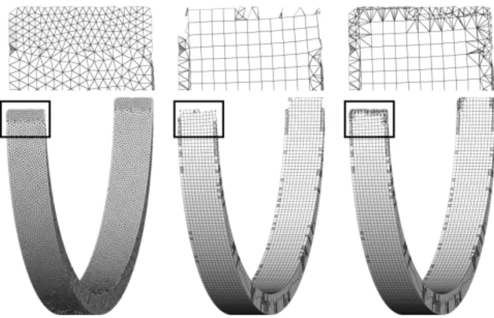
Figure 15: We preserve geometric details with tetrahedra. Cube-cover and its extensions cannot directly handle them.Top row: di-rect tetrahedralization of the remaining void,bottom row: paving + whisker weaving used to fill the void (refer to§6.2).

7.1 Comparison with previous works

Hexahedral dominant remeshing using frame fields provides inter-esting results [Carrier-Baudouin et al. 2014], but global optimiza-tion of the frame field and vertex posioptimiza-tioning improves the results [Sokolov et al. 2016]. Our method differs from the latter solution on the following aspects:

• we obtain a more faithful mesh boundary: it is either the orig-inal mesh or the deformed grid, whereas [Sokolov et al. 2016] re-samples the surface and introduces new points until a Haus-dorff distance criterion is met. Figure 12 shows that the results are sensitive to the distance threshold;

• hexahedra are directly extracted from the parameterization rather than recombined from a tetrahedral mesh generated from a point cloud. It prevents extracting isolated hexahedra and mismatches that occur in [Sokolov et al. 2016, Figure. 20] when the parameterization is too much distorted;

• our pipeline can use CubeCover for computing the parame-terization. For meshes without incompatible constraints, this leads to drastic improvements in terms of mesh quality. This point is further discussed in §7.2.2;

We compare the proportion of hexahedra obtained by our method and by PGP3D[Sokolov et al. 2016] in table 1. Our results are presented with the remaining void remeshed by the two robust so-lutions we have: TetGen and the algorithm derived from [Carrier-Baudouin et al. 2014]. We observe that the latter algorithm gives the best results, even without exploiting the specific structure of the remaining void. We think that doing so will probably further im-prove the results.

Note on full hexahedral remeshing If a shape can be remeshed with a full hexahedral mesh extracted from a global parameteriza-tion [Nieser et al. 2011; Li et al. 2012; Lyon et al. 2016], clearly our solution will not be better than a 100% full-hex mesh that it generates. However in practice, most models cannot be com-pletely remeshed by such a method, due to globally incompatible constraints, or geometric details that are hard to capture with a de-formed grid of hexahedra (some examples are shown in Figure 15).

model our method our method PGP3D +TetGen only +Carrier-Baudoin

fusee 92.9 95 94.6 CV745 92.3 94.4 91.6 propeller 85.1 89.4 91.1 cubo 88.8 91.8 89 cylinder 98.9 99.3 90.9 corner 99.3 99.7 99.5 fandisk 75.5 82.6 77.8 impeller 73.3 81.8 81.1 bunny 89.8 92.2 88.6 bone 70 81.9 82.54 fertility 79.9 86.4 78.4

Table 1: Proportion of volume filled by hexahedra (in %). First two columns: our method using two strategies to fill the voids (TetGen, and [Carrier-Baudouin et al. 2014]). Right column: comparison with PGP3D results (reported in [Sokolov et al. 2016]).

7.2 Using our pipeline to compare previous works

Another benefit of our contribution is the pipeline that makes it easy to evaluate the impact of each step on the quality of the results. This section demonstrates its usefulness by comparing different options for the steps that can be implemented by previous works: frame field, parameterization, and remeshing the remaining void.

7.2.1 Frame field optimization

We compute frame fields with [Ray et al. 2016] that proposes two options: the first one requires only solving a least-squares problem, and the second one further improve this initialization with a non-linear optimization.

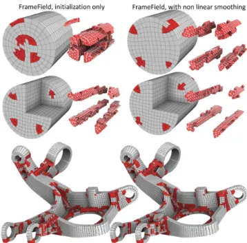
The influence of each solution is presented in the columns of Fig-ure 14. We observe that it does not really impact the result’s qual-ity, except for a few models that really need the non-linear opti-mization. It confirms the observation done in [Ray et al. 2016] that the non-linear optimization is mandatory for objects of revolution (cylinders), but it is less important for other models (Figure 16).

7.2.2 Parameterization

Our default implementation runs [Nieser et al. 2011] on the mesh minus the frame field singularities (defined as in [Ray et al. 2016]). Not including frame field singularities makes it easier to implement, and offers more degrees of freedom around singulari-ties that are not compatible with hexahedral remeshing. We com-pare it to PGP3D [Sokolov et al. 2016] with or without the optional curl correction.

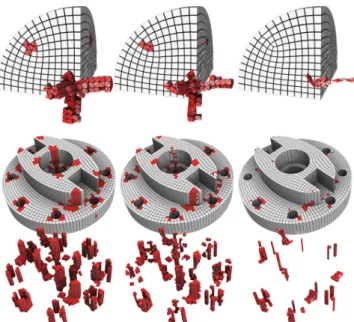
The performance of each algorithm is compared in the rows of Fig-ure 14. The distribution of hexahedra on the model is very differ-ent with each solutions (Figure 17): CubeCover may produce large remaining voids whereas PGP3D evenly distributes them over the mesh.

7.2.3 Filling the void

The algorithms that fill the remaining void are compared in Fig-ure 19, and an example is given in FigFig-ure 18. We observe that the proportion of hexahedra can be significantly improved when remeshing the remaining void. This adaptation of existing algo-rithms already provides better results than the state of the art. We think that even better results could be obtained with more special-ized algorithms, that we will study in future works.

Figure 16: Impact of frame fields computed without (left column) or with (right column) the non linear part of the optimization. For the cylinders (top row), the remaining tetrahedra are visualized alone, to better reveal the inner structure.

Figure 17: Two shapes remeshed by CubeCover, PGP3D with curl correction and PGP3D without curl correction.

Figure 18: Hexahedral dominant meshes obtained by remeshing the void with (from left to right) TetGen, our adaptation of [Carrier-Baudouin et al. 2014], and our paving + whisker weaving imple-mentation. To better visualize the mesh inside the volume we also show the tetrahedra separately.

Figure 19: Hex proportion (in volume) gained when remeshing the void using two different strategies. The horizontal axis corresponds to the hex proportion obtained from the non-singular zones of the parameterization, and the vertical axis to the final hex proportion. We compare our adaptation of [Carrier-Baudouin et al. 2014] (red dots) and paving+whisker-weaving (blue dots). In general, when successful, paving + whisker-weaving better increases the hex pro-portion, but is less robust (we observed many failure cases).

8

Conclusion

This work does not solve full-hexahedral meshing, but we think it realizes a significant step forward, and opens several interesting re-search avenues. Besides the improvements that we obtained in the quality of the results, our pipeline architecture helps benchmark-ing existbenchmark-ing algorithms, and evaluatbenchmark-ing the quality of frame fields. It lets global parameterization algorithms focus on capturing the global shape. Remeshing the remaining void is also an interesting challenge: the problem is a special case of boundary-constrained hexahedral meshing. The modular nature of our algorithm and the possibility of respecting boundary constraints also gives additional possibility of plugging-in specialized algorithms for meshing par-ticular geometries, such as fillets or tubular structures.

Evaluation is another topic that will require further work. For now, in the context of this article, we used for the evaluation the pro-portion of generated hexahedra, constrained to have a metric tensor condition number smaller than 10 (see §3.1). While it gives rea-sonably shaped elements, we think that a more thorough evaluation will be needed in the future, where the meshes are evaluated in the context of FEM (Finite Element Modeling) simulations. It would be important to compare the impact of the mesh on both the accu-racy of the solution and speed of the simulation. Setting-up such an experiment requires a substantial amount of work, well beyond the scope of this article. It may be considered as a first step towards this direction, by providing an automatic and reproducible pipeline for the mesh generation part.

References

BENZLEY, S. E., ERNEST PERRY, K., MERKLEY, B. C., AND

SJAARDEMA, G. 1995. A comparison of hexahedral and all-tetrahedral finite element meshes for elastic and elasto-plastic analysis. In International Meshing Roundtable conf. proc. BLACKER, T. D.,ANDMEYERS, R. J. 1993. Seams and wedges

in plastering: A 3-d hexahedral mesh generation algorithm. En-gineering with Computers 9, 2, 83–93.

CALVO, N. A.,ANDIDELSOHN, S. R. 2000. All-hexahedral ele-ment meshing: Generation of the dual mesh by recurrent subdivi-sion. Computer Methods in Applied Mechanics and Engineering 182, 3–4, 371 – 378.

CARRIER-BAUDOUIN, T., REMACLE, J.-F., MARCHANDISE, E., HENROTTE, F.,ANDGEUZAINE, C. 2014. A frontal approach to hex-dominant mesh generation. Advanced Modeling and Sim-ulation in Engineering Sciences 1, 1.

FANG, X., XU, W., BAO, H., AND HUANG, J. 2016. All-hex meshing using closed-form induced polycube. ACM Trans. Graph. 35, 4 (July), 124:1–124:9.

GAO, X., JAKOB, W., TARINI, M.,AND PANOZZO, D. 2017. Robust hex-dominant mesh generation using field-guided poly-hedral agglomeration. ACM TOG (SIGGRAPH conf. proc.). GEORGE, P., HECHT, F.,ANDSALTEL, E. 1990. Fully automatic

mesh generator for 3d domains of any shape. IMPACT Comput. Sci. Eng. 2, 3, 187–218.

GREGSON, J., SHEFFER, A., AND ZHANG, E. 2011. All-hex mesh generation via volumetric polycube deformation. Com-puter Graphics Forum (Special Issue of Symposium on Geometry Processing 2011) 30, 5, to appear.

HUANG, J., TONG, Y., WEI, H.,ANDBAO, H. 2011. Boundary aligned smooth 3d cross-frame field. ACM Trans. Graph. 30, 6 (Dec.), 143:1–143:8.

JIANG, T., HUANG, J., WANG, Y., TONG, Y.,ANDBAO, H. 2014. Frame field singularity correction for automatic hexahedraliza-tion. IEEE Transactions on Visualization and Computer Graph-ics 20, 8, 1189–1199.

LI, Y., LIU, Y., XU, W., WANG, W.,ANDGUO, B. 2012. All-hex meshing using singularity-restricted field. ACM Trans. Graph. 31, 6 (Nov.), 177:1–177:11.

LYON, M., BOMMES, D.,ANDKOBBELT, L. 2016. HexEx: Ro-bust hexahedral mesh extraction. ACM Trans. Graph..

MARECHAL´ , L. 2001. A new approach to octree-based hexahedral meshing. In International Meshing Roundtable conf. proc. MEYERS, R. J., TAUTGES, T. J., TUCHINSKY, P. M., AND

TUCHINSKY, D. P. M. 1998. The ”hex-tet” hex-dominant mesh-ing algorithm as implemented in cubit. In in CUBIT; Proceed-ings, 7 th International Meshing Roundtable 98, Sandia National Laboratories, 151–158.

M ¨ULLER-HANNEMANN, M. 1999. Hexahedral mesh generation by successive dual cycle elimination. Engineering with Comput-ers 15, 3, 269–279.

NIESER, M., REITEBUCH, U.,ANDPOLTHIER, K. 2011. Cube-cover– parameterization of 3d volumes. Computer Graphics Fo-rum 30, 5, 1397–1406.

OWEN, S. J.,ANDSAIGAL, S. 2000. H-morph: an indirect ap-proach to advancing front hex meshing. International Journal for Numerical Methods in Engineering 49, 1-2, 289–312. RAY, N., SOKOLOV, D.,ANDL ´EVY, B. 2016. Practical 3d frame

field generation. ACM Trans. Graph. 35, 6 (Nov.), 233:1–233:9. SI, H. 2015. Tetgen, a delaunay-based quality tetrahedral mesh

generator. ACM Trans. Math. Softw. 41, 2 (Feb.), 11:1–11:36. SOKOLOV, D., RAY, N., UNTEREINER, L., AND L ´EVY, B.

2016. Hexahedral-dominant meshing. ACM Trans. Graph. 35, 5 (June), 157:1–157:23.

TAUTGES, T. J., BLACKER, T.,ANDMITCHELL, S. A. 1996. The whisker weaving algorithm: A connectivity-based method for constructing all-hexahedral finite element meshes. International Journal for Numerical Methods in Engineering 39, 19, 3327– 3349.

WHITE, D. R.,ANDKINNEY, P. 1997. Redesign of the Paving Algorithm: Robustness Enhancements through Element by Ele-ment Meshing. In Proceedings of the 6th Iternational Meshing Roundtable, 323–335.

ZHANG, Y.,ANDBAJAJ, C. 2004. Adaptive and quality quadrilat-eral/hexahedral meshing from volumetric data. In International Meshing Roundtable conf. proc.