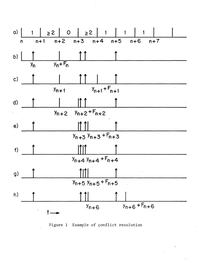
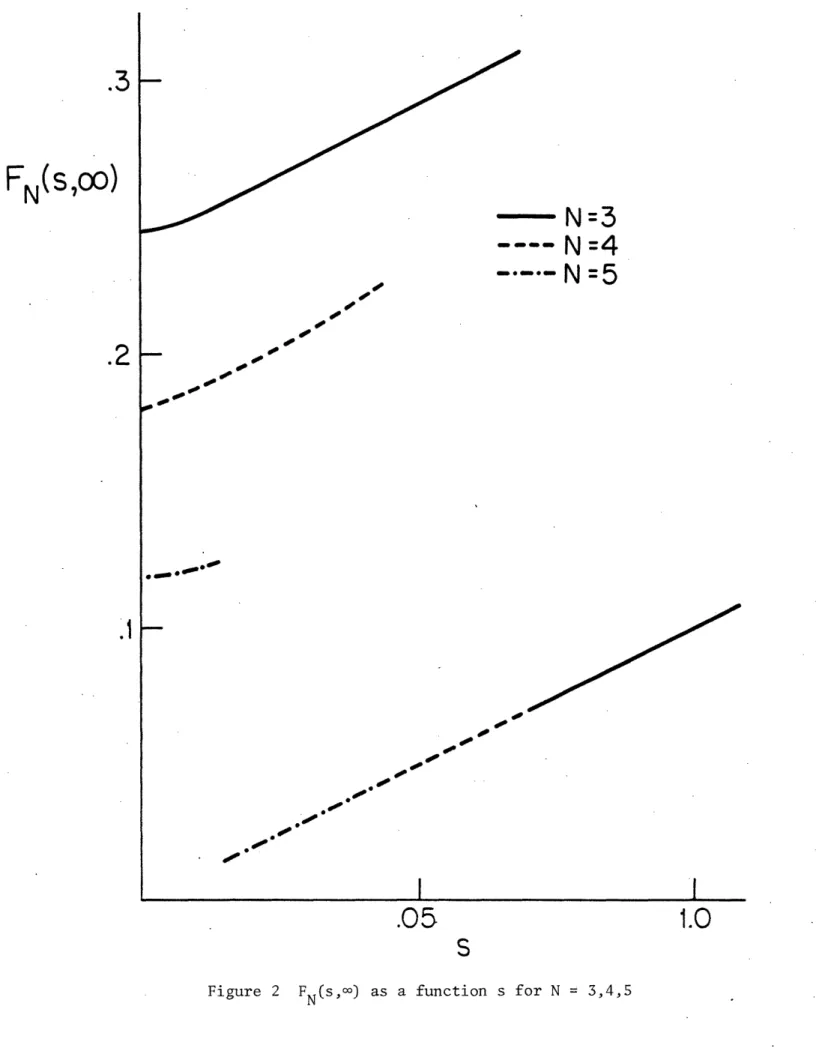
A class of efficient contention resolution algorithms for multiple access channels

Before the additional provision of 550 million euro recorded for the first half of 2009 against the Finnish OL3 contract, operating income amounted to 566 million euro, representing

TORREA, Weighted and vector-valued inequalities for potential operators. 295 (1986),

This approach is attractive in certain contexts (e. Beurling's interpolation theorem [7]. Beurling's theorem is intimately connected with the construction of our

Total revenues Service revenues thereof mobile service revenues thereof fixed-line service revenues Equipment revenues Other operating income EBITDA % of total revenues EBIT..

Group total costs and expenses rose by 2.5% year-on-year to EUR 742.9 mn in the second quarter of 2018 reported: +2.7%, mainly driven by higher cost of equipment, increased

In the Belarusian segment, EBITDA rose by 24.1% reported: +28.0% on a local currency basis in the first half of 2017 compared to the same period last year, as the increase in

In the second quarter of 2016, Telekom Austria Group results benefitted mostly from strong operations in Austria, with additional support from the demand for data-centric services

As a result of higher revenues and lower operating expenses, EBITDA comparable rose by 6.1% year-on-year in the second quarter of 2015 excluding the above mentioned