HAL Id: hal-02362956
https://hal.archives-ouvertes.fr/hal-02362956
Submitted on 14 Nov 2019HAL is a multi-disciplinary open access archive for the deposit and dissemination of sci-entific research documents, whether they are pub-lished or not. The documents may come from teaching and research institutions in France or abroad, or from public or private research centers.
L’archive ouverte pluridisciplinaire HAL, est destinée au dépôt et à la diffusion de documents scientifiques de niveau recherche, publiés ou non, émanant des établissements d’enseignement et de recherche français ou étrangers, des laboratoires publics ou privés.
Modelling methane hydrate stability changes and gas
release due to seasonal oscillations in bottom water
temperatures on the Rio Grande cone, offshore southern
Brazil
R. Braga, R.S. Iglesias, C. Romio, D. Praeg, D.J. Miller, A. Viana, J.M.
Ketzer
To cite this version:
R. Braga, R.S. Iglesias, C. Romio, D. Praeg, D.J. Miller, et al.. Modelling methane hydrate sta-bility changes and gas release due to seasonal oscillations in bottom water temperatures on the Rio Grande cone, offshore southern Brazil. Marine and Petroleum Geology, Elsevier, 2020, 112, pp.104071. �10.1016/j.marpetgeo.2019.104071�. �hal-02362956�
1
MODELLING METHANE HYDRATE STABILITY CHANGES AND GAS RELEASE DUE TO SEASONAL OSCILLATIONS IN BOTTOM WATER TEMPERATURES ON THE RIO GRANDE CONE, OFFSHORE SOUTHERN BRAZIL
R. Braga1; R. S. Iglesias1,3*; C. Romio2;D. Praeg1,4; D.J. Miller5, A.; Viana6; J.M. Ketzer7
1 Instituto do Petróleo e dos Recursos Naturais – PUCRS – Pontifícia Universidade Católica do Rio
Grande do Sul, 90619-900, Porto Alegre, RS, Brazil
2 Department of Engineering - Biological and Chemical Engineering, Aarhus University, 8200 Aarhus,
Denmark
3 Escola Politécnica – PUCRS – Pontifícia Universidade Católica do Rio Grande do Sul, 90619-900,
Porto Alegre, RS, Brazil
4 Géoazur, UMR7329 CNRS, 250 Rue Albert Einstein, 06560, Valbonne, France
5 PETROBRAS - CENPES Centro de Pesquisas e Desenvolvimento Leopoldo Américo Miguez de
Mello, 21941-915, Rio de Janeiro, RJ, Brazil
6 PETROBRAS E&P, 20031-912, Rio de Janeiro, RJ, Brazil
7 Department of Biology and Environmental Science, Linnaeus University, 391 82, Kalmar, Sweden.
2
ABSTRACT
The stability of methane hydrates on continental margins worldwide is sensitive to changes in temperature and pressure conditions. It has been shown how gradual increases in bottom water temperatures due to ocean warming over post-glacial timescales can destabilize shallow oceanic hydrate deposits, causing their dissociation and gas release into the ocean. However, bottom water temperatures (BWT) may also vary significantly over much shorter timescales, including due to seasonal temperature oscillations of the ocean bottom currents. In this study, we investigate how a shallow methane hydrate deposit responds to seasonal BWT oscillations with an amplitude of up to 1.5°C. We use the TOUGH+HYDRATE code to model changes in the methane hydrate stability zone (MHSZ) using data from the Rio Grande Cone, in the South Atlantic Ocean off the Brazilian coast. In all the cases studied, BWT oscillations resulted in significant gaseous methane fluxes into the ocean for up to 10 years, followed by a short period of small fluxes of gaseous methane into the ocean, until they stopped completely. On the other hand, aqueous methane was released into the ocean during the 100 years simulated, for all the cases studied. During the temperature oscillations, the MHSZ recedes continuously both horizontally and, in a smaller scale, vertically, until a permanent and a seasonal region in MHSZ are defined. Sensitivity tests were carried out for parameters of porosity, thermal conductivity and initial hydrate saturation, which were shown to play an important role on the volume of methane released into the ocean and on the time interval in which such release occurs. Overall, the results indicate that in a system with no gas recharge from the bottom, seasonal temperature oscillations alone cannot account for long-term gas release into the ocean.
3
1. INTRODUCTION
Methane hydrates are solid crystalline compounds (clathrates) in which remarkable concentrations of methane and other small gas molecules (e.g. ethane, propane, CO2) are trapped within a cage-like
structure formed by water molecules (Sloan, 2003). Hydrates are formed in the presence of water when appropriated gas saturation occurs and under high pressures and low temperatures, and so are found both in permafrost and in slope sediments worldwide (Tréhu et al., 2006; Hester and Brewer, 2009). On conservative assumptions, gas hydrates are estimated to form the largest reserve of carbon on Earth, mainly composed of methane, a powerful greenhouse gas (Collett et al, 2009). In submarine settings, they are stable in water depths greater than 300-700 m, within a subsurface zone that thickens seaward in places to >1 km below seafloor and is sensitive to changes in water pressures and temperatures (Kvenvolden, 1993). Gas hydrates have mainly been sampled on continental slopes, where thick sedimentary successions containing organic matter favour the generation and supply of hydrocarbons by shallow biogenic or deep thermogenic processes (Floodgate and Judd, 1992).
The stability of methane hydrates in oceanic sediments is a topic of current research interest. Hydrates contain remarkable amounts of methane (and other light hydrocarbons, in smaller amounts) – up to 180 m3 of methane for each 1 m3 of hydrate (Sloan, 2003), and are sensitive to changes in water pressures
and temperatures that may result in their partial dissociation and the release of methane into the ocean and possibly the atmosphere [e.g. Reagan et al., 2009; Burwicz et al., 2015, Ruppel, 2015; Marín-Moreno et al, 2015a]. Over long timescales (≥103 years), the gas hydrate stability zone has been shown
to undergo changes in geometry in response to glacial-interglacial changes in sea level and bottom water temperatures, with maximum impact on the upper continental slope due to the post-glacial influx of warmer near-surface currents (e.g. Mienert et al. 2005, Serov et al, 2017). A number of studies have proposed that seafloor gas seeps observed on upper continental slopes are a response to on-going retreat of the limit of the stability zone in response to contemporary climate change and ocean warming (Westbrook et al, 2009; Reagan et al., 2009; Thatcher et al., 2013; Berdnt et al, 2014). Numerical simulations of methane hydrate-bearing marine sediments over decadal timescales have shown that bottom water temperature increases of 1-3°C can induce hydrate dissociation, releasing significant
4
amounts of methane into the ocean (Reagan and Moridis, 2008; Reagan et al., 2009). However, bottom water temperatures on continental slopes may also vary significantly over shorter timescales, including within a single year, due to seasonal temperature oscillations related to spatial and temporal variation in ocean bottom currents. An understanding of the controls on gas hydrate stability zone is thus of interest for issues of global climate change, submarine geohazards and future resource exploitation. The Rio Grande Cone, located in the western South Atlantic Ocean off southwest Brazil, is a large fan-like feature on the continental slope of the Pelotas Basin. The presence of gas hydrates in the Cone was first suggested by a regionally extensive bottom simulating seismic reflector (Fontana and Mussumeci, 1994), and has been recently confirmed by samples of gas hydrate recovered during surveys of two main areas (Figure 1; Miller et al., 2015). The first, referred to as “Area A”, is located on the central part of the cone, on the middle slope in water depths of 800 to 1700 m; the second, referred to as “Area E”, is located on the upper to middle slope, in water depths of 400 to 1500 m (Miller et al., 2015). Area E contains a slope-parallel field of pockmarks in water depths of 500-600 m, up to 2 km wide and at least 19 km long, which corresponds to the upper limit of the methane hydrate stability zone (Ketzer et al., 2019). In both areas, the gas composition of the recovered hydrate is essentially methane (>99.78%) of biogenic origin, and sediments recovered with piston corer were dominantly of mud composition (Miller et al., 2015).
5 Figure 1 – The Rio Grande Cone and the two areas surveyed (A and E). Area in blue represents the theoretical stability zone limits (510-760 mwd) as calculated by Ketzer et al. (2019), red contours represent pockmarks (areas with gas seepage and shallow methane hydrate occurrences). Adapted from Miller et al. (2015) and Ketzer et al. (2019).
In this study, we use numerical simulations to investigate the response of methane hydrate deposits to seasonal BWT oscillations near the upper limit of the MHSZ on the Rio Grande Cone, a major gas hydrate province on the southern Brazilian margin (Figure 1). This is, to our knowledge, the first study that uses numerical modeling to investigate hydrate formation and dissociation on the Brazilian continental margin. The objective was to investigate the dynamics of the MHSZ and its relation to seafloor gas seeps previously reported along its upper limit in this area (Ketzer et al., 2019). The study was carried out using TOUGH+HYDRATE (Moridis et al., 2012) on a 2D model corresponding to a 1 km long transect of the upper slope including the upper limit of the MHSZ. The results illustrate how the MHSZ changes over time and how much methane (in both aqueous and gaseous phases) may be released from it into the ocean, in response to seasonal changes in bottom water temperatures.
6
2. METHODS
In order to investigate variations of the MHSZ due to seasonal BWT oscillations, we adopted a 2D approach, using the TOUGH+HYDRATE v1.25 (or simply “T+H”, hereafter) code for the simulation of hydrate-bearing geologic systems (Moridis et al., 2012). T+H allows modeling of non-isothermal gas release, phase behavior and flow of fluids and heat for CH4-hydrate deposits in complex geological
media in which Darcy’s law is valid. The code is capable of simulating hydrate formation/dissociation using equilibrium or kinetic models, and accounts for heat and up to four mass components (water, CH4,
hydrate and water-soluble inhibitors) partitioned among four possible phases (gas phase, liquid phase, ice phase and hydrate phase) (Moridis et al., 2012).
2.1. Model Set Up and Properties
The model is 1,000 m (x) by 100 m (z), and has an inclination of 1.5°. The mesh has 20,800 grid blocks, with horizontal constant length dx = 5.0 m/cell (200 grid blocks). The vertical discretization is variable: 0.5 m/cell from 0 to 40 m, and then increasing from ≈ 0.72 m/cell to ≈ 6.7 m/cell, from 40 m to 100 m (104 grid blocks). The top of the model is an open boundary with dz = 1 cm (at z = 0), allowing mass and heat transfer between the sediment and the ocean, and the bottom of the model is a closed boundary with dz = 1 cm, at z = ‒100 m.
The calculated depth range of the upper limit of the MHSZ for the Rio Grande Cone based on water temperature measurements lies between 510-760 meters below sea level (Ketzer et al., 2019). The shallowest water depth at which hydrate was recovered was approximately 550 meters water depth (mwd) according to Miller et al. (2015, Fig. 3a), which is also the depth with the highest concentration of pockmarks in the area (Figure 1). Temperature data from the World Ocean Atlas Database in the Rio Grande Cone area vary from 4.5°C to more than 10°C at the same depth (Locarnini et al., 2010). In the specific region (Area E), temperatures measured by two oceanographic surveys varied from 6°C (registered in winter - July) to 7°C (registered late summer - March), at 550 m (unpublished results). For simplicity, the model initial temperature at 550 mwd was defined so as to have the MHSZ limit
7
reaching the upper left corner of the model (see Figure 2), which corresponds to 6°C. A geothermal gradient of 3.8°C/100m was assumed, as estimated by Dillon (1994, Fig. 2B) based on the depth of the BSR reported at one location on the Rio Grande Cone by Fontana and Mussumeci (1994). Due to a lack of information on the Rio Grande Cone, some of the model properties, such as initial hydrate saturation, porosity, permeability and thermal conductivity, were defined based on a review of published studies (Reagan et al., 2008, 2009; Stranne et al., 2016a, 2017). We defined a Base Case, referred to as case A, and three sensitivity tests, referred to as cases B, C and D, with different values of porosity, thermal conductivities and initial hydrate saturation, respectively. In the Base Case, initial hydrate saturation and porosity are respectively 5% and 60%, and the wet and dry thermal conductivities are 1.21 W.m -1.K-1 and 0.34 W.m-1.K-1, respectively (Stranne et al. 2016a, 2017). Parameters and properties for each
case are summarized in Table 1. The permeability used in all the cases is 1.00 x 10⁻¹⁵ m2 (≈1 mD).
Several authors have used a permeability range of 10-14 to 10-17 m2 (e.g Reagan et al. 2008; Stranne et
al. 2016a, 2017), therefore, we opted for an intermediate value. Figure 2 shows a schematic of the model (not to scale), including the initial MHSZ.
Case Initial Hydrate
Saturation [%] Porosity [%] Wet Thermal Conductivity [W.m-1.K-1] Dry Thermal Conductivity [W.m-1.K-1] A (Base Case)1 5 60 1.21 0.34 B2 5 30 1.21 0.34 C3 5 60 3.30 1.00 D4 3 60 1.21 0.34
Table 1 - Properties for cases A–D.
1 Values from Stranne et al. (2016a, 2017).
2 Porosity from Reagan and Moridis (2008) and Reagan et al. (2009).
3 Thermal conductivities from Reagan and Moridis (2008) and Reagan et al. (2009). 4 Initial hydrate saturation from Reagan and Moridis (2008) and Reagan et al. (2009).
8 Figure 2 – Model scheme with the MHSZ extent for the 2D system, with 1,000 m (x) by 100 m (z), and inclination of 1.5° (not to scale), which represents part of a methane hydrate deposit in a shallow region (Area
E) across the upper edge of the methane hydrate stability zone in the Rio Grande Cone. The methane hydrate stability zone is in red and the hydrate-free zone in blue.
2.2. Simulation Approach
For each case, the system was initialized (i.e., an equilibrium state was obtained), prior to the simulations of BWT oscillations. Pressure was distributed based on a depth of 550 mwd (total pressure was considered), and 0.035 salinity (e.g. Reagan and Moridis, 2008; Reagan et al., 2009; Thatcher et al., 2013; Stranne et al., 2017). The temperature distribution was based on the geothermal gradient of 3.8°C/100m and on the initial bottom water temperature of 6.0°C: during the temperature distribution run, the temperature of 6.0°C was set in the top boundary, and a temperature of 9.8°C was set at the bottom boundary at z = -100 m. The initial MHSZ was also obtained during the initialization process. Below the MHSZ, only the methane saturated, aqueous phase is present (there is no free gas in the reservoir). With this assumption, we can investigate how much gas is released to the ocean due to the hydrate dissociation itself. In some published studies, the sulfate reduction zone (SRZ) was included in the models, by leaving 1-7 meters between the seafloor and the top of the MHSZ (e.g. Marín-Moreno et al., 2013, 2015a, 2015b; Thatcher et al., 2013; Stranne et al., 2016a, 2016b). We did not consider the
9
SRZ, in order to simplify the models and the initialization processes. Thus, in our models, the top of the MHSZ lies at the seafloor.
After initialization of the model for each case, we performed simulations for seasonal BWT oscillations. We imposed a seasonal BWT oscillation of ±1.5°C/year for all cases, over 100 years. In order to investigate the effects of a lower thermal amplitude on the MHSZ and in gas release into the ocean, we performed a simulation with a seasonal BWT oscillation of ±0.5°C/year, over 100 years, but only for the Base Case, due to the long time needed to complete the simulation. We applied these seasonal BWT oscillations in each grid block of the top boundary of the models, while the pressure at the top boundary was held constant. Figure 3 shows the seasonal BWT oscillation curves of ±1.5°C/year and ±0.5°C/year, for a 1-year cycle, which were applied in each grid block of the top boundary of the models. Simulation parameters and properties that were used in all the cases are summarized in Table 2.
Figure 3 - Seasonal BWT oscillation for ±1.5°C/year, and for ±0.5°C/year, for a 1-year period, that were applied in each grid block of the top boundary of the models.
10
Parameter Value Reference
Salinity 0.035
Reagan and Mordis, (2008), Reagan et al
(2009)
Rock Density 2600 kg/m3
Reagan and Mordis, (2008), Reagan et al
(2009)
Initial Seawater Density 1025 kg/m3 This study
Permeability k 1mD (1.00 x 10⁻¹⁵ m2) This study
Composite Thermal
Conductivity kϴ 𝑘𝛳 = 𝑘𝑑𝑟𝑦+ (√𝑆𝐴+ √𝑆𝐻)(𝑘𝑤𝑒𝑡− 𝑘𝑑𝑟𝑦)
Reagan and Mordis, (2008), Reagan et al
(2009) Pore Compressibility 0.00 (initialization runs)
1.0 x 10⁻⁸ Pa-1 (seasonal BWT oscillation runs) Moridis et al., 2012
Relative Permeability Model: Modified version of Stone’s first three-phase relative permeability method 𝑘𝑟𝐴 = [ 𝑆𝐴− 𝑆𝑖𝑟𝐴 1 − 𝑆𝑖𝑟𝐴 ] 𝑛 , 𝑘𝑟𝐺 = [ 𝑆𝐺− 𝑆𝑖𝑟𝐺 1 − 𝑆𝑖𝑟𝐴 ] 𝑛𝐺 , 𝑘𝑟𝐻 = 0
Reagan and Mordis, (2008), Reagan et al
(2009)
SirA 0.20
SirG 0.02
n 4.0
Capillary Pressure Model: van Genuchten function
𝑃𝑐𝑎𝑝 = −𝑃0[(𝑆∗)− 1 𝜆− 1] 1−𝜆 , 𝑆∗= (𝑆𝐴− 𝑆𝑖𝑟𝐴) (𝑆𝑚𝑥𝐴− 𝑆𝑖𝑟𝐴) , −𝑃𝑚𝑎𝑥 ≤ 𝑃𝑐𝑎𝑝≤ 0
Reagan and Mordis, (2008), Reagan et al (2009) λ 0.45 SirA 0.19 P0 2000 Pa Pmax 106 Pa SmxA 1.0
Capillary Pressure and Relative Permeability estimation in the presence of solid phases
MOP(8) = 9 (initialization runs)
MOP(8) = 4 (seasonal BWT oscillation runs) Moridis et al, (2012) Formation/Dissociation
model Equilibrium Moridis et al, (2012)
11
3. RESULTS
3.1. Case A (Base Case), 1-year Period
To investigate how the gas hydrate deposit responds to BWT oscillations over a single seasonal cycle, we performed Base Case simulations for a 1-year period for runs with BWT oscillations of ±1.5°C/year and ±0.5°C/year. Figure 4 shows the mass of hydrate within the reservoir, the volume of gas released within the reservoir, the cumulative volumes of gaseous and aqueous CH4 released into to the ocean
and the gaseous and aqueous CH4 volumetric flow rates across the seafloor. Figures 5 and 6 show the
gas hydrate saturations and the gas saturations, respectively, for 0.00 (initial state), 91.25, 182.5, 273.75 and 365 days. The MHSZ (shown in red in Figure 5) has a typical wedge-like shape, due to the model inclination of 1.5°.
For the run of ±1.5°C/year, hydrates dissociated only at the top of the MHSZ (up to ca. 0.8 m from the seafloor), until approximately 180 days (Figure 4a and Figure 5), releasing gas within the reservoir (Figure 4b and 6). Methane was released into the ocean in the gaseous and in the aqueous phases (Figure 4c and Figure 4d), resulting in 434 m3 of gaseous methane released into the ocean (Figure 4e) and in
207 m3 of aqueous methane released into the ocean (Figure 4f). The free gas that remained in the
reservoir was trapped again in hydrates from approximately 180 days until 290 days, as BWT decreased (Figure 4a, Figure 5 and Figure 6).
A similar process occurred for the run of ±0.5°C/year, but the amount of gas hydrate that dissociated was smaller (Figure 4a and 5), as expected, as was the volume of gas released within the reservoir (Figure 4b and 6). The volume of gaseous and aqueous methane released into the ocean (119 m3 and
71.6 m3 respectively, Figure 4c and Figure 4d) were also smaller for the run of ±0.5°C/year. For runs
of ±1.5°C/year and ±0.5°C/year, there was a flow of aqueous methane across the seafloor until 182.5 days (Figure 4d), and a flux of gaseous CH4 across the seafloor until approximately 190 days, with no
12 Figure 4 – Results for Case A (Base Case), seasonal BWT oscillations of ±1.5°C/year (blue line) and ±0.5°C/year (orange line), over a 1-year period: (a) mass of hydrate within the reservoir, (b) volume of gas
released within the reservoir, (c) gaseous CH4 volumetric flow rate across the seafloor, (d) aqueous CH4
volumetric flow rate across the seafloor, (e) cumulative volume of gaseous CH4 released into the ocean, and (f)
13 Figure 5 – Base Case (A) gas hydrate saturations (SH) for seasonal BWT oscillations of ±1.5°C/year and
±0.5°C/year, for a 1-year period. Notice the hydrate dissociation at the top of the reservoirs in the first half of the simulation (warming period, ca. 180 days), which was more pronounced with a temperature variation of
±1.5°C/year (left-hand side). Hydrate forms again at the top of the reservoirs during the second half of the simulations (cooling period).
14 Figure 6 – Base Case, gas saturations (Sg) for seasonal BWT oscillations of ±1.5°C/year and ±0.5°C/year, for a
1-year period. Higher gas saturations are found near the sediment-water interface in the ±1.5°C/year owing to a more pronounced hydrate dissociation (see Figure 5).
3.2. Case A (Base Case), 100-year Period
To investigate the response to seasonal BWT oscillations of ±1.5°C/year and ±0.5°C/year for a longer period, we performed Base Case simulations for a 100-year period. The oscillations were applied throughout the entire 100-year period. Figure 7 shows the mass of hydrate within the reservoir, the volume of gas released within the reservoir, the cumulative volumes of aqueous and gaseous CH4
released into the ocean and the aqueous and gaseous CH4 volumetric flow rates across the seafloor, for
a 100-year period. Figure 8 shows the gas hydrate saturations for 0.00 (initial state), 10, 25, 50 and 100 years, and Figure 9 indicates how methane from hydrate dissociation appears and then disappears as hydrate reprecipitates in the models over the period between 10 and 11 years, after gas seepage reduces to negligible values (see insets in Figure 7c).
15
The MHSZ varied periodically during the 100-year period due to the seasonal BWT oscillations, resulting in alternative hydrate dissociation and formation owing to yearly warming and cooling trends, respectively. During hydrate dissociation periods, significant amounts of gaseous methane were released into the ocean over the first 10 years, for both ±1.5°C/year and ±0.5°C/year oscillations. After this period, the fluxes and the volumes of gaseous methane released into the ocean for both BWT oscillations are insignificant (Figure 7
c
and insets, Figure 7e). During the first 10 years, approximately 1,000 m3 of gaseous methane was released into the ocean, with the ±1.5°C/year oscillation, andapproximately 334 m3 for the ±0.5°C/year oscillation (Figure 7e). Although the release of gaseous
methane into the ocean occurred only in the early times of the simulation, aqueous methane was released into the ocean over the 100 years simulated, for both ±1.5°C/year and ±0.5°C/year oscillations (Figure 7d). At t = 100 years, approximately 6,771 m3 of aqueous CH
4 was released into the ocean for
±1.5°C/year, and approximately 2,826 m3 for ±0.5°C/year (Figure 7f).
After 100 years, the MHSZ receded approximately 100 m horizontally downslope from the tip of the wedge (for the ±1.5°C/year oscillation), and approximately 60 m for the ±0.5°C/year oscillation (Figure 8). Initially, there were approximately 316 tons of methane hydrates within the reservoir (approximately 3,2 % of the total reservoir model – 10,000 m3). After 100 years, the remaining hydrate is approximately
278 tons for the ±1.5°C/year oscillation, and approximately 300 tons for the ±0.5°C/year oscillation (Figure 7a), a reduction of ca. 12% and 5% from the initial amount, respectively.
16 Figure 7 – Results from Case A (Base Case) simulations with seasonal BWT oscillations of ±1.5°C/year (blue line) and ±0.5°C/year (orange line), over 100 years: (a) mass of hydrate within the reservoir, (b) volume of gas
released within the reservoir, (c) gaseous CH4 volumetric flow rate across the seafloor, (d) aqueous CH4
volumetric flow rate across the seafloor , (e) cumulative volume of gaseous CH4 released into the ocean, and (f)
17 Figure 8 – Base Case (A) gas hydrate saturations (SH) for seasonal BWT oscillations of ±1.5°C/year and
18 Figure 9 – Base Case (A) gas saturations (SG) for seasonal BWT oscillations of ±1.5°C/year and ±0.5°C/year,
for the time interval between 10 and 11 years.
3.3. Sensitivity Tests – Cases B, C and D
Due to the lack of data about sediment properties for the Rio Grande Cone, and in order to investigate how different values of porosity, thermal conductivities and initial hydrate saturation affect the results, we performed three sensitivity tests. In each, we changed one of the referred parameters for the Base Case, assuming a seasonal BWT oscillation of ±1.5°C/year over 100 years (see Table 1).
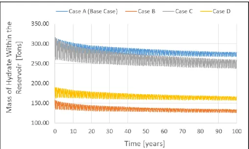
In Figure 10-Figure 14 and Table 3 andTable4, the Base Case results for ±1.5°C/year (section 3.2) were included to facilitate comparison. Figure 10 shows the mass of hydrate within the reservoir for cases A–D. Figure 11 shows the cumulative volumes of gaseous and aqueous CH4 released into the ocean,
for cases A–D, and Figure 12 shows the gaseous and the aqueous CH4 volumetric flow rates across the
19
of gas hydrates within the reservoir. Table 4 summarizes, for cases A–D, the cumulative volumes of aqueous and gaseous CH4 released into the ocean and the time interval in which significant amounts of
gaseous methane were released into the ocean.
Case C (which has higher thermal conductivities in comparison to the Base Case – see Table 1) had the largest reduction in the mass of hydrate within the reservoir (approximately 18% – Figure 10 and Table 3) and the highest volumes of gaseous and aqueous methane released into the ocean (1,270 m3 and
10,314 m3, respectively, Figure 11 and Table 4). For cases A, B and C, significant amounts of gaseous
methane were released into the ocean until approximately 10 years (Figure 11a and Figure 12 and Table 4). After this period, only negligible amounts of gaseous methane flowed through the seafloor (less than 10 m3/y), disappearing completely after ca. 20 years (Figure 12 (A.1), (B.1), (C.1) and insets, Table
4). For case D, significant fluxes of gaseous methane accross the seafloor last for approximately 5 years, and disappear after ca. 10 years (Figure 12 (D.1) and insets, Table 4). Cases B and D had the lowest cumulative volumes of gaseous and aqueous CH4 released into the ocean: approximately 764 m3 and
4,196 m3 (respectively) for case B, and approximately 74 m3 and 5,029 m3 (respectively) for case D
(Figure 11, Table 4). It is worth noting that, although gaseous methane was released into the ocean only in the first years of the simulations, aqueous methane release, in turn, persisted over the 100 years simulated, for all the cases (A–D) (Figure 11 and Figure 12).
Case Initial mass of hydrates within the reservoir [tons]
Mass of hydrates within the reservoir after 100 years [tons]
Mass variation A 315.90 278.23 -11.9 % B 157.95 133.57 -15.4 % C 315.90 259.24 -17.9 % D 189.59 166.41 -12.2 %
Table 3 – Initial and final mass of hydrates, and mass variation, within the reservoir, for cases A–D, for a seasonal BWT oscillation of ±1.5°C/year, after 100 years.
20
Case
Cumulative volume of aqueous CH4 released into the ocean [m3]
Cumulative volume of gaseous CH4 released
into the ocean [m3]
Approximate time interval [years] during which significant amounts of gaseous CH4 were released into
the ocean
A 6,771 1,000 10
B 4,196 764 10
C 10,314 1,270 10
D 5,029 74 5
Table 4 – Cumulative volumes of aqueous and gaseous CH4 released to the ocean and the approximate time
interval in which significant amounts of gaseous methane releases into the ocean occurred, for cases A–D with seasonal BWT oscillation of ±1.5°C/year, over 100 years.
Figure 10 – Mass of hydrate within the reservoir for cases A–D, for a seasonal BWT oscillation of ±1.5°C/year, over 100 years.
21 Figure 11 – Cases A–D, (a) Cumulative volume of gaseous CH4 released into the ocean, and (b) Cumulative
22 Figure 12 Gaseous (1) and aqueous (2) CH4 volumetric flowrates across the seafloor for the Base Case (A.1 and
A.2), for case B (B.1 and B.2), for case C (C.1 and C.2) and for case D (D.1 and D.2), for a seasonal BWT oscillation of ±1.5°C/year, over 100 years.
Figure 13 shows the gas hydrate saturations at t = 0 (initial state), 25, 50 and 100 years, for cases A–D, for a seasonal BWT oscillation of ±1.5°C/year, and Figure 14 shows the gas saturations for cases A–D, at t = 100 years, for the ±1.5°C/year oscillation. For all the cases, the MHSZ changed according to the seasonal BWT oscillation. After 100 years, the MHSZ receded downslope for all the cases (Figure 13
)
.23
The low values of gas saturations in the models after 100 years (Figure 14) are due to hydrate formation owing to cooling BWT, at the end of the simulations.
Figure 13 – Cases A–D, gas hydrate saturations (SH) at 0.00, 25, 50 and 100 years, for a seasonal BWT
24 Figure 14 – Cases A–D, gas saturations (SG), at t = 100 years of a seasonal BWT oscillation of ±1.5°C/year.
4. DISCUSSION
Several previous numerical studies have been carried out to understand how gas hydrates may be related to gas release from the seafloor to the water column and potentially to the atmosphere, over timescales of tens to hundreds of years (e.g. Reagan and Moridis, 2008; Reagan et al., 2009; Thatcher et al., 2013; Marín-Moreno et al., 2013, 2015a, 2015b; Stranne et al., 2016a, 2016b, 2017). However, only two of them (Thatcher et al., 2013 and Marín-Moreno et al., 2015a) investigated the effect of seasonal BWT
25
oscillations on the methane hydrate stability zone (MHSZ). Berndt et al. (2014) used field data and a numerical model applied to an area of seepage at the upper limit of the MHSZ off Svalbard, to conclude that seasonal BWT fluctuations may cause periodic gas hydrate formation and dissociation. The authors suggested the existence of both a permanent and a seasonal MHSZ in the studied area, the latter extending beyond the edge of the permanent stability zone.
Our results indicate that, as suggested by Berndt et al. (2014) for Svalbard, the Rio Grande Cone also presents both a permanent and a seasonal MHSZ along its upper limit in Area E (Figure 15). This division of the MHSZ probably exists in any system with similar topography and temperature oscillations. Due to the low inclination (1.5°) and relatively small horizontal extension (1 km), the seasonal zone extends downslope rapidly to the edge of the model and beyond. Within this zone, our model shows alternate hydrate formation and dissociation, during periods of cooling and warming BWTs, respectively. As this process occurs during the 100-year simulations, the seasonal region increases both in the horizontal (ΔX) and in the vertical (ΔZ) directions (Figure 15), while the permanent zone decreases, with its wedge left tip shrinking downslope, and its upper boundary moving downwards, away from the seafloor (Figure 13). Our results indicate that these horizontal and vertical variations in the seasonal MHSZ (ΔX and ΔZ, respectively, in Figure 15), depends on (1) the seasonal BWT oscillation amplitude, (2) on the sediment properties (porosity, thermal conductivities) and initial hydrate saturation, and (3) on the time in which the system is exposed to the BWT oscillation. In approximately 10 years (for the Base Case), the alternate formation-dissociation cycles reach a moment in which part of the gas released during the hydrate dissociation process (warming stages) is unable to reach the top of the model, and it is trapped again as hydrate in the cooling stages. As a result, significant amounts of gaseous CH4 are released into the ocean only up to 10 years. The other part of the gas
released from hydrate dissociation during the warming stages dissolves in the aqueous phase, and aqueous methane escapes to the ocean over the 100 years simulated.
26 Figure 15 - Schematic representation of the permanent and seasonal MHSZ.
Miller et al. (2015) state that the relatively continuous bottom-simulating reflector (BSR) in the area of the Rio Grande Cone represents the boundary between gas hydrate at the base of the MHSZ and free gas accumulations beneath. The authors also discuss the presence of faults and chimneys in the Rio Grande Cone, stating that they are apparently the main conduits for the methane that forms hydrates near the seafloor, which means that gas may be migrating upward within the sediments from deeper regions, which may explain the existence of seepage features in the studied area too (Ketzer et al., 2019). Our current models do not account for either free gas below the MHSZ, nor for faults or chimneys, and did not include a methane generation or flow from deeper regions. These features would influence significantly the results, especially the amount and the time intervals of methane releases into the ocean: with fluxes and pathways facilitating migration upward within the sediments, more gaseous CH4 could reach the seafloor and escape to the ocean. In addition, the time intervals in which significant
amounts of gaseous CH4 were released into the ocean would be greater than the 10 years indicated by
our results. Without considering these features, and constrained to the limitations of the models, our results indicate that hydrate dissociation itself can release gaseous methane into the ocean due to seasonal BWT oscillations for up to a few decades. Therefore, persistent gas seeps over longer timescales require either a continuing supply of free gas from deeper regions, or a longer-term BTW increase (e.g., contemporary climate change) that continuously changes the MHSZ and destabilizes the hydrate deposits.
27
Due to a lack of information available on the Rio Grande Cone, some of the model’s properties, such as initial hydrate saturation, porosity and thermal conductivities were taken from other published modeling studies and thus, sensitivity tests were carried out to investigate the influence of these parameters. The Base Case was set up with an initial hydrate saturation of 5%. Klauda and Sandler (2005) calculated a global average value of 3.4% for hydrate saturation, different from the common a
priori assumption of 5% for an overall global value. Reagan and Moridis (2008) investigated the effect
of different initial hydrate saturations in 1D methane hydrate-bearing systems, exposed to different BWT linear increasing scenarios. They found that deposits with higher initial hydrate saturation could result in larger methane releases at the seafloor. Our results indicate that, for seasonal BWT oscillations scenarios, initial hydrate saturation also plays an important role in the volume of gas released into the ocean and in the time interval in which this release occurs. The case with initial hydrate saturation of 3% showed the smallest volume of gaseous methane released into the ocean and the smallest time interval during which significant amounts of gaseous methane were released into the ocean (approximately 5 years). Considering that the area E pockmark field has an estimated area of roughly 38 km2 (Ketzer et al., 2019), the average annual release (up to 5 years) was calculated between 0.56
million m3/year (Case D) and 4.82 million m3/year (Case C) of methane. Field data are not yet available
for comparison.
Another important parameter is thermal conductivity. Reagan and Moridis (2008) and Reagan et al. (2009) used 3.3 W.m-1.K-1 and 1.0 W.m-1.K-1 for wet and dry thermal conductivities, respectively.
However, in other modeling studies, authors used lower values: 1.0-1.5 W.m-1.K-1 (approximately) for
wet thermal conductivity and 0.34 W.m-1.K-1 and 0.55 W.m-1.K-1 for dry thermal conductivity
(Marín-Moreno et al., 2013, 2015a, 2015b; Stranne et al., 2016a, 2016b, 2017). Our results indicate that, for seasonal BWT oscillations scenarios, thermal conductivities play an important role in the volumes of gaseous and aqueous methane released into the ocean, since the case with higher thermal conductivities (the same values used by Reagan and Moridis, 2008 and Reagan et al., 2009), showed the largest volumes of CH4 released into the ocean, as a larger region of the stability zone is reached by the
temperature oscillations. However, our results indicate that thermal conductivities do not affect significantly the time interval during which the gaseous methane release into the ocean occurs, since
28
the case with higher thermal conductivities showed the same time interval of significant gaseous methane release into the ocean as the other cases with the same initial hydrate saturation (approximately 10 years). Porosity changes are directly linked to conductivity. A decrease in porosity (Case B vs. Case A) has a similar effect as increasing conductivity (Case C vs. Case A), as the contribution of rock conductivity for heat transfer is higher. In both situations, the amount of hydrate dissociation is higher than in the Base Case, as observed in Table 3 – reduction in mass hydrate goes from -11.9% to -15.4% when porosity is reduced to 30%, and to -17.9% when conductivity is increased to 3.3 W.m-1.K-1. This
relationship was already indicated by Stranne et al (2016).
5. CONCLUSIONS
In this study, we used numerical simulations to investigate how seasonal BWT oscillations affect the methane hydrate stability zone, as well as how much gaseous and aqueous methane is released into the ocean over a timescale of 100 years. TOUGH+HYDRATE was used to model a 2D section across the upper limit of the MHSZ on the Rio Grande Cone, Pelotas Basin, offshore southern Brazil. We defined a Base Case – case A, and three sensitivity tests – cases B, C and D, in which we used lower porosity, higher thermal conductivities and lower initial hydrate saturation, respectively. For the Base Case, we also ran a simulation with a seasonal BWT oscillation of ±0.5°C/year, over 100 years, in order to compare to the results of ±1.5°C/year. We also presented results for a single seasonal BWT oscillation cycle (i.e., 1-year period), for the Base Case, for ±1.5°C/year and ±0.5°C/year. Since we did not consider either free gas in the system during initialization, nor methane generation or upward flow from deeper regions, we could investigate how much methane was released into the ocean due to hydrate dissociation alone, triggered by the seasonal temperature variations. Simulations that include methane recharge scenarios in the models are currently under way.
The results indicate that:
The MHSZ varied periodically due to the seasonal BWT oscillations and receded downslope
29
hydrate and gas saturations in the MHSZ, defining a permanent and a seasonal MHSZ. A larger permeant region of the MHSZ remains mostly unaffected.
Significant volumes of gaseous methane were released into the ocean during the first 10 years
On the other hand, aqueous methane was released into the ocean during the 100 years simulated.
Seasonal BWT oscillations alone could not account for long-term (e.g., century scale) gas seeps
from the MHSZ upper limit. A continuous supply of free gas from deeper regions, or a constant temperature increase due to, for instance, global climate change or natural variations, would be necessary to explain the observed seeps.
With regard to the sensitivity tests, the results indicate that:
For a lower porosity (case B; porosity = 30%), the volumes and the fluxes of gaseous and
aqueous methane released into the ocean were smaller than those for the Base Case (porosity = 60%) were. The percentage of reduction in hydrate mass, however, is higher when porosity decreases, as the contribution of rock conductivity is higher leading to increased heat flow.
For higher thermal conductivities (case C; 3.3 W.m-1.K-1) related to the Base Case (1.21 W.m -1.K-1), the volumes and the fluxes of gaseous and aqueous methane released into the ocean were
the largest of all the cases studied. This indicates that thermal conductivities play an important role in methane release into the ocean, for seasonal BWT oscillation scenarios.
For a lower initial hydrate saturation (case D; 3%) relative to the other cases (5%), the volume
and the flux of gaseous methane released into the ocean were the smallest of all the cases studied. Significant gaseous methane flows into the ocean, for case D, occurred up to 5 years, unlike cases A, B and C, for which gaseous methane flows into the ocean occurred up to 10 years (for a BWT oscillation of ±1.5°C/year, over 100 years). This indicates that initial hydrate
30
saturation is an important parameter for seasonal BWT oscillation scenarios, since it plays an important role in methane release into the ocean.
ACKNOWLEDGMENTS
This study has been supported by PETROBRAS and financed in part by the Coordenação de Aperfeiçoamento de Pessoal de Nível Superior - Brasil (CAPES), and has been developed in the Institute of Petroleum and Natural Resources – IPR, at Pontifical Catholic University of Rio Grande do Sul – PUCRS, Porto Alegre, Brazil. Daniel Praeg was supported through funding from the European Union’s Horizon 2020 research and innovation program under Marie Skłodowska-Curie grant agreement No. 656821.
REFERENCES
Berndt, C., Feseker, T., Treude, T., Krastel, S., Liebetrau, V., Niemann, H., Bertics, V.J., Dumke, I., Dünnbier, K., Ferré, B., Graves, C., Gross, F., Hissmann, K., Hühnerbach, V., Krause, S., Lieser, K., Schauer, J., Steinle, L., 2014. Temporal Constraints on Hydrate-Controlled Methane Seepage off Svalbard. Science (80-. ). 343, 284 LP – 287. https://doi.org/10.1126/science.1246298
Kretschmer, K., Biastoch, A., Rüepke, L., Burwicz, E., 2015. Modeling the fate of methane hydrates under global warming. Global Biogeochem. Cycles 29. https://doi.org/10.1002/2014GB005011 Collett, T.S., Johnson, A.H., Knapp, C.C., Boswell, R., 2009. Natural Gas Hydrates: A Review. Nat.
Gas Hydrates—Energy Resour. Potential Assoc. Geol. Hazards.
https://doi.org/10.1306/13201142M891602
Dillon, William P. Discussion of the Paper “Hydrates Offshore Brazil”. Annals of the New York Academy of Sciences vol. 715, 114-118. 1994.
Floodgate, G.D., Judd, A., 1992. The origins of shallow gas. Cont. Shelf Res. 12, 1145–1156. https://doi.org/10.1016/0278-4343(92)90075-U
Fontana, R.L., Mussumeci, A.. Hydrates offshore Brazil. Annals of the New York Academy of Sciences, vol. 715, 106-113, 1994.
Hester, Keith C.; Brewer, Peter G. Clathrate Hydrates in Nature. Annual Review of Marine Science, vol. 1, 303-327, 2009. doi: 10.1146/annurev.marine.010908.163824.
Ketzer, M., Praeg, D., Pivel, M.A.G., Augustin, A.H., Rodrigues, L.F., Viana, A.R., Cupertino, J.A., 2019. Gas Seeps at the Edge of the Gas Hydrate Stability Zone on Brazil’s Continental Margin. Geosciences 9, 193. https://doi.org/10.3390/geosciences9050193
Klauda Jeffrey B.; Sandler Stanley I. Global Distribution of Methane Hydrate in Ocean Sediment. Energy and Fuels, vol. 19, 459-470, 2005. doi: 10.1021/ef049798o.
Kvenvolden, K.A., 1993. Gas hydrates—geological perspective and global change. Rev. Geophys. 31, 173–187. https://doi.org/10.1029/93RG00268
31
Locarnini, R. A., A. V. Mishonov, J. I. Antonov, T. P. Boyer, H. E. Garcia, O. K. Baranova, M. M. Zweng, and D. R. Johnson, 2010. World Ocean Atlas 2009, Volume 1: Temperature. S. Levitus, Ed. NOAA Atlas NESDIS 68, U.S. Government Printing Office, Washington, D.C., 184 pp.
Marín-Moreno H., Minshull T. A., Westbrook G. K., Sinha B., Sarkar S. The response of methane
hydrate beneath the seabed offshore Svalbard to ocean warming during the next three centuries.
Geophysical Research Letters, vol. 40, 5159-5163, 2013. doi:10.1002/grl.50985.
Marín-Moreno H., Minshull T. A., Westbrook G. K., Sinha B. Estimates of future warming-induced
methane emissions from hydrate offshore west Svalbard for a range of climate models. Geochem.
Geophys. Geosyst., 16, 1307–1323, 2015a. doi:10.1002/2015GC005737.
Marín-Moreno H., Giustiniani M., Tinivella U. The potential response of the hydrate reservoir in the
South Shetland Margin, Antarctic Peninsula, to ocean warming over the 21st century. Polar Research, 34:1, 27443, 2015b. doi: 10.3402/polar.v34.27443.
Mienert, J., Vanneste, M., Bünz, S., Andreassen, K., Haflidason, H., Petter Sejrup, H., 2005. Ocean warming and gas hydrate stability on the Mid-Norwegian Margin at the Storegga Slide. Mar. Pet. Geol. 22, 233–244. https://doi.org/10.1016/j.marpetgeo.2004.10.018
Miller, J.D., Ketzer, J. M., Viana, A. R., Kowsmann, R. O., Freire, A .F. M., Oreiro, S. G., Augustin, A. H., Lourega, R. V., Rodrigues, L. F., Heemann, R., Preissler, A. G., Machado, and C. X, Sbrissa, G. F. Natural gas hydrates in the Rio Grande Cone (Brazil): A new province in the western South Atlantic, Marine and Petroleum Geology 67 (2015) 187-196, 2015. doi.org/10.1016/j.marpetgeo.2015.05.012. Moridis G. J., Kowalsky M. B., and Pruess, K. TOUGH+HYDRATE v1.2 User’s Manual: A code for
the Simulation of System Behavior in Hydrate-Bearing Geologic Media, Lawrence Berkeley National
Laboratory, Berkeley, Calif., 2012.
Reagan, M. T., Moridis, J. G. Dynamic response of oceanic hydrate deposits to ocean temperature
change, J. Geophys Res., 113, C12023, 2008. doi:10.1029/2008JC004938.
Reagan, M. T., Moridis, J. G., Zhang, K. Large-scale simulation of oceanic gas hydrate dissociation in
response to climate change, Lawrence Berkeley National Laboratory, Berkeley, Calif., 2009.
Serov, P., Vadakkepuliyambatta, S., Mienert, J., Patton, H., Portnov, A., Silyakova, A., Panieri, G., Carroll, M.L., Carroll, J., Andreassen, K., Hubbard, A., 2017. Postglacial response of Arctic Ocean gas hydrates to climatic amelioration. Proc. Natl. Acad. Sci. 114, 6215 LP – 6220. https://doi.org/10.1073/pnas.1619288114
Stranne C., O´Reagan M., Jakobsson. Overestimating climate warming-induced methane gas escape
from the seafloor by neglecting multiphase flow dynamics, Geophys. Res. Lett., 43, 8703–8712, 2016a.
doi:10.1002/2016GL070049.
Stranne C., O´Reagan M., Dickens G. R., Crill P., Miller C., Preto P., Jakobsson M. Dynamic
simulations of potential methane release from East Siberian continental slope sediments. Geochem.
Geophys. Geosyst., 17, 2016b. doi:10.1002/2015GC006119,.
Stranne, C.; O’Reagan, M. Conductive heat flow and nonlinear geothermal gradients in marine
sediments—observations from Ocean Drilling Program boreholes. Geo-Marine Lett., 36, 2016a, 25–
33.
Stranne C., O´Reagan M., Jakobsson. Modeling fracture propagation and seafloor gas release during
seafloor warming-induced hydrate dissociation, Geophys. Res. Lett., 44, 8510–8519, 2017.
32
Thatcher K. E.; Westbrook G. K.; Sarkar S.; Minshull T. A. Methane release from warming-induced
hydrate dissociation in the West Svalbard continental margin: Timing, rates, and geological controls.
J. Geophys. Res. Solid Earth, vol. 118, 22-38, 2013. doi:10.1029/2012JB009605.
Tréhu, Anne M.; Ruppel, Carolyn; Holland, Melanie; Dickens, Gerald R.; Torres, Marta E.; Collet, Timothy S.; Goldberg, David; Riedel, Michael; Schultheiss, Peter. Gas Hydrates in Marine Sediments.
Lessons from Scientific Ocean Drilling. Oceanography, vol. 19, No. 4, 2006. doi.org/10.5670/oceanog.2006.11.
Westbrook, G.K., Thatcher, K.E., Rohling, E.J., Piotrowski, A.M., Pälike, H., Osborne, A.H., Nisbet, E.G., Minshull, T.A., Lanoisellé, M., James, R.H., Hühnerbach, V., Green, D., Fisher, R.E., Crocker, A.J., Chabert, A., Bolton, C., Beszczynska-Möller, A., Berndt, C., Aquilina, A., 2009. Escape of methane gas from the seabed along the West Spitsbergen continental margin. Geophys. Res. Lett. 36. https://doi.org/10.1029/2009GL039191