Techniques for asteroid spectrocopy

HAL Id: tel-00785991

https://tel.archives-ouvertes.fr/tel-00785991

Submitted on 7 Feb 2013

HAL is a multi-disciplinary open access archive for the deposit and dissemination of sci-entific research documents, whether they are pub-lished or not. The documents may come from teaching and research institutions in France or abroad, or from public or private research centers.

L’archive ouverte pluridisciplinaire HAL, est destinée au dépôt et à la diffusion de documents scientifiques de niveau recherche, publiés ou non, émanant des établissements d’enseignement et de recherche français ou étrangers, des laboratoires publics ou privés.

Techniques for asteroid spectrocopy

Marcel Popescu

To cite this version:

Marcel Popescu. Techniques for asteroid spectrocopy. Earth and Planetary Astrophysics [astro-ph.EP]. Observatoire de Paris; Universitatea Politehnica din Bucuresti, Facultatea de Ştiinţe Aplicate, 2012. English. �tel-00785991�

ÉCOLE DOCTORALE D’ASTRONOMIE ET D’ASTROPHYSIQUE

D’ÎLE-DE-FRANCE

∗

UNIVERSITATEA POLITHENICA BUCURE ¸STI

FACULTATEA DE ¸STIIN ¸

TE APLICATE

DOCTORAL THESIS

by

Marcel Popescu

TECHNIQUES FOR ASTEROID SPECTROSCOPY

Defended the 23 Octobre 2012 before the jury:

Vasile IFTODE (Universitatea Polithenica Bucure¸sti) President Olivier GROUSSIN (Laboratoire d’Astrophysique de Marseille) Reviewer Petre POPESCU (Institutul Astronomic al Academiei Române) Reviewer

Dan DUMITRA ¸S (INFLPR, România) Reviewer

Jean SOUCHAY (SYRTE - Observatoire de Paris) Examiner Mirel BIRLAN (IMCCE - Observatoire de Paris) Co-Advisor Constantin P. CRISTESCU (Universitatea Polithenica, Bucure¸sti) Co-Advisor

ÉCOLE DOCTORALE D’ASTRONOMIE ET D’ASTROPHYSIQUE

D’ÎLE-DE-FRANCE

∗

UNIVERSITATEA POLITHENICA BUCURE ¸STI

FACULTATEA DE ¸STIIN ¸

TE APLICATE

THÈSE DE DOCTORAT

par

Marcel Popescu

TECHNIQUES D’OBSERVATION SPECTROSCOPIQUE D’ASTÉROÏDES

Soutenue le 23 Octobre 2012 devant un jury composé de :

Vasile IFTODE (Universitatea Polithenica, Bucure¸sti) Présidente Olivier GROUSSIN (Laboratoire d’Astrophysique de Marseille) Rapporteur Petre POPESCU (Institutul Astronomic al Academiei Române) Rapporteur

Dan DUMITRA ¸S (INFLPR, România) Rapporteur

Jean SOUCHAY (SYRTE - Observatoire de Paris) Examinateur

Mirel BIRLAN (IMCCE - Observatoire de Paris) Co-Directeur de thèse Constantin P. CRISTESCU (Universitatea Polithenica, Bucure¸sti) Co-Directeur de thèse

ÉCOLE DOCTORALE D’ASTRONOMIE ET D’ASTROPHYSIQUE

D’ÎLE-DE-FRANCE

∗

UNIVERSITATEA POLITHENICA BUCURE ¸STI

FACULTATEA DE ¸STIIN ¸

TE APLICATE

TEZ ˘

A DOCTORAT

autor

Marcel Popescu

TEHNICI DE OBSERVA¸

TIE SPECTROSCOPIC ˘

A PENTRU ASTEROIZI

Sus¸tinut˘a în 23 Octombrie 2012 în fa¸ta juriului:

Vasile IFTODE (Universitatea Polithenica Bucure¸sti) President Olivier GROUSSIN (Laboratoire d’Astrophysique de Marseille) Reviewer Petre POPESCU (Institutul Astronomic al Academiei Române) Reviewer

Dan DUMITRA ¸S (INFLPR, România) Reviewer

Jean SOUCHAY (SYRTE - Observatoire de Paris) Examiner Mirel BIRLAN (IMCCE - Observatoire de Paris) Co-Advisor Constantin P. CRISTESCU (Universitatea Polithenica, Bucure¸sti) Co-Advisor

evolution of the Solar System. For achieving this goal, the asteroids are of a special interest to the astronomical community as a possible window back to the beginning of the planetary for-mation. Being the only remnants of the early stages of planetary history they recorded the com-plex chemical and physical evolution that occurred in the solar nebula. Thus, the knowledge of both dynamical and physical properties of the current asteroid population brings valuable information for understanding the Solar System and more generally other planetary systems.

In this thesis I present the project Modeling for Asteroids (acronym M4AST). M4AST is an on-line service that I developed for modeling surfaces of asteroids using several theoretical approaches. M4AST consists into a database containing more than 2,500 spectra of asteroids together with a library of routines which can model and extract several mineralogical param-eters. The database M4AST could be accessed via its own webpage interface as well as via the Virtual Observatory (VO-Paris) protocols. This service is available to the web address http://cardamine.imcce.fr/m4ast. It allows several routines for modeling spectra: taxonomic classification, space weathering effects modeling, comparison to laboratory spectra of mete-orites and minerals, band centers and band area computing.

I have participated to more than 10 observational campaigns for observing both physical and orbital parameters of asteroids. The objective of spectral runs was to characterize the mineralogical properties of these bodies based on their reflectance spectra. Astrometry was mainly devoted to the confirmation and secures orbits of new discovered asteroid.

During the thesis I observed and characterized near-infrared spectra of eight Near Earth Asteroids namely 1917, 8567, 16960, 164400, 188452, 2010 TD54, 5620, and 2001 SG286. These observations were obtained using the NASA telescope IRTF equipped with the spectro-imager SpeX, and the CODAM-Paris observatory facilities. Based on these spectra mineralog-ical solutions were proposed for each asteroid. The taxonomic classification of five of these objects was reviewed and a corresponding type was assigned to the other three asteroids that were not classified before. Four of the observed objects have delta - V lower than 7 km/sec, which make them suitable targets in terms of propulsion for a future spacecraft mission. The asteroid (5620) Jasonwheeler exhibits spectral behaviors similar to the carbonaceous chondrite meteorites.

I observed and modeled six Main Belt Asteroids. (9147) Kourakuen, (854) Frostia, (10484) Hecht and (31569) 1999 FL18 show the characteristics of V-type objects, while (1333) Cevenola, (3623) Chaplin belong to S-complex. Some of them have some peculiar properties: (854) Fros-tia is a binary asteroid, (10484) Hecht and (31569) 1999 FL18 have pairs, (1333) Cevenola, (3623) Chaplin show large amplitude lightcurves. The taxonomic classification, the compar-isons to the meteorite spectra from the Relab database and the mineralogical analysis converged to the same solutions for each of these objects, allowing to find important details for the chem-ical compositions and resemblances to the Howardite-Eucrite-Diogenite class of meteorites.

tion et de l’évolution du Système Solaire. Pour atteindre cet objectif les astéroïdes présentent un intérêt tout particulier pour la communauté scientifique. En effet, nous pouvons regarder la population astéroïdale comme une fenêtre vers le passée, par laquelle nous regardons les débuts de la formation du système planétaire. Ils sont les témoins des premiers moments de la formation des planètes gardant dans leur structure la complexité chimique de la nébuleuse primordiale. Pour cette raison, les études physiques et dynamiques de ces corps nous appor-tent des informations essentielles sur l’histoire et l’évolution de notre Système Solaire et plus généralement sur la formation des systèmes planétaires.

Pendant ma thèse j’ai développé l’application Modelling for Asteroids (acronyme M4AST). M4AST est un service en libre service sur internet permettant la modélisation des surfaces d’astéroïdes en utilisant plusieurs approches théoriques. M4AST est composé d’une base de données contenant quelques 2500 spectres d’astéroïdes et d’une bibliothèque de routines permettant la modélisation et l’obtention de plusieurs paramètres minéralogiques. La base de données est accessible aussi bien par les biais des protocoles de l’Observatoire Virtuel (OV-Paris) que par sa propre interface. Le service est accessible depuis l’adressehttp://

cardamine.imcce.fr/m4ast. M4AST permet plusieurs types d’analyses :

classifi-cation taxonomique, modélisation de l’altération spatiale, comparaison avec les spectres des météorites et des minéraux terrestres, calculs des centres et des surfaces des bandes.

J’ai participé à plus de 10 campagnes d’observations pour la caractérisation physique et dynamique des astéroïdes. Les observations spectroscopiques ont servi à la caractérisation minéralogique des surfaces d’astéroïdes. L’astrométrie a plutôt servi à la confirmation et la sécurisation de nouvelles découvertes d’astéroïdes. Pendant la thèse, j’ai observé et carac-térisé les spectres en infrarouge proche de huit astéroïdes géocroiseurs : 1917, 8567, 16960, 164400, 188452, 2010 TD54, 5620, and 2001 SG286. Ces observations ont été obtenues avec le télescope IRTF et du spectrographe SpeX, en employant l’infrastructure CODAM de l’Observatoire de Paris. Pour chaque astéroïde j’ai proposé des solutions minéralogiques. Une révision de leur taxonomie a aussi été effectuée pour cinq astéroïdes de mon échantillon. Qua-tre des objets sont des objets à faible delta-V, qui sont des cibles souhaitables/possibles pour des missions spatiales. L’astéroïde (5620) Jasonwheeler montre un spectre similaire à ceux des météorites chondritiques.

J’ai observé et modélisé six astéroïdes de la ceinture principale. (9147) Kourakuen, (854) Frostia, (10484) Hecht and (31569) 1999 FL18 montrent des caractéristiques des astéroïdes du type V; (1333) Cevenola, (3623) Chaplin sont du type taxonomique S. Quelques astéroïdes de cet échantillon sont particuliers : (854) Frostia est un astéroïde binaire, (10484) Hecht et (31569) 1999 FL18 ont des gémeaux dynamiques, (1333) Cevenola et (3623) Chaplin sont des objets avec des courbes de lumières à grandes amplitudes. La classification taxonomique, la comparaison avec les météorites, permettent l’établissement des solutions minéralogiques

intéressantes et des ressemblances avec les météorites de la classe des howardites, eucrites et diogenites.

Sistemului Solar. În atingerea acestui obiectiv asteroizii prezint˘a un interes special pentru co-munitatea ¸stiin¸tific˘a. Popula¸tia de asteroizi poate fi privit˘a ca o fereastr˘a spre trecut, prin care se pot cunoa¸ste originile Sistemului Solar. Astfel, asteroizii sunt m˘arturiile primelor momente ale form˘arii planetelor, p˘astrând în structura lor complexitatea chimic˘a a nebuloasei primor-diale. Din acest motiv, studiile fizice ¸si dinamice ale acestor corpuri aduc informa¸tii esen¸tiale despre istoria ¸si evolu¸tia sistemului nostru solar ¸si generalizând despre formarea altor sisteme planetare.

Pentru realizarea acestei teze am dezvoltat aplica¸tia Modelling for Asteroids (M4AST). M4AST este un serviciu gratuit, care poate fi accesat online. Acesta permite modelarea propri-et˘a¸tilor fizice ale suprafe¸telor de asteroizi utilizând mai multe abord˘ari teoretice. M4AST este compus dintr-o baz˘a de date care con¸tine peste 2 500 de spectre de asteroizi ¸si un set de ru-tine care permit modelarea ¸si ob¸ru-tinerea mai multor parametrii mineralogici. Baza de date este accesibil˘a ¸si indirect folosind protocolul Observatorului Virtual (OV - Paris). Serviciul este accesibil la adresahttp://cardamine.imcce.fr/m4ast. M4AST permite mai multe tipuri de analize: clasificarea taxonomic˘a, modelarea alter˘arii spa¸tiale, compara¸tia spectral˘a cu meteori¸tii ¸si mineralele terestre, calculele centrelor de band˘a ¸si ariilor benzilor.

Am participat la mai mult de 10 campanii de observa¸tii pentru caracterizarea fizic˘a ¸si di-namic˘a a asteroizilor. Observa¸tiile spectroscopice au servit la caracterizarea mineralogic˘a a suprafe¸telor asteroizilor. În perioada tezei am ob¸tinut ¸si analizat spectrele în infraro¸su a opt asteroizi geointersectori (asteroizi ce se apropie sau intersecteaz˘a orbita P˘amântului): 1917, 8567, 16960, 164400, 188452, 2010 TD54, 5620 ¸si 2001 SG286. Aceste observa¸tii au fost ob¸tinute cu ajutorul telescopului IRTF ¸si al spectografului SpeX, utilizând infrastructura CO-DAM a Observatorului din Paris. Pentru fiecare asteroid am propus solu¸tii mineralogice. O revizuire a taxonomiei lor a fost efectuat˘a pentru cinci astroizi din acest e¸santion. Patru din-tre obiecte sunt obiecte cu delta - V mic, acestea fiind ¸tinte posibile pentru misiunile spa¸tiale. Asteroidul (5620) Jasonwheelr prezint˘a un spectru similar cu cel al meteori¸t ilor condritici.

Am observat ¸si modelat spectrele a ¸sase asteroizi din centura principal˘a. (9147) Kourakuen, (854) Frostia, (10484) Hecht ¸si (31569) 1999 FL18 prezint˘a caracteristici ale asteroizilor de tipul V. (1333) Cevenola, (3623) Chaplin sunt de tipul taxonomic S. Aceste ¸sase obiecte au câteva propriet˘a¸ti remarcabile: (854) Frostia este un asteroid binar, (10484) Hecht ¸si (31569) 1999 FL18 au perechi dinamice, (1333) Cevenola ¸si (3623) Chaplin sunt obiecte care au curbe de lumin˘a cu amplitudini mari. Clasificarea taxonomic˘a, compara¸tia cu meteori¸tii, permit sta-bilirea de solu¸tii mineralogice interesante.

Foremost, I would like to express my sincere gratitude to my advisors Mirel Birlan and Constantin P. Cristescu for their continuous support of my Ph.D study and research, for their patience, motivation, enthusiasm, and immense knowledge. I am grateful to Mirel also for the observational data, the telescope time and the scholarships. He also took care of all the administrative staff and ensured me with a very pleasant stay in Paris (thanks also to Mariana, Mirela, Daniel and Florian).

I would like to thank my thesis committee: Vasile Iftode - the jury president, Olivier Groussin, Petre Popescu, Dan Dumitra¸s - the reviewers, and Jean Souchay the examiner, for evaluating my work, and for their constructive and helpful suggestions.

I am grateful to the colleagues from IMCCE - Observatoire de Paris, for the chance to visit and to be a part of the institute. Thank you for welcoming me as a friend and helping to develop the ideas in this thesis.

I thank to Dan Alin Nedelcu for the encouragement, for insightful comments, and for all the help during the period I wrote my thesis at Astronomical Institute of Romanian Academy. I am also grateful for getting me in your team at AIRA.

I thank to Ovidiu Vaduvescu for the opportunity to become astronomer. Our collaborations were very fruitful for me, and I will always appreciate the help you gave me at the beginning of my career.

I also want to thank to all of my friends from Admiral V. Urseanu Observatory and from Astroclubul Bucure¸sti. In particular, I want to thank to Adrian ¸Sonka, Oana Sandu, Radu Gherase and Marian Naiman for all the evenings full of astronomy, for all the discussions we had and for all star parties.

Last but not the least, I would like to thank my future wife - Andreea, for her love and support over the past two years. To my Mom and Dad, to my brother Bogdan, and to my aunt Silvia, I am grateful for their support and encouragement.

Tables 22

Figures 27

I INTRODUCTION 29

1 Why asteroids? 31

1.1 The place of asteroids in the structure of the Solar System . . . 31

1.2 The Discovery Of Asteroids . . . 33

1.3 Distribution and diversity of asteroids . . . 35

1.4 Asteroid brightness and albedo . . . 38

1.5 My contribution to asteroids discovery . . . 38

2 Why spectroscopy? 43 2.1 Diffraction gratings and prisms . . . 44

2.2 Spectroscopy and atmospheric transparency . . . 46

2.3 A simple application . . . 47

2.4 Spectroscopy for asteroids . . . 50

2.4.1 Reflectance versus emission . . . 50

2.4.2 Spectral features . . . 52

II TECHNIQUES FOR ASTEROID SPECTROSCOPY 55 3 Observing techniques 57 3.1 IRTF Telescope and the SpeX instrument . . . 57

3.2 Planning the observations . . . 58

3.3 Data reduction procedures . . . 59

4 Spectral analysis techniques 65 4.1 Interpretation . . . 65

4.1.1 Taxonomy . . . 65

4.1.2 Spectral comparison - Comparative planetology . . . 68

4.1.3 Space weathering effects . . . 70

4.1.4 Band parameters . . . 71

4.2 Algorithms . . . 72

4.2.1 Taxonomic classification . . . 72

4.2.3 Computing the space weathering effects . . . 74

4.2.4 Application of the Cloutis model . . . 75

5 M4AST - Modeling of Asteroids Spectra 77 5.1 Spectral database . . . 78

5.1.1 Structure of M4AST database . . . 78

5.1.2 The content . . . 79

5.1.3 M4AST database via the Virtual Observatory . . . 80

5.2 The interface . . . 81

5.2.1 Database interface . . . 81

5.2.2 Modeling tool interface . . . 82

5.2.3 Updating the database . . . 84

5.3 Testing of M4AST . . . 84

5.3.1 Results . . . 85

5.3.2 Discussions regarding misinterpretations of spectra . . . 88

III OBSERVATIONS AND RESULTS 91 6 Spectral properties of near-Earth asteroids 93 6.1 Log of observations . . . 94

6.2 S-type Near-Earth Asteroids . . . 95

6.2.1 (1917) Cuyo . . . 96 6.2.2 (8567) 1996 HW1 . . . 97 6.2.3 (16960) 1998 QS52 . . . 100 6.2.4 (188452) 2004 HE62 . . . 101 6.2.5 2010 TD54 . . . 103 6.2.6 (164400) 2005 GN59 . . . 104

6.3 Spectral properties of two primitive NEAs . . . 105

6.3.1 (5620) Jasonwheeler . . . 106

6.3.2 2001 SG286 . . . 108

6.4 Discussion . . . 109

7 Spectral properties of Main Belt Asteroids 113 7.1 Log of observations . . . 113

7.2 (9147) Kourakuen - a V-type asteroid outside Vesta family . . . 115

7.3 A binary asteroid: (854) Frostia . . . 119

7.4 1333 and 3623 - two asteroids with large amplitude lightcurves . . . 123

7.5 Asteroid pairs: (10484) Hecht, (31569)1999 FL18 . . . 129

IV CONCLUSIONS AND PERSPECTIVES 131

8 Conclusions and perspectives 133

A The GuideDog and the BigDog interfaces 135

B List of publications 137

B.1 First Author . . . 137 B.2 Co-Author . . . 137 B.3 Conferences and Workshops . . . 138

2.1 The emission lines identification in spectrum of PG1634 +706. The line labels, their corresponding laboratory wavelengths, these wavelengths shifted with z=

1.34, and the wavelengths observed in the spectrum are presented. . . 50

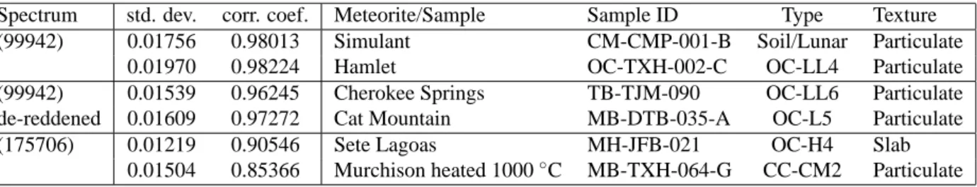
5.1 Summary of the results obtained by matching the asteroids spectra with spec-tra from the Relab database. For each asteroid, I show the best two matches, obtained by measuring the standard deviation (std. dev.) and the correlation coefficient (corr. coef.). . . 85 6.1 Some characteristics of the observed NEAs: orbit type, semi-major axis,

ec-centricity, inclination, absolute magnitude (H), and the delta-V. . . 94 6.2 Log of NEAs observations. Their designations, date of observation with the

fraction of the day for the mid time of the observation, the apparent magnitude, the phase angle, the heliocentric distance, the airmass at the mean UT of each observation, the integration time for each spectrum (ITime), and the number of cycles are shown. . . 95 6.3 The solar analogs used for data reduction in the case of the NEAs spectra. The

airmass at the moment of observations and relative distance to the asteroid are presented. . . 95 6.4 Summary of results obtained by matching the asteroid spectra and de-reddened

asteroid spectra with spectra from the Relab database. The comparison was made using aχ2method and a selection of the obtained results was done based on spectral features (band, band-gap, concavity) positions, and albedo values. For (5620) Jasonwheeler, a de-reddening model was not applied . . . 99 6.5 Slope and Csparameter for the S-type objects studied in this article. The

calcu-lation was made by normalization of spectra to 0.55µm. Objects marked with (*) are normalized to 1.25µm (only for NIR part). . . 110 6.6 Computed parameters from the Cloutis et al. [1986a] model applied to the V+NIR

spectra of (1917) Cuyo, (8567) 1996 HW1, and (16960) 1998 QS52. The esti-mation error for band centers (BI, BII) is_{±0.005. . . 111} 7.1 Some characteristics of our observed MBAs: semi-major axis, eccentricity,

in-clination, absolute magnitude (H), and orbital period. . . 114 7.2 Log of asteroids observations. Asteroid designation, date of observation with

the fraction of the day for the mid time of the observation, apparent magnitude, phase angle, heliocentric distance, the airmass at the mean UT of each observa-tion, the integration time for each spectrum (ITime), and the number of cycles are presented. . . 114

7.3 Solar analogs used for data reduction, their airmass at the moment of observa-tions and their relative distance to the object. . . 115 7.4 Summary of results obtained by matching the main belt asteroids spectra with

spectra from Relab database. The most relevant matches are presented. The comparison coefficients are given together with some details related to the lab-oratory samples. . . 119

1.1 A field obtained with INT-WFC on February 28, 2012. Ten asteroids were iden-tified (marked with pink), from which only three were known at the moment of the observation. The size of the field is (15 arcmin x 15 arcmin) . . . 34 1.2 a) The position of asteroids in the inner part of the Solar System (Source:

http://en.wikipedia.org/). b)The distribution of asteroids in a

rep-resentation (a,e)- bottom and (a,sini) - top, a is the semi-major axis and i the inclination [Nedelcu, 2010]. . . 36 1.3 The flowchart of Mega-Precovery [Vaduvescu et al., 2012]. . . . 39 1.4 The first part of the Minor Planet Electronic Circular issued for the orbit

recov-ery of the asteroid 2007 ES. . . 41 2.1 The diffraction pattern produced by a diffraction grating having b= d = 5µm

and N=1000. Different wavelengths are considered. . . 45 2.2 The atmospheric transmission above Mauna Kea for the wavelength ranges 0.9

- 2.7µm with a water vapor column of 1.6 mm and an air mass of 1 (Source:

http://www.gemini.edu/?q=node/10789). . . 46

2.3 The field of quasar PG1634+706 (north is at bottom of the figure). The object and its spectrum are surrounded by a rectangle. In this image it can be distinguish the zero order (objects are dots) and the first order (light is dispersed)

-Popescu et al. [2012a]. . . . 48 2.4 a) PG1634 + 706 spectrum obtained after data reduction and continuum

sub-traction; b) the correlation coefficient between quasar spectrum and the tem-plate spectrum shifted with different z [Popescu et al., 2012a]. . . . 49 2.5 The components of the radiation received from 1km square lunar mare area

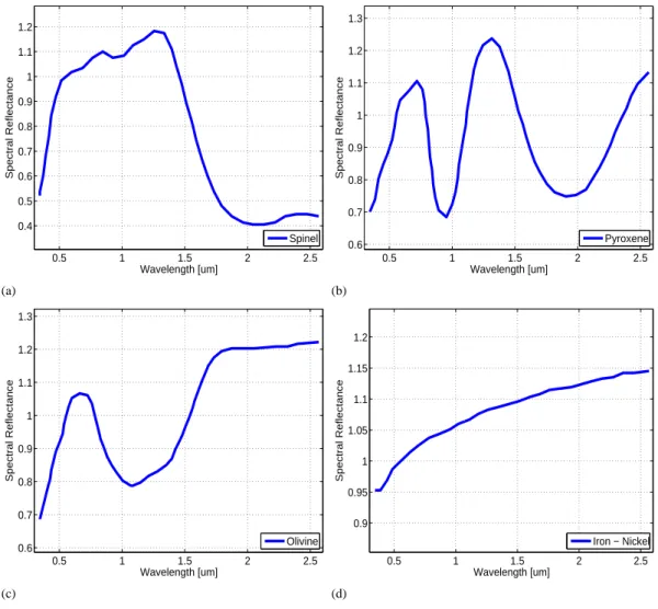
(dark basaltic plain on Moon formed by ancient volcanic eruptions) having an albedo of 006, considering the average Earth-Moon distance, phase angle 0, T = 395K. The flux is measured in Watts per square meter per micron. Source McCord & Adams [1977] . . . 51 2.6 Reflectance spectra of several meteoritic important minerals: a) Spinel, b)

Py-roxene, c) Olivine, d) Iron-Nickel alloy. . . 52 3.1 a) The 3m NASA InfraRed Telescope Facility at the Mauna Kea Observatory

on Hawaii. b) SpeX instrument mounted to IRTF telescope. As scale, SpeX is 1.4m tall and weighs 478kg. . . 58 3.2 The data reduction procedure for NIR spectra obtained with IRTF/SpeX [Nedelcu,

3.3 The raw spectra of an asteroid and standard star. The twos spectra are modu-lated by the absorption bands of the Earth atmosphere (essentially telluric water bands). . . 62

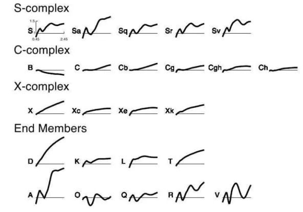
4.1 Bus-DeMeo taxonomy key figures. Source :http://smass.mit.edu/

busdemeoclass.html . . . 68

4.2 a) The photomicrograph of a thin section of the carbonaceous chondrite Al-lende, which was seen to fall in Chihuahua, Mexico on the night of February 8, 1969. Numerous round silicate chondrules together with irregular inclu-sions can been observed . b) Comparison of solar-system abundances (relative to silicon) determined by solar spectroscopy and by analysis of carbonaceous chondrites [Ringwood, 1979]. . . 70 4.3 Different ways in which space weathering affects the visible and near-infrared

spectra of soil. Space weathering processes alters the properties of the soil that covers the surface of all bodies which are not protected by an atmosphere (Sourcehttp://en.wikipedia.org/). . . 71

5.1 M4AST logo and the aims of this project. . . 78 5.2 Block diagram and work flow of M4AST [Popescu et al., 2012b]. . . . 79 5.3 The database interface of M4AST. Here is illustrated the search of a spectrum

for (1917) Cuyo and the result of this search displayed at the bottom of the interface. . . 80 5.4 M4AST web application tool : modelling tool interface . . . 82 5.5 M4AST web tool application: screen-shoot from the table containing the list of

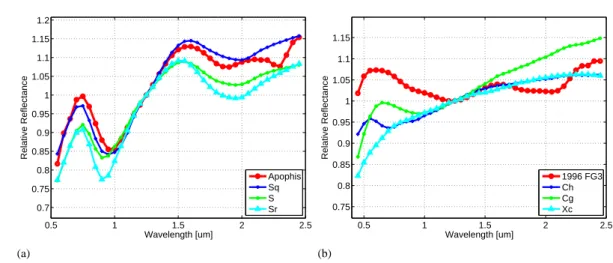
the closest fifty best matches which are ordered upon the comparison coefficient (column two of the table). . . 83 5.6 Classification in Bus-DeMeo taxonomical system for: a)) (99942) Apophis,

and b) (175706) 1996 FG3. All the spectra are normalized to 1.25µm. . . 84 5.7 Classification in the G-mode taxonomical system for: a) (99942) Apophis using

G13 taxonomy, b) (175706) 1996 FG3 using G13 taxonomy, and c) (175706) 1996 FG3 using G9 taxonomy. All the spectra are normalized either to 1.25

oratory spectra:(a) spectrum of Apophis and the spectrum of a simulant Lunar soil, (b) spectrum of Apophis and the spectrum of a particulate sample from the Hamlet meteorite, (c) de-reddened spectrum of Apophis and the spectrum of a particulate sample from the Cherokee Springs meteorite, (d) de-reddened spectrum of Apophis and the spectrum of a particulate sample from the Cat Mountain meteorite, (e) spectrum of 1996 FG3 and the spectrum of a sample from the meteorite Sete Lagoas, and (f) spectrum of 1996 FG3 and the spectrum of a sample from the Murchison meteorite heated to 1000◦C. . . 87

6.1 a) The visible [Binzel et al., 2004b] and the NIR spectrum of (1917) Cuyo; b) a polynomial fit of the V+NIR spectrum of (1917) Cuyo compared with the theoretical spectra of R and Sr types; c) reflectance spectrum of (1917) Cuyo and the closest match resulting from meteorite comparison - H3-4 ordinary chondrite Dhajala; d) De-reddened spectrum of (1917) Cuyo and the closest match resulting from meteorite comparison, H6 ordinary chondrite Lancon. . . 96 6.2 a) The visible [Vernazza, 2006] and the NIR spectra of (8567) 1996 HW1; b) a

polynomial fit of the V+NIR spectrum of (8567) 1996 HW1 compared with the theoretical spectra of S and Sq types; c) reflectance spectrum of (8567) 1996 and the closest match resulting from the meteorite comparison - the LL4 ordi-nary chondrite Hamlet; d) de-reddened spectrum of (8567) 1996 HW1 and the closest match resulting from meteorite comparison -the LL6 ordinary chondrite Cherokee Springs. . . 98 6.3 a) The visible [Binzel et al., 2004b] and the NIR spectra of (16960) 1998 QS52;

b) a polynomial fit of the V+NIR spectrum of (16960) 1998 QS52 compared with the theoretical spectra of Sr, Sq and Q types; c) the reflectance spectrum of (16960) 1998 QS52 and the closest fit resulting from spectral comparison - the L4 ordinary chondrite Saratov; d) the de-reddened spectrum of (16960) 1998 QS52 and the closest fit resulting from meteorite comparison - the LL4 ordinary chondrite Hamlet. . . 100 6.4 a) The NIR spectrum of (188452) 2004 HE62 normalized to 1.25 µm; b) a

polynomial fit for the spectrum of (188452) 2004 HE62 compared with the theoretical spectra of Sr and Sv types; c) the reflectance spectrum of (188452) 2004 HE62 and the closest fit resulting from meteorite spectra comparison -the L6 ordinary chondrite La Criolla; d) -the de-reddened spectrum of (188452) 2004 HE62 and the closest matches resulting from meteorite comparison - the H6 ordinary chondrite Nanjemoy. . . 102

6.5 a) The NIR spectrum of 2010 TD54; b) a polynomial fit for the spectrum of 2010 TD54 compared with the theoretical spectra of Sv, Sr and S types; c) the reflectance spectrum of 2010 TD54 and the closest match resulting from meteorite comparison - the L4 ordinary chondrite Saratov; d) the de-reddened spectrum of 2010 TD54 and the closest match resulting from meteorite com-parison - the H4 ordinary chondrite Gruneberg. . . 103 6.6 NIR spectrum of (164400) 2005 GN59 and its taxonomic classification. . . 105 6.7 The NIR spectrum of (5620) Jasonwheeler; b) a polynomial fit for the

spec-trum of (5620) Jasonwheeler compared with the theoretical spectra of D and T types; c) estimation of thermal flux in the spectrum of (5620) Jasonwheeler - the dashed line indicates where a linearly extrapolated continuum would fall, the solid line shows the presence of thermal flux; d), e), f) the reflectance spectrum of (5620) Jasonwheeler and the closest three matches resulting from meteorite comparison: the CM2 carbonaceous chondrite Mighei/Meghei, the CM2 car-bonaceous chondrite Cold Bokkeveld, and the CM2 carcar-bonaceous chondrite ALH84029 [Popescu et al., 2011]. . . 107 6.8 Visible [Binzel et al., 2004a] and NIR spectrum of 2001 SG286. A linear fit

and the D-type theoretical spectrum are plotted for comparison. . . 108 6.9 a) Wavelength position of the centers of the two absorption bands computed

using Cloutis et al. [1986a]. The regions enclosed correspond to the band cen-ters computed for the H, L, and LL chondrites, respectively [de León et al., 2010]; b) BAR versus band I centers. The regions enclosed by continuous lines correspond to the values computed for basaltic achondrites, ordinary chon-drites(OC), and olivine-rich meteorites(Ol) [Gaffey et al., 1993b]. . . 109 7.1 a) Spectrum of (9147) Kourakuen normalized to 1.25µm; b) a polynomial fit of

the spectrum of (9147) Kourakuen compared with the theoretical spectra of V, Sv, and Sr types; c) the comparison between the spectrum of (9147) Kourakuen and the spectrum of a sample from Pavlovka, d) the comparison between the spectrum of (9147) Kourakuen and the spectrum of a mixture of Pyroxene-Hypersthene-Plagioclase-Bytownite-Ilmenite. . . 116 7.2 a) The visible and NIR spectrum of (854) Frostia; b) A polynomial fit for the

spectrum of (854) Frostia compared with the theoretical spectra of V, Sv and Sr types; c) the comparison between the spectrum of (854) Frostia and the spectrum of a sample from ”ALHA76005, 85” meteorite; d) the comparison

between the spectrum of (854) Frostia and the spectrum of a sample from Y₋ 793591, 90 meteorite. . . 120

12, 2007; b) obtained in March 13, 2007. The spectra are normalized to 1.25µm.124 7.4 a) The visible and the averaged NIR spectrum of(1333) Cevenola; b) A

poly-nomial fit for the V+NIR spectrum of (1333) Cevenola compared with the the-oretical spectra of Sq, Q and K taxonomic types; c) the comparison between the spectrum of (1333) Cevenola and the spectrum of a sample from Saratov meteorite; d) the comparison between the spectrum of (1333) Cevenola and the spectrum of a sample from Hamlet#1 meteorite. . . 125 7.5 The NIR spectra of (3623) Chaplin; a) obtained in March 12, 2007; b) obtained

in March 13, 2007. The spectra are normalized to 1.25µm. . . 126 7.6 a) The NIR averaged spectrum of (3623) Chaplin; b) A polynomial fit for

(3623) Chaplin compared with the theoretical spectra of S, Sv and Sq taxo-nomic types;; c) the comparison between the spectrum of (3623) Chaplin and the spectrum of a sample from igneous plutonic rock; d) the comparison be-tween the spectrum of spectrum of (3623) Chaplin and the spectrum of a sam-ple from low-calcium impact melt breccia rock. . . 127 7.7 The NIR spectra of a) (10484) Hecht and b) (31569) 1999 FL18. Both spectra

are normalized to 1.25 µm.Taxonomic classification of c) (10484) Hecht and d) (31569) 1999 FL18. . . 128 A.1 The GuideDog interface is used to control the guider system of the telescope.

Source: Rayner et al. [2004]. . . 135 A.2 The BigDog interface is used to control the spectrograph set-up and spectra

1

Why asteroids?

Even if the total mass of the asteroids is insignificant in rapport with the total mass of the planets, their large number, wide distribution throughout the Solar System and extremely divers composition makes them a valuable resource for Solar System studies. This introductory chapter provides a general overview of this population. The asteroids place in the diversity of the Solar System objects is described based on the scientific literature. Some briefly notes about asteroids discovery, following an historical line are given. The main physical properties of these objects are outlined. At the end of the chapter is made a short summary regarding my contribution in the discovery of the asteroids are outlined.

1.1 The place of asteroids in the structure of the Solar System

Asteroids are well-preserved samples from the first phase of the Solar System formation which started 4_{.57 · 10}9years ago. In order to discuss their physical properties it is useful to trace back the events that took place at the beginning of the Solar System. According to the Solar Nebula Disk Model, the Solar System emerged from a large molecular gas and dust cloud which accumulated sufficient mass and density for gravitational collapse to occur. When the gravitational collapse was triggered (typically by random turbulence which locally increase the density within the cloud), the gas and dust cloud condensed until it formed a central mass and a protoplanetary disk that surrounded it.

As a consequence of the angular momentum conservation, the rate of rotation of the disk and central mass increased as it collapsed. The central mass continued to grow until it formed a protosun. When enough mass was accumulated for fusion to occur it became the Sun. At this stage a strong temperature gradient across the disk was present. The gradient of the temperature into the protoplanetary disk determines the distance where the different components started to condense. The inner disk was too hot for the condensation of volatiles, so it was dominated by rocky material, while the outer disk had a mixture of volatiles and ices. Within the disk, micron-size dust grains collided at velocities forming bodies up to a kilometer in size. Many of these large bodies collided and merged or ejected other bodies and eventually grew to planetary sizes [DeMeo, 2010].

32 CHAPTER 1. WHY ASTEROIDS?

of years [Yin et al., 2002]. After this period strong solar winds begin to clear dust from the So-lar System, leaving the minor bodies and planets with a paucity of new material to accumulate. The asteroids are remnants of the planetesimal population that once formed the planets. Even if some of the asteroids were affected by thermal and dynamical evolution and by col-lisions, most of them did not suffer a significant geological evolution preserving the physical evidences related to the first 200 million years of the Solar System history .

Currently, there is a wide diversity of bodies in the Solar System, thus in order to facilitate their studies and the discussions some definitions are required for different categories. The def-initions of a planet, dwarf planet, and of a small body given below were assigned in Resolution 5 and 6 of the IAU (International Astronomical Union) 2006 General Assembly1.

According to this resolution, a planet is a a celestial body that: a) is in orbit around the Sun, b) has sufficient mass for its self-gravity to overcome rigid body forces so that is assumes a hydrostatic equilibrium - nearly round shape, and c) has cleared the neighborhood around its orbit.

A dwarf planet is a celestial body that a) is in orbit around the Sun, b) has sufficient mass

for its selfgravity to overcome rigid body forces so that is assumes a hydrostatic equilibrium -nearly round shape, c) has not cleared the neighborhood around its orbit, and d) is not a satellite of a planet. Plutoids are dwarf planets with a semi-major axis greater than that of Neptune. All other objects except satellites orbiting the planets shall be referred collectively as small bodies

of Solar System (are also called minor planets).

Following these definitions, there are eight planets in our Solar System: Mercury, Venus, Earth, Mars, Jupiter, Saturn, Uranus, and Neptune. Pluto is a dwarf planet, also as Ceres, Haumea, Makemake, and Eris. Ceres is located in the asteroid belt, while all others have semimajor axes greater than that of Neptune.

The categories of small bodies of Solar System include asteroids, trans-neptunian objects (denoted TNOs), comets and other small bodies. The size of the objects ranges from dust grains and small coherent rocks up to hundreds of kilometers size boulders. These categories are briefly presented bellow. The statistic data is taken from Minor Planet Center (MPC) website

(http://www.minorplanetcenter.org/iau/mpc.html).

Asteroids are referred to being rocky minor planets that orbit the Sun at distances ranging

from interior to Earth’s orbit up to Jupiter’s orbit [de Pater & Lissauer, 2010].

Comets are ice-rich bodies for which the volatile constituents sublimate during close

ap-proaches to the Sun. They are characterized by a nucleus - the inner part of the body, the coma - the spherical halo of sublimated material surrounding the nucleus, and two tails: a dust tail trailing opposite the comet’s trajectory and an ion tail in the anti-Sun direction.

Centaurs are icy bodies orbiting between (and in some cases also cross) the orbits of Jupiter

and Neptune. There are 64 known Centaurs as of August 12, 2012. Centaurs are on chaotic 1_{http://www.iau.org/}

orbits with high eccentricities and/or inclinations. Dynamical calculations show that they are transitioning from the trans-neptunian region [de Pater & Lissauer, 2010].

TNOs are small bodies of the Solar System whose orbits lie partly or entirely beyond the

orbit of Neptune. There are 1,044 known TNOs as of August 12, 2012. The existence of a disk of numerous small bodies exterior to the major planets was postulated by K. E. Edgeworth and by G. P. Kuiper. Therefore, this ensemble is referred as the Edgeworth-Kuiper belt.

All small bodies (excepting the comets) with well-determined orbits are designated by a number (in a chronological order of the discoveries) and additionally can receive a name, e.g., (1) Ceres, (7986) Romania, (99942) Apophis, (134340) Pluto. After an object is discovered, but the orbit is not well determined, it receives a provisional designation. This designation is related to the date of discovery of the object: the first four characters indicate the year, followed by a space, then a letter to show the half of the month (A for January 1-15, K for May 16-31, I is omitted), followed by another letter to show the order of discovery within the half month (A for 1st, Z for 25). If a large number of the asteroids are discovered in certain half month, an additional number completes the designation, e.g: 2012 AA, 2001 SG286, 2005 UJ516.

The next sections of this chapter discuss the discovery of the asteroids and the diversity of these small bodies, while this thesis concerns their composition using spectroscopy.

1.2 The Discovery Of Asteroids

The roots of asteroid studies can be found at the end of the 16th century when the German mathematician and astronomer, Johannes Kepler realized that the distance between Mars and Jupiter was not proportional to the distances between other planets. He concluded that it must be another planet, undiscovered yet, occupying this part of the Solar System: "Inter Jovem et Martem interposui planetam" (Kepler 1596).

Further studies of the relative distances of the planets from the Sun were made 170 years later when Johan Daniel Titius noted that the sequence of the distances from the Sun of the known planets could be fitted by a geometric progression. The relation was published by Johan Elert Bode in 1772, and today the modern formulation of the Titius-Bode empirical law is:

rn= 0.4 + 0.3 ∗ 2n (1.1)

where rnis the semi-major axis of the n-th planet. Here, the units are considered such that the Earth’s semi-major axis is equal to 1.

It can be identified Mercury for n = -1, Venus for n = 0, Earth for n = 1, Mars for n = 2, Jupiter for n = 4, and Saturn for n = 5. After the discovery of the planet Uranus (made by Sir William Herschel in 1781) at a solar distance close to the solution n = 6, the regularity in the planetary location was considered a primary feature of the Solar System. At that moment the searching for the "missing planet" with n = 3 began.

34 CHAPTER 1. WHY ASTEROIDS?

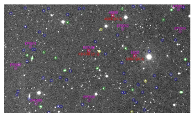
Figure 1.1: A field obtained with INT-WFC on February 28, 2012. Ten asteroids were identified (marked with pink), from which only three were known at the moment of the observation. The size of the field is (15 arcmin x 15 arcmin)

In January 1801, the abbot Giuseppe Piazzi discovered Ceres, a small body at just the right distance. In 1802 Heinrich Olbers discovered Pallas at the same orbital distance. In the follow-ing years, Juno (1804) and Vesta (1807) were discovered also at similar orbital distances with Ceres and Pallas. These bodies were too small to be classified as planets, but the gap was filled. At the beginning of the XIX century, only comets were known to be small objects orbiting the Sun, but they appear like diffuse objects. Herschel, one of the most known astronomers at that time called these objects (Ceres, Palas, Juno, Vesta) asteroids (from Greek "asteroeides"). In this way it was underlined their different appearance - point sources ("star-like") unresolved by the telescopes, compared with the comets which show extended comas.

The first theory of the origin of asteroids, was developed by Olbers in 1803, who suggested that they are fragments of a planet that had been broken to pieces and additional fragments will be found. This prediction became popular, while other asteroids were discovered orbiting at the same solar distance. With the increasing number of these new findings the hypothesis that they could be fragments of an exploded planet became very popular.

In the middle of the 20th century Otto Johannes Schmidt proposed that asteroids represented an arrested stage of planet formation and have never been assembled into a large body. This is now the most plausible hypothesis.

The apparition of photography, offered new means for finding new asteroids. The method consists in comparison of photographic films of the same region of the sky taken at different time intervals. The vast majority of the objects recorded on films were stars and galaxies and

their images were located in the same relative positions on all photographic films. Because a moving asteroid would be in a slightly different position on each picture exposure and the background stars and galaxies were not, it could be identified.

Nowadays the charge coupled devices (CCD) are used instead of photography. While, the CCD technology is more sensitive and accurate than the older photographic methods, the mod-ern discovery technique itself is rather similar. Separated by several minutes, three or more CCD images are taken of the same region of the sky. These images are then compared to see if any asteroid has systematically moved to different positions on each of the separate images (Fig. 1.1).

For a newly discovered object, the separation of the asteroid location from one image to another, the direction it appears to be traveling, and its brightness allow to estimate its orbital characteristics and roughly its size. For example, an object that appears to be moving very rapidly from one image to the next one, is almost certainly very close to the Earth. Computer-aided analyses of the CCD images have replaced the older, manual techniques for all the current asteroid search programs.

Fig. 1.1 shows a field obtained with INT-WFC (Isaac Newton Telescope, Wide Field Cam-era) on the night of February 28, 2012. Ten asteroids could be identified in this field by taking consecutive images at an interval of five minutes. At the moment of the observation only three of the identified asteroids were known.

Thanks to this technological development, during the last decades the total numbers of the asteroids discovered had grown exponentially. Among the most important surveys dedicated to asteroid detection (particularly to Near Earth Asteroids) are those leaded by the United States (CSS, LINEAR, Spacewatch, LONEOS and NEAT) which have been using large field, mostly 1m class telescopes. In the Europe the most important programs were: ASIAGO/ADAS in Italy and Germany, CINEOS in Italy, KLENOT in the Czech Republic, NEON in Finland.

An example of successfully observing run is the one performed by [Boattini et al., 2004]. During two short runs at ESO (European Southern Observatory) LaSilla, they employed the MPG (Max Planck Gesellschaft) 2.2m telescope as a search facility, and the NTT (New Tech-nology Telescope) 3.5m as a follow-up telescope to survey faint asteroids beyond 22 magnitude, for three observing nights. The authors observed about 700 Main Belt asteroids as faint as V 22 magnitude. They exposed between 60s and 150s in the R(red) band.

To conclude this section, as of August 13, 2012 there are 588,219 observed asteroids from which 333,841 have the orbits well determined (as a consequence they were numbered)2.

1.3 Distribution and diversity of asteroids

Asteroids are often grouped according to their orbital parameters. Fig. 1.2 shows the distribu-tion of the asteroids as a funcdistribu-tion of their heliocentric distance. The majority of asteroids are 2_{http://www.naic.edu/~nolan/astorb.html}

36 CHAPTER 1. WHY ASTEROIDS? (a) (b) 123 425 523 623 123 425 523 623

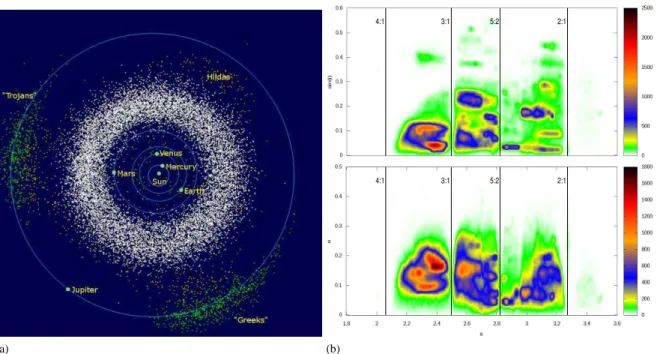
Figure 1.2: a) The position of asteroids in the inner part of the Solar System (Source: http://en. wikipedia.org/). b)The distribution of asteroids in a representation (a,e)- bottom and (a,sini) - top, a is the semi-major axis and i the inclination [Nedelcu, 2010].

located in the Main Belt, at heliocentric distances between 2.1 and 3.3 AU3 (these are called Main Belt Asteroids - MBAs). Several gaps and concentrations can be distinguished by plot-ting the distribution versus semi-major axis (Fig. 1.2b). These gaps are called Kirkwood gaps and correspond to the locations of resonances with Jupiter (in the Fig. 1.2 there are marked 4:1, 3:1, 5:2, 2:1 resonances). The 3:1 and 5:2 resonances located at 2.5 and 2.82 AU, respec-tively define the boundaries between the inner (2.0 - 2.5 AU), middle (2.5 - 2.82 AU), and outer (2.82-3.3 AU) regions of asteroid belt.

The MBAs have diameters up to_{≈500 km (Pallas, Vesta). Ceres, the largest body from the} Main Belt, which has a diameter of_{≈1000 km is classified as a dwarf planet.}

Inside the Main Belt, several clusters of asteroids could be identified [Birlan & Nedelcu, 2010]. These are called asteroid families and are defined by Zappala et al. [1995] as a group of bodies that are genetically and dynamically linked as a result of a catastrophic event: colli-sion of two bodies followed by the destruction of both target and impactor. Usually, they are identified as groups in the space of orbital proper elements [Milani & Knezevic, 1990]..

According to Minor Planet Center (as of August 2012), a total of 5,188 asteroids were discovered near Jupiter’s Lagrangian points L4(3404 objects) and L5(1784 objects) - Fig. 1.2a.

These objects are called Trojan asteroids. They are characterized by low albedo. The largest body is (624) Hektor with a mean radius_{≈100km [de Pater & Lissauer, 2010]. Several Mars} and Neptune Trojans have also been discovered.

Owing to some mechanisms some of the Main Belt Asteroids have migrated into the inner part of the Solar System [Morbidelli et al., 2002]. These are Near-Earth Asteroids (denoted NEAs), small bodies of the Solar System with perihelion distances q_{≤ 1.3 AU and aphelion} distances Q_{≥ 0.983AU, whose orbits approach or intersect Earth orbit. Dynamical studies} con-firmed the main belt origin for the majority of NEAs population. The transition of a main belt asteroid to NEA class is due to the dynamical perturbations associated with the main belt reso-nances. The most active of these regions acting as escape hatches are theν6 secular resonance and the orbital resonances 3:1, 5:2 and 2:1 with Jupiter situated at 2.5, 2.8 et 3.2 astronomical units. Long term numerical integrations have revealed the source regions of the current NEAs population: 61% originated in the inner region of main belt, 24% in the central and 8% in the outer main belt. Only 6% of NEAs are considered to have a cometary origin. The steady-state model of NEA will require a constant flux of objects with H_{≤ 18 of 800/Myr.}

Depending on their orbital parameters, NEAs are subdivided into Amors (1.016< q < 1.3

AU), Apollos (a_{≥ 1.0 AU; q ≤ 1.016 AU), Athens (semi-major axe a < 1.0 AU; Q ≥ 0.983} AU), and Atiras (Q< 0.983 AU).

Potentially Hazardous Asteroids (PHAs) are currently defined based on parameters that measure the asteroid’s potential to make threatening close approaches to the Earth. All as-teroids with an Earth minimum orbit intersection distance (MOID) smaller than 0.05 AU and an absolute magnitude (H) of 22.0 or brighter are considered PHAs [Milani et al., 2000]. A sub-category of these asteroids are virtual impactors (VIs), objects for which the future Earth impact probability is non-zero according to the actual orbital uncertainty [Milani & Gronchi, 2010].

One of the most important aspects related to the NEAs is their accessibility to be inves-tigated by the spacecrafts. Some of them require less propulsion in order to be encountered by spacecraft than that for the Moon, making them ideal mission targets. This enables their scientific study and the detailed assessment of their future use as space resources.

In the last fifty years different observing programs dedicated to asteroids have shown a large diversity in their properties. Several physical properties like diameter, albedo, shape could be deduced from light-curve analysis, radar observations, and polarimetry. The asteroid composi-tion could be inferred through spectroscopic observacomposi-tions. Based on this type of observacomposi-tions, different taxonomic categories were defined with the purpose to roughly correlate the surface compositions of different objects. The first identified types were S (stony - based on the re-semblance with stony meteorites), C (rere-semblances with carbonaceous chondrite meteorites), M (metallic), and E (enstatite achondrite). As a consequence of this taxonomic classification it was discovered the correlation between taxonomic classes and heliocentric distances. The more thermally processed, metamorphic and igneous asteroids classes (E, S, M) are usually found in the central and inner regions of the main belt while the outer regions are dominated by the primitive, relatively unaltered asteroids types. This correlation is rooted in the original

38 CHAPTER 1. WHY ASTEROIDS?

heterogeneity of the protoplanetary disk at the time when the accretion of asteroids started. These taxonomic classes emerged as more and more asteroids observations were available, such that the modern taxonomies (e.g. Bus-DeMeo [DeMeo et al., 2009]) contain more than 20 classes.

From the point of view of their geological evolution, asteroids could be described by three broad categories: primitive, partially melted, and differentiated. Primitive objects are mainly made of silicates, carbon, and organics and some are similar to CI and CM meteorites. Olivine, pyroxene and metal are the main constituents of asteroids partially melted, or at least thermally altered. Remnants of disrupted differentiated bodies include basaltic types, nearly-pure olivine, and metallic bodies, that represent pieces of the crust, mantle, and core [DeMeo, 2010].

1.4 Asteroid brightness and albedo

The apparent magnitude of asteroids depends on geometric parameters (Earth-object distance, Sun-object distance and phase angle) and on the physical and optical properties of the body (size and albedo). The absolute magnitude takes into account only the body intrinsic properties. For asteroids it is defined as being the apparent magnitude if the body were at 1 AU from both the observer and the Sun as seen at phase angleφ = 0. This is an analytical definition because

no geometrical point can satisfy the three conditions at the same time. It can be computed from astrometric and photometric observations with the formula:

H= mv+ 2.5 · log

Φ

r_·∆ (1.2)

where H is the absolute magnitude, mv is apparent magnitude,Φis the phase integral (integra-tion of reflected light; a number in the 0 to 1 range), r is the heliocentric distance (measured in AU), and∆is Earth-object distance (measured in AU) [Magrin, 2006].

The relation between the absolute magnitude and the body physical properties is:

log(pv· D2) = 6.259 − 0.4 · H (1.3)

where D is the diameter of the body expressed in km and pvis the geometrical albedo [Magrin, 2006].

The geometric albedo can be thought of as the amount of radiation reflected from a body relative to that of a flat diffuse surface which is a perfect reflector at all wavelengths (called Lambertian surface) [de Pater & Lissauer, 2010].

1.5 My contribution to asteroids discovery

My contribution to asteroids discovery can be divided in two parts: 1) the observing campaigns in which I was involved and 2) the data-mining of archives for asteroids randomly appearing in

the fields.

Together with my colleagues, I participated to the following observing campaigns for dis-covery, follow-up and recovery of asteroids (in particular for NEAs):

• March, 03 2010; Isaac Newton Telescope (INT) 2.5m, Roque de Los Muchachos

Obser-vatory (ORM) in La Palma (Canary); Data reduction and measurements;

• April 19, 2010; Telescope - T120 Obsv. de Haute Provence (France); Data reduction and

measurements of NEAs;

• November 15-19, 2010; Telescope - T120 Obsv. de Haute Provence (France); On site

mission (observer, data reduction and measurements);

• March 01-04, 2011; T1m, Pic du Midi (France); On site mission (observer, data reduction

and measurements);

• June 03-04, 2011; Blanco 4m - Cerro Tololo, Chile; Data reduction and measurements; • November 16-24, 2011; T1m, Pic du Midi (France); On site mission (observer, data

re-duction and measurements);

• February 25 - 28, 2012; Isaac Newton Telescope (INT) 2.5m, Roque de Los Muchachos

Observatory (ORM) in La Palma (Canary); On site mission (observer, data reduction and measurements);

Figure 1.3: The flowchart of Mega-Precovery [Vaduvescu et al., 2012].

Despite some recent data mining efforts, the vast collection of CCD images and photo-graphic plate archives still remains insufficiently exploited. Considering this point, I was in-volved in the design of a software project for data mining worldwide image archives for poorly known asteroids called MegaPrecovery.

We designed Mega-Precovery [Vaduvescu et al., 2012], with the aim to fasten and target the search of one or some few important objects, such as PHAs or VIs. Given this, we propose to search very large collections of archives for images which include one or few selected known asteroids in their field. There are two components of this project:

40 CHAPTER 1. WHY ASTEROIDS?

Mega-Archive - the database which includes the individual instrument archives, namely the

observing logs for their science CCD images or plates available from a collection of in-struments and telescope around the globe. The Mega-Archive is an open project allowing other instrument archives to be added later for exploration by anybody who would like to contribute. As of March 2012, the Mega-Archive counts about two million images from 20 instrument archives available for search via Mega-Precovery. This include all ESO imaging instruments, the INT WFC, CFHTLS, Subaru Suprime-Cam, Blanco Mosaic-2 and AAT WFI archives;

Mega-Precovery software 4 for data mining the Mega-Archive for the images containing one or a more desired catalogued object (NEAs, PHAs or other asteroids) included in a local daily updated MPC database. The Mega-Precovery software is written in PHP, being embedded on the EURONEAR website as a public access application under the Observing Tools section. The flowchart of the project is given in Fig. 1.3.

The output of Mega-Precovery consists in a list including the images and the corresponding CCD number predicted to contain the queried object(s). The results are displayed both in the web interface (visible only at the end of the run) and sent via e-mail to the user (in case this option was selected). The user can search the images in the online instrumental archive, then download, inspect and measure the data related to this asteroid according to his/her own scientific interest (astrometry, photometry, etc).

Inside EURONEAR team [Vaduvescu et al., 2012], I searched for randomly appearances of known Near Earth Asteroids (NEAs) and Potentially Hazardous Asteroids (PHAs) in ES-O/MPG WFI(Wide Field Imager) and INT WFC archives (these are two wide field 2m class telescope ). A total of 152 asteroids (108 NEAs and 44 PHAs) were identified and measured on 761 images and their astrometry was reported to Minor Planet Center (MPC). Both recov-eries and precovrecov-eries (apparitions of the object in the images before official discovery) were reported, including prolonged orbital arcs for 18 precovered asteroids and 10 recoveries, plus other 124 recoveries.

All the astrometric measurements were submitted to Minor Planet Centerhttp://www.

minorplanetcenter.org/iau/mpc.html. These measurements appear in 12 Minor

Planet Circulars and 21 Minor Planet Electronic Circulars: (79530, 1 (2012); 78894, 9 (2012); 78437, 11 (2012); 77699, 2 (2012); 77266, 11 (2011); 77265, 3 (2011); 77173, 6 (2011); 75198, 5 (2011); 74036, 3 (2011); 72456, 4 (2010); 70198, 9 (2010); 69303, 1 (2010)); (2012-E19 (2012); 2012-D102 (2012); 2012-D82 (2012); W52 (2011); W45 (2011); 2011-W44 (2011); 2011-W33 (2011); 2011-W29 (2011); 2011-W28 (2011); 2011-W27 (2011); 2011-W25 (2011); 2011-W22 (2011); 2011-W12 (2011); 2011-E19 (2011); 2011-E14 (2011); 2011-E13 (2011); 2011-E12 (2011); 2011-E11 (2011); 2010-W13 (2010); 2010-W12 (2010); 2010-W11 (2010)). An example of such circular is given in Fig. 1.4.

2

Why spectroscopy?

Much of the knowledge about the Univers came from the study of electromagnetic radiation received from the cosmic bodies. The most important method to study the electromagnetic radiation is spectroscopy.

This chapter introduces the theory behind the application of spectroscopy in astronomy. A short description of the basic components of a spectrometer (the prism and gratings) is made. The transparency of the Earth atmosphere as a function of wavelength is presented. A simple example of the way in which the properties of celestial bodies could be studied using spectroscopy is shown. The chapter ends by outlining the principles for applying spectroscopy in asteroid studies.

Spectroscopy is one of the most powerful scientific tools for studying the nature. The study of celestial bodies using spectroscopy connects astronomy with fundamental physics at atomic and molecular levels.

The beginning of spectroscopy applied to celestial bodies could be traced back to early nineteenth century with the discovery of dark lines in the solar spectrum by W. H. Wollaston in 1802 and J. von Fraunhofer in 1815. Fraunhofer did not know what is the cause for the dark lines he observed besides the well known characteristic colors of the rainbow. However, he catalogued the exact wavelength of each dark line and today these are still known as Fraunhofer

lines.

On the contrary, in the same period the positivist French philosopher Auguste Comte noted referring to celestial bodies: "We will never know how to study by any means the chemical composition, or their mineralogical structure".

Performing similar observations using light from brightest stars, Fraunhofer concluded that most of the spectral features are somehow related to the composition of the object he observed [Tennyson, 2005]. The physical explanation came later, with the development of quantum mechanics: the dark lines at discrete wavelengths arise from the absorption of energy by the atoms or the ions in the star atmosphere.

Nowadays, the laboratory spectroscopic studies of different chemical components provide the basis for interpreting astronomical spectra. There is a direct connection between the phys-ical parameters of a celestial body and the information that can be obtained by observing its spectrum. By carefully analyzing the spectra it is possible to obtain information about the

com-44 CHAPTER 2. WHY SPECTROSCOPY?

position of the object being observed, its temperature and its internal pressure or density, its motion relative to the Earth, and the presence of a magnetic field.

2.1 Diffraction gratings and prisms

There are several methods that can be used to separate the light into its component wavelengths. The simplest way is to use broad band filters before the detector in order to isolate different spectral regions. This method is called photometry and is considered as a separate subject from the spectroscopy.

Spectral resolution (or resolving power) is defined as the fraction of the wavelength -∆λ, that can be resolved relative to that of the operating wavelength -λ (Eq. 2.1). in general, the spectroscopy is considered to involve spectral resolutions higher than 50.

R= λ

∆λ (2.1)

The astronomical spectrometers are devices that measure the amount of radiation coming from the celestial bodies at different wavelengths. To split the light into its component wave-length, astronomers can use diffraction gratings, prisms, Fabry-Pérot etalons and Fourier trans-form spectroscopes. Bellow are summarized the main characteristics of diffraction gratings and prisms which were used during different observations that I performed.

The diffraction grating generally consists of a large number N, of parallel slits separated by

opaque spaces of comparable dimensions. Producing the spectra with the diffraction gratings involves the interference of N waves and the diffraction on slit phenomena [Cristescu, 2004]. The distribution of intensity of the radiation in the diffraction pattern is described by the formula Eq. 2.2. I= I0_· " sinπbsin_λ θ πbsinθ λ #2 · " sinNπ(b+d)sin_λ θ sinπ(b+d)sin_λ θ #2 (2.2) where d is the size of opaque spaces, b is the size of the slit, θ is the angle between a cer-tain direction and the normal to the grating and I0 is the total intensity passing through a slit

[Cristescu, 2004]. The minima and the maxima position depend on the wavelength and on the diffraction grating parameters (b and d).

By increasing the number N of slits, the interference fringes become sharpest. Two wave-lengths (λ andλ+∆λ) could be barely separated, if the minimum of the diffraction pattern corresponding toλ is in the same position as the bright fringe corresponding to λ+∆λ for the same diffraction order m. From this condition it can be computed the spectral resolution

R_{= N · m. Thus the chromatic resolving power is proportional to the total number of slits and}

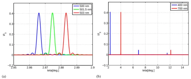
it is higher in the higher orders. In Fig. 2.1 are shown the diffraction patterns obtained using a diffraction grating having b= d = 5µm and N= 1000.

(a) 2.85 2.86 2.87 2.88 2.89 2.9 −0.1 0 0.1 0.2 0.3 0.4 teta[deg.] I/I0 500 nm 501.5 nm 503 nm (b) 2 4 6 8 10 12 14 −0.1 0 0.1 0.2 0.3 0.4 teta[deg.] I/I0 400 nm 700 nm

Figure 2.1: The diffraction pattern produced by a diffraction grating having b= d = 5µm and N=1000. Different

wavelengths are considered.

It can be computed by deriving Eq. 2.3.

λ = d· sinθ

m (2.3)

In practice most gratings use mirrors in place of the slits. On a well-polished surface of a metal, very thin, parallel grooves are drawn. The waves reflected from these grooves behave exactly as the transmitted waves in the case of the transmission gratings. They can be designed such that the main part of the incoming radiation is diffracted selectively on a given order. Because a blaze of light is seen when the grating is viewed at the correct angle, this is called blazed grating [Cristescu, 2004].

The prism acts as a disperser through the effect of differential refraction. This follows from

the fact that the refractive index of a material depends on the wavelength. This dependence can be described by the empirical Hartmann formula - Eq. 2.4.

n_{λ ≈ A +} B

λ−C (2.4)

where A, B, C are the Hartmann constants for a particular material [Kitchin, 1995]. The spectral resolution of a prism is given by:

R_≈ ABL

q

1_{− 0.25n}2_λ

(λ_−C)2 (2.5)

where L is the length of the face of the prism. For a typical prism used in astronomy made of a dense flint and a side length of 10 cm, the spectral resolution could be up to 15,000 [Kitchin, 1995]. Compared to the diffraction gratings which can have higher spectral resolution, this is one of the disadvantages of prisms.

46 CHAPTER 2. WHY SPECTROSCOPY?

Figure 2.2: The atmospheric transmission above Mauna Kea for the wavelength ranges 0.9 - 2.7µm with a water vapor column of 1.6 mm and an air mass of 1 (Source:http://www.gemini.edu/?q=node/10789).

several other components into the instrument called spectrometer. Usually, the designs of spec-trometers incorporate the following basic components: an entrance slit to reduce the overlap between adjacent wavelengths and to reduce the background noise, collimators to produce par-allel beams of light, a dispersive element, a focusing element to produce focused images of the slit for different wavelengths of the spectrum, and a detector.

2.2 Spectroscopy and atmospheric transparency

The observation of celestial bodies using different types of ground-based telescopes is possible in the regions of electromagnetic spectrum for which the atmosphere is transparent. There are two spectral windows which allow the observation: the optical (V) up to the mid-infrared(the near-infrared 0.8 - 2.5µm interval is denoted as NIR) and the radio one. The X-rays and ultra-violet wavelengths are blocked due to absorption by ozone and oxygen, while the far infrared radiation is blocked mainly due to absorption by water and carbon dioxide.

While in the optical wavelength region the atmosphere is almost completely transparent, in the near-infrared there are absorption bands of water vapors making some regions like 1.4-1.5

µm and 1.8-2.0µm poorly transparent (Fig. 2.2). Because of the effects of the atmosphere, ob-servations with space telescopes, such as the Hubble and Spitzer telescopes, are very valuable. Another important difference between the V and NIR spectral intervals is the fact that the sky is brighter in the NIR region. For example in the J, H, K filters1 the estimated sky back-ground has 15.7, 13.6, respectively 13 mag/arcsec2. Additional, important variations of the sky background could be observed in the intervals of tens of arc minutes of the sky.

These issues in the NIR part require additional observing techniques and processing methods (described in Chapter 4) comparing to observation in the V part of the spectrum.

2.3 A simple application

Bellow is described a simple application to exemplify the basic method for obtaining spectra of celestial bodies. It concerns an emission spectrum studied in the V region using a small telescope. Additional details regarding this spectral observation can be found in Popescu et al. [2012a].

An easy way to obtain spectra of celestial bodies is to use a prism or a transmission grating in front of a telescope objective. Depending on the equipment used, the sky quality on the observing moment and data reduction procedures, the limiting magnitude could be pushed up to V = 15 in low resolution mode, with a small telescope (principal mirror diameter below 50 cm).

Together with my colleagues, I carried out observations with telescopes having the diam-eter of principal mirror between 200-300 mm and a diffraction grating having 100 lines/mm [Popescu et al., 2012a]. Since promising results were obtained both for stars and for the quasar 3C273 we took the challenge to observe the quasar PG1634+706 that has and apparent magni-tude V=14.7. The purpose was to identify the emission lines in its spectrum and to calculate their redshift. For this run we used a Celestron C8-NGT telescope, which is a Newtonian type having the primary mirror of 200 mm and a focal length of 1,000 mm, which means a focal ratio f/5. It is used on a AS-GT (CG-5 GoTo) equatorial mount allowing automated tracking of the object. For image recording we used An ATIK 314L+ CCD (charge coupled device) camera having 1.45 Megapixels (a matrix of 1391x1039 pixels), each pixel being a square -6.45 x -6.45µm (chip size - 8.98 x 6.71mm). This camera has a resolution of 16 bits.

The spectrum of PG1634+706 was obtained using a Star Analyser 100 - a high efficiency 100 lines/mm transmission diffraction grating, blazed in the first order. It was mounted in a standard 1.25 inch diameter threaded cell which is compatible with the telescope and CCD camera. A rough calibration of the system can be estimated according to the designer formula adapted to our system (Eq. 2.6):

Dispersionestim[

nm pixel] =

6.45

d[cm] (2.6)

where d is the distance between grating and CCD. The optical design allowed a resolution around 1.5nm. A precise calibration was made using known lines identified in the spectrum of a bright star. The software used for data acquisition was Artemis Capture.

The observations were carried out at 2011-08-05.089 (UT) in a low light pollution area (V˘alenii de Munte - România). The object has the equatorial coordinates RA = 16h34m29s and DEC =+70o31′32”. At the observing moment the object had an air mass of 1.17. The final