HAL Id: hal-01395833
https://hal.archives-ouvertes.fr/hal-01395833v4
Submitted on 8 Dec 2016
HAL is a multi-disciplinary open access archive for the deposit and dissemination of sci-entific research documents, whether they are pub-lished or not. The documents may come from teaching and research institutions in France or abroad, or from public or private research centers.
L’archive ouverte pluridisciplinaire HAL, est destinée au dépôt et à la diffusion de documents scientifiques de niveau recherche, publiés ou non, émanant des établissements d’enseignement et de recherche français ou étrangers, des laboratoires publics ou privés.
Truncated Conjugate Gradient (TCG): an optimal
strategy for the analytical evaluation of the many-body
polarization energy and forces in molecular simulations
Félix Aviat, Antoine Levitt, Benjamin Stamm, Yvon Maday, Pengyu Ren, Jay
W. Ponder, Louis Lagardere, Jean-Philip Piquemal
To cite this version:
Félix Aviat, Antoine Levitt, Benjamin Stamm, Yvon Maday, Pengyu Ren, et al.. Truncated Conjugate Gradient (TCG): an optimal strategy for the analytical evaluation of the many-body polarization energy and forces in molecular simulations. Journal of Chemical Theory and Computation, American Chemical Society, 2017, 13 (1), pp.180-190. �10.1021/acs.jctc.6b00981�. �hal-01395833v4�
Truncated Conjugate Gradient: An Optimal Strategy for the
Analytical Evaluation of the Many-Body Polarization Energy and
Forces in Molecular Simulations
Fe
́lix Aviat,
†Antoine Levitt,
‡Benjamin Stamm,
¶,§Yvon Maday,
∥,⊥,#Pengyu Ren,
■Jay W. Ponder,
△Louis Lagarde
̀re,*
,∇,†and Jean-Philip Piquemal*
,†,⊥†Laboratoire de Chimie Théorique, UPMC Université Paris 06, UMR 7617, F-75005, Paris, France
‡Inria Paris, F-75589 Paris Cedex 12, Université Paris-Est, CERMICS (ENPC), Marne-la-Vallée, F-77455, France ¶MATHCCES, Department of Mathematics, RWTH Aachen University, Schinkelstraße 2, D-52062 Aachen, Germany §Computational Biomedicine, Institute for Advanced Simulation IAS-5 and Institute of Neuroscience and Medicine INM-9,
Forschungszentrum Jülich, Jülich, 52425, Germany
∥Laboratoire Jacques-Louis Lions, UPMC Université Paris 06, UMR 7598, F-75005, Paris, France ⊥Institut Universitaire de France, Paris Cedex 05, 75231, France
#Division of Applied Maths, Brown University, Providence, Rhode Island 02912, United States
■Department of Biomedical Engineering, The University of Texas at Austin, Austin, Texas 78712, United States
△Department of Chemistry, Washington University in Saint Louis, Campus Box 1134, One Brookings Drive, Saint Louis, Missouri
63130, United States
∇Institut du Calcul et de la Simulation, UPMC Université Paris 06, F-75005, Paris, France
ABSTRACT: We introduce a new class of methods, denoted as Truncated Conjugate Gradient(TCG), to solve the many-body polarization energy and its associated forces in molecular simulations (i.e. molecular dynamics (MD) and Monte Carlo). The method consists in afixed number of Conjugate Gradient (CG) iterations. TCG approaches provide a scalable solution to the polarization problem at a user-chosen cost and a corresponding optimal accuracy. The optimality of the CG-method guarantees that the number of the required matrix-vector products are reduced to a minimum compared to other iterative methods. This family of methods is non-empirical, fully adaptive, and provides analytical gradients, avoiding therefore any energy drift in MD as compared to popular iterative solvers. Besides speed, one great advantage of this class of approximate methods is that their accuracy is systematically improvable. Indeed, as the CG-method is a Krylov subspace method, the associated error is monotonically reduced at each iteration. On
top of that, two improvements can be proposed at virtually no cost: (i) the use of preconditioners can be employed, which leads to the Truncated Preconditioned Conjugate Gradient (TPCG); (ii) since the residual of the final step of the CG-method is available, one additional Picard fixed point iteration (“peek”), equivalent to one step of Jacobi Over Relaxation (JOR) with relaxation parameterω, can be made at almost no cost. This method is denoted by TCG-n(ω). Black-box adaptive methods to find good choices of ω are provided and discussed. Results show that TPCG-3(ω) is converged to high accuracy (a few kcal/ mol) for various types of systems including proteins and highly charged systems at thefixed cost of four matrix-vector products: three CG iterations plus the initial CG descent direction. Alternatively, T(P)CG-2(ω) provides robust results at a reduced cost (three matrix-vector products) and offers new perspectives for long polarizable MD as a production algorithm. The T(P)CG-1(ω) level provides less accurate solutions for inhomogeneous systems, but its applicability to well-conditioned problems such as water is remarkable, with only two matrix-vector product evaluations.
1. INTRODUCTION
In recent years, the development of polarizable forcefields has led to new methodologies incorporating more physics. There-fore, higher accuracy in the evaluation of energies can be achieved.1 Indeed, the explicit inclusion of the many-body polarization energy offers a better treatment of intermolecular
interactions, with immediate applications in various fields of application ranging from biomolecular simulations to material science. However, adding polarization to a force field is
Received: October 6, 2016
Published: November 22, 2016
Article
pubs.acs.org/JCTC
© XXXX American Chemical Society A DOI:10.1021/acs.jctc.6b00981
J. Chem. Theory Comput. XXXX, XXX, XXX−XXX
associated with a significant increase of the overall computational cost. In that context, various strategies have been introduced, including Drude oscillators,2 fluctuating charges,3 Kriging methods,4 and induced dipoles.1,5 Among them, the induced dipole approach has been shown to provide a good balance between accuracy and computational efficiency, and can be implemented in a scalable fashion.6
One issue with this approach is the mandatory resolution of a set of linear equations the size of which depends on the number of atoms (or polarizable sites). In practice, for the large systems of interest of force fields methods, a direct matrix inversion approach using the LU or Cholesky decomposition is not computationally feasible because of its cubic cost in the number of atoms. Luckily, iterative methods provide a remedy. We showed in a recent paper6,7 that techniques such as the Preconditioned Conjugate Gradient (PCG) or the Jacobi/Direct Inversion of the Iterative Subspace (JI/DIIS) were efficient for large scale simulations as they offer the possibility of a massively parallel implementation coupled to fast summation techniques such as the Smooth Particle Mesh Ewald (SPME).8The overall cost is then directly proportional to the number of iterations necessary to achieve a good convergence. In that context, predictor-corrector strategies have been introduced to reduce this number using the information on the previous time-steps.9,10 Extended Lagrangian formulations inspired by efficient ab initio methods have also been introduced in order to limit the computational cost, but they require additional thermostats.11In practice, iterative methods are now standard but suffer from energy conservation issues due to their nonanalytical evaluation of the forces. Moreover, force fields are optimized to reach a precision for 10−1to 10−2kcal/mol in the polarization energy. Such a precision can easily be reached using a convergence threshold of 10−3 to 10−4 Debye on the induced dipoles. However, when using iterative schemes, one needs to enforce the quality of the nonanalytical forces in order to guarantee the energy conservation. Hence, a tighter convergence criterion of 10−5to 10−7Debye must be used for its computation. This leads to a very significant increase of the number of iterations. Overall, this additional computational cost is not linked to the accuracy of the polarization energy but only ensures the numerical stability of the MD scheme. In that context, in their 2005 seminal paper12 (see also ref. 13), Wang and Skeel postulated that another strategy would be possible if one could offer a method allowing analytical derivatives and therefore avoiding by construction the risk of loss of energy conservation (i.e. the drift). Such a method would be associated with afixed number of iterations and could extend the applicability of polarizable simulations. Wang explored such strategies based on modified Chebyshev polynomials but noticed that even if the intended analytical expression was obtained, it offered little accuracy compared to fully converged iterated results. In that context, Simmonett et al.14,15 recently proposed to revisit this assumption of a perturbation approach evaluating an approximated polarization energy denoted as ExPT. They proposed a parametric equation offering analytical derivatives and a good accuracy for some class of systems. However, the parametric aspect of the approach limits its global applicability to other types of systems. The purpose of this paper is to introduce a nonempirical strategy based on the same goals: analytical derivatives in order to guarantee energy conservation, limited number of iterations and reasonable accuracy.
We will first present the variational formulation of the polarization energy and the associated linear system. Then, we
will look at iterative methods that are commonly used to solve it and discuss how they can cause problems in molecular simulations. Following this, we will describe two classes of iterative methods, the fixed point methods and the Krylov methods, and see how one can compute the polarization energy and its associated forces analytically (therefore avoiding the energy drift mentioned above). Finally, we will show some numerical results and discuss the accuracy of the new methods. 2. CONTEXT AND NOTATIONS
In the context of forcefields, several techniques are used in order to take polarization into account. Everything that will be presented in this paper concerns the widely used induced dipole model. In this model, each or some of the atomic sites are associated with a 3 × 3 polarizability tensor, so that induced dipoles appear on these sites because of the electricfields created by the permanent charge density and by the other induced dipoles.
2.1. Notations. In the rest of the paper, we will assume that the studied system consists ofN atoms, each of them bearing an invertible 3× 3 polarizability tensor αi. We will denote byE⃗ithe
electricfield created by the permanent density of charge on site i, and byμ⃗ithe induced dipole on sitei. The 3N vectors collecting
these vectors will respectively be noted E andμ. Furthermore, for i ≠ j, we will denote by Tijthe 3× 3 tensor representing the
interaction between theith and the jth induced dipole, so that Tijμ⃗jis the (possibly damped) electricfield created by μ⃗jon sitei.
We are now able to define by blocks the so-called polarization matrix of the system block by block:
α α α = − − − − − − − − ⋱ ⋮ ⋮ ⋮ − − − − − ⎛ ⎝ ⎜ ⎜ ⎜ ⎜ ⎜ ⎜ ⎜ ⎞ ⎠ ⎟ ⎟ ⎟ ⎟ ⎟ ⎟ ⎟ T T T T T T T T T T T ... ... ... N N N N N 11 12 13 1 21 21 23 2 31 32 1 2 1
This matrix is symmetric and we assume that it is also positive definite (thanks to the damping of the electric fields at short-range) so that the energy functional defined below has a minimum and“the polarization catastrophe”16is avoided.
2.2. Variational Formulation of the Polarization Energy and the Associated Linear System. Given these notations, one can express the polarization energy of the studied system in the context of an induced dipole polarizable forcefield as follows:
μ μ μ = − E 1 T E 2 T T pol (1)
The dipolesμ of the quadratic energy functional are determined by the first optimality condition in the form of the following linear system: μ = T E (2) so thatfinally: μ = − E 1 E 2 T pol (3)
for the minimizing dipolesμ. The linear system expressed above has to be solved at each time step of a MD trajectory, so that a computationally efficient technique must be used to solve it. Two kinds of methods exist to solve a linear system, the direct ones and the iterative ones. Thefirst approaches, such as the LU or
DOI:10.1021/acs.jctc.6b00981
J. Chem. Theory Comput. XXXX, XXX, XXX−XXX
Cholesky decomposition, yield exact results (up to round-off errors) but their computational cost grows proportionally toN3
and their memory requirements proportionally to N2, making them hardly usable for large systems of biological interest. 3. ITERATIVE METHODS
In contrast, iterative techniques yield approximate results depending on a convergence criterion, but their computional cost is proportional to the number of iterations times the cost of one iteration (dominated by the cost of a matrix-vector product). This implies that the iterative techniques can be used in conjunction with an efficient matrix-vector multiplication method such as the Smooth Particle Mesh Ewald or the Fast Multipoles.8,17
Several issues arise when using an iterative method to solve the polarization energy. The first one is related to the way the associated forces are computed. Indeed, the polarization energy is a function of the induced dipoles and of the atomic positions, so that one can rely on the chain rule to express the total derivative of this energy with respect to the atomic positions. The induced dipoles are then assumed to be completely minimizing Epol so that μ
∂ ∂
Epol
is assumed to be zero, yielding the following expression (that is analogous to the Hellman−Feynman theorem in quantum mechanics): μ μ = ∂ ∂ ∂ ∂ + ∂ ∂ = ∂ ∂ E r E r E r E r d di i i i
pol pol pol pol
(4) As the iterative method for the resolution of the induced dipoles is never perfectly converged, the previous assumption is never perfectly satisfied. Consequently, the forces calculated using this method are not exactly the negative of thefirst derivative of Epol
(eq 3) with respect to the nuclear positions, potentially giving rise to an energy drift in a MD simulation. This is illustrated by the following graph (Figure 1) representing the evolution of the total energy for a water box of 27 molecules, using the (diagonally) PCG with different convergence thresholds, namely 10−3, 10−4, 10−5, 10−6, and 10−7. An initial guess not issued from the past iterations was used, for a short MD simulation of 10 ps, using a time step of 0.25 fs. Such a small time step was used in
order to minimize the numerical error coming from time-integration. One can directly observe the relation between the convergence threshold and the energy conservation.
The second issue is the computational cost of the iterative methods, proportional to the number of iterations times the cost of one iteration. Solving the polarization equations costs usually (depending on the settings of the simulation) more than 60% of the total cost of an MD step. It has already been shown that carefully choosing the iterative techique employed and taking an initial guess μ0 using information from the past (by using predictor guesses9,10) can yield an important reduction of the number of iterations required to reach a satisfactory convergence threshold. Nevertheless, some limitations exist due to the imperfect time reversibilty and volume preservation that they imply. Furthermore, the ability to parallelize the method efficiently also influences the choice of the optimal method.6,7
These issues motivate the derivation of a computationally cheap analytical approximation of the polarization energy in polarizable MD. We aim also for such an approximation to be as close as possible to the exact results (or at least within the accuracy of the force field) so that it would not require a reparametrization of the force fields. For the forces to be analytical, the computation of the induced dipoles must be history free and should therefore avoid the use of predictors. 4. FIXED POINT METHODS AND RELATION WITH ExPT Thisfirst class of methods regroups the fixed point methods, also called stationary methods. In this case, one splits the matrix into two parts in order to re-express the solution of the linear system as afixed point of a mapping associated with the splitting. For the polarization matrix one can re-express T as the sum of its (block-) diagonal and off-diagonal part:
α
= − −
T 1 ; (5)
yielding the following expression of the solutionμ:
μ=α(E+;μ) (6)
whereμ appears as the fixed point of a mapping. Then, Picard’s fixed point theorem18
tells us that starting from any guessμ0and
computing the following sequence of dipoles (denoted by rnthe
residual associated withμn):
μn+1 =αE+α μ; n =μn +αrn (7) we converge toward the solution if ρ(α;)<1, with ρ(M) denoting the spectral radius of a given matrix M. The method that was described above is the Jacobi method and if we had split the matrix between its upper triangular part and the remaining terms, we would have obtained the Gauss−Seidel method.
A direct refinement of the Jacobi method consists in choosing a“relaxation” parameter ω and the following (relaxed) scheme: μn+1 =(1− ω)μn +ω(μn +αrn)=μn +ωαrn (8) which is convergent ifρ(Id− ωαT) < 1. In the rest of the text we
will denote this method as JOR (Jacobi over Relaxation).19,20 One way to get analytical approximations of the polarization energy is to truncate one of these methods at afixed order. One could for example choose to truncate the Jacobi method at some ordern to obtain an analytical approximation to the solutions of the induced dipoles which we rearrange as:
μn =μ(0) + μ(1) +...+μ( )n (9) with
Figure 1.Evolution of the total energy of a water box of 27 molecules computed with PCG and different convergence thresholds (AMOEBA), and with the TPCG2(ωfit) method, withP = diag. The drift on the total
energy is fully related to the polarization contribution, the TPCG2(ωfit)
converges to the 10−7PCG results without any drift.
DOI:10.1021/acs.jctc.6b00981
J. Chem. Theory Comput. XXXX, XXX, XXX−XXX
μ( )n = α(;α)nE (10) which is exactly the formulation of the perturbation theory (PT) method proposed by Simmonett et al.,14even though they follow another reasoning related to perturbation theory. The ExPT method that they propose is then made by truncating this expansion at order two and by using a linear combination ofμ1
andμ3
μExPT = c0 0μ + c1 3μ (11)
in order to provide the following expression for the approximation of the polarization energy:
μ = − E 1 E 2 T pol,ExPT ExPT (12)
The computational cost of this method is then equivalent to making three matrix-vector multiplication and its accuracy is good in many cases but it has the disadvantage of using two parameters that need to be fitted. Simmonett and co-workers recently extended the ExPT technique to higher orders, giving the OPTn class of methods,15that lead to improved results but require even more empirical parameters.
5. KRYLOV METHODS: PRECONDITIONED CONJUGATE GRADIENT
The point of view of the Krylov methods is completely different.21It consists in minimizing some energy functional at each iteration over some growing subspaces.
Starting from some initial guessμ0, let us define the associated residual:
μ
= −
r0 E T 0 (13)
We are now able to define the so-called Krylov subspaces of order ∈
p :
= −
Kp span( , Tr , ...,r0 0 Tp 1r0) (14) We clearly have the following inclusion of spaces:
⊆̲ ⊆̲
K1 K2 ... (15)
Then,μnis determined as the minimum of the energy functional
overμ0+Kp. As one is minimizing at each iteration the energy
functional over some increasing sequence of embedded spaces, the error (as measured by the functional) is necessarily decreasing. One can show that there exists ap ≤ 3N such that the exact solution μ belongs to μ0 + Kp, meaning that these
methods always converge and even provide the exact solution after afinite number of steps, the worst case being when they converge in 3N iterations. In practice, however, only very few iterations are needed to obtain accurate solutions.
The different Krylov methods are determined by the quantity that is minimized over the Krylov subspaces: if one minimizes Epol then one obtains the conjugate gradient (given the
assumption that T is symmetric definite positive), if one minimizes ∥rn∥l2 then one gets the GMRES method21(which
is equivalent to some version of the JI/DIIS22). But many other methods exist, such as the Minres algorithm23 or the BiCG method21for nonsymmetric matrices.
The conjugate gradient algorithm updates three vectors at each iteration: a descent direction, a dipole vector, and the associated residual. These vectors are updated using three scalars that are obtained by making some scalar products over these
vectors. After the following initialization (using here the direct field αE as an initial guess):
μ α μ = = − = ⎧ ⎨ ⎪ ⎩ ⎪ E r E T p r 0 0 0 0 0 (16)
the algorithm reads as follows:
μ μ γ γ γ β β = = + = − = = + + + + + + + + + ⎧ ⎨ ⎪ ⎪ ⎪ ⎪ ⎪ ⎩ ⎪ ⎪ ⎪ ⎪ ⎪ r r p Tp p r r Tp r r r r p r p i i i i T i i i i i i i i i i i T i i T i i i i i T 1 1 1 1 1 1 1 1 (17)
where piis the descent direction at iterationi, μithe associated
dipole vector, and rithe associated residual. The magic of the conjugate gradient algorithm is that this simple recursion scheme still guarantees μi to be the optimum over the entire Krylov-subspace of orderi.
There are several techniques to accelerate the convergence of this algorithm. A widely used strategy is to use preconditioners. Indeed, one can show that the convergence rate of the conjugate gradient, and more generally of Krylov subspace methods, depends on the condition number of the matrix that is being inverted: the lower this number is (it is always greater than 1), the faster the conjugate gradient will converge. In the case of symmetric positive definite (s.p.d.) matrices as the polarization matrix, this number can be expressed such as
κ λ λ = T ( ) max min (18)
whereλmaxandλminare the largest and smallest eigenvalues of the
polarization matrix. A preconditioner is then a matrixP that is ”close” to the inverse of T, such that the matrix P is easily applied to a vector,κ(PT) ≤ κ(T), and κ(PT) is close to 1. The conjugate gradient algorithm is then applied to the matrixPT with PE as a right-hand side. Wefirst chose to use one of the simplest forms of preconditioner: the diagonal or Jacobi preconditioner, in whichP is the inverse of the (block-)diagonal part of the polarization matrix. The advantage of this choice in our context is that multiplying a matrix by a diagonal matrix is computationaly almost free and that the diagonal of T does not depend on the positions of the atoms of the system that is studied. As a consequence, this choice does not complicate the expression of the gradients very much. On the down side, the diagonal of T is not a perfect approximation of it, so that we do not expect the acceleration of convergence to be the highest among the possible choices of preconditioners. This is why we also considered a more efficient preconditioner designed for the polarization problem which we will present below. Wang and Skeel12start from the expression
α α
= −
− −
I
T 1 (d ;) 1 (19)
giving thefirst approximation
α α ≈ + − I T 1 (d ;) (20) DOI:10.1021/acs.jctc.6b00981
J. Chem. Theory Comput. XXXX, XXX, XXX−XXX
which is in fact equivalent to one Jacobi iteration. A second approximation is then made by only considering the interactions within a certain cutoff in the matrix;. A typical value for this cutoff is 3 Å, a value that we also used for our numerical tests presented below. This preconditioner has a bigger impact on reducing the condition number of the polarization matrix than the Jacobi one but it also has a higher computational cost per iteration. This cost is typically a bit less than half a real space matrix-vector product within a Particle Mesh Ewald simulation with usual settings for the value we chose (7 Å cutoff). The parallel implementation of this preconditioner would require additional communications before and after the application of this preconditioner.6 Finally, as it depends on the atoms positions, the expression of the gradients of the associated dipoles would be very involved (therefore in the following sections we will only retain the diagonal preconditionner). To illustrate the different rates of convergence of these iterative methods we plotted inFigure 2their convergence as well as the
one of JI/DIIS wich is described in ref.7(represented by the norm of the increment) as a function of the number of iterations in the context of the AMOEBA polarizable force field for the ubiquitin protein in water. Note that the Jacobi iterations are not convergent in this case and that both the JI/DIIS and the Preconditioned Conjugate Gradient converge twice as fast as the JOR (as supported by the theory, as the convergence rate of JOR depends on the condition number, while the rate of Krylov methods depends on its square root).
We will now explain how to truncate the preconditioned conjugate gradient to get analytical expressions that approximate the polarization energy.
6. TRUNCATED PRECONDITIONED CONJUGATE GRADIENT
Let us define μTCGn, the approximation of the induced dipoles obtained by truncating the conjugate gradient at order n. We immediately have the result that Epol(μ) ≤ Epol(μTCGn) ≤
Epol(μTCGm) ifn ≥ m, with Epolwritten as ineq 1, andμ being the
exact solution of the linear system. In other words, the quality of the approximation is systematically improvable. One can then unfold the algorithm at order one and two. Using the following notations: γ = = = = = = = = − n t t n t t t t n t t n t r r P Tr r P P P Tp P P P T T T 0 0 0 1 0 1 0 1 2 0 1 2 1 2 2 1 3 1 1 2 4 0 1 1 12 0 1 2 3 (21)
one obtains the cumbersome but analytical approximations for the dipoles corresponding to the conjugate gradient truncated at order one and two, thus allowing the derivation of analytical forces that are the exact negative of the gradients of the energy:
μTCG1= μ0 +t r4 0 (22)
μTCG2 =μ0 +(t4+γ1 2t )r0−γ1 4 1t P (23) As in the ExPT approach, one can take the following expression as approximation of the polarization energy:
μ = − E 1 E 2 n n T pol,TCG TCG (24)
Note that both these expressions would be exact if the dipole vectors were exact and that the closer these vectors are to the fully converged dipoles, the closer these energies will be to the actual polarization energy. Indeed, we have: μ μ μ μ μ μ |E ( )−E ( )| = 1 T − E + E 2 1 2 n T T T pol T(P)CG (25) μ μ μ μ |E ( )−E ( )| = 1| T −E | 2 ( ) n T pol T(P)CG (26)
leading to the following inequatlity:
μ μ μ
|E ( )−E ( )| ≤ 1∥ ∥ ·∥ ∥r 2
n l n l
pol T(P)CG 2 2 (27)
These energies are not the expression minimized over the Krylov subspaces at each iteration of the conjugate gradient (CG) algorithm (see eq 1), but they coincide at convergence which should almost be the case if our method is accurate.
These results are naturally extended to the preconditioned conjugate gradient (PCG). One can of course also choose to truncate the (P)CG at a superior order and still be analytical to obtain a more accurate approximation, at the price however of additional computational time, and the analytical expression of the energy and its derivatives will be incrementely more complex, thus cumbersome to implement. In the following section, where numerical results are presented, we will limit ourselves to TCG3 as the highest order of truncation.
Moreover, having chosen an order of truncation of the (P)CG, one can exploit the residual (if it is computed to monitor the accuracy) of the last iteration of the truncated algorithm in order to get closer to the converged value by computing one step of a Figure 2. Norm of the increment as a function of the number of
iterations for different iterative methods (AMOEBA), computed on ubiquitin.
DOI:10.1021/acs.jctc.6b00981
J. Chem. Theory Comput. XXXX, XXX, XXX−XXX
fixed point iterative method. As did Wang and Skeel,12
we will call this operation a peek step. Indeed, manyfixed point iterative methods such as the Jacobi and more generally the JOR only require to know a starting value of the dipoles and the associated residual to be applied at each iteration. Note that the Jacobi method can be seen as a particular case of the JOR method with ω = 1 and that this operation is not computationally expensive, as it only requires a matrix-vector product with a diagonal matrix if the residual is known. As for anyfixed-point method of a linear system, the asymptotic convergence of the JOR method depends on the spectral radius of the iteration matrix. More precisely, the condition
α
ρ(Id−ω T)<1 (28)
guarantees that the JOR method is convergent. Asymptotically, the best convergence rate is obtained with the value ofω that minimizes this spectral radius. One can show that if T is symmetric positive definite, this value is
ω λ λ = + 2 opt min max (29)
λmin and λmax being, respectively, the smallest and largest
eigenvalue ofαT.
As these results are asymptotic, one cannot necessarily expect the associated methods to give the best results if only the so-called peek step is applied, as this depends on the composition of the current approximation (which is in our case provided by the T(P)CG) in the eigenvector-basis of T.
Since we cannot rely on asymptotic results for one iteration, we also explored another strategy that can be of use in cases in which one is particularly interested in the values of the energies, as for example in Monte Carlo simulations. Theωoptbased on the
spectrum intends to further optimize all the modes of the polarization matrix after the (P)CG steps (independently of the actual approximation) and should therefore asymptotically improve both the energy and the RMS. However, other values ofω that take into account the actual approximation can be used to further improve the accuracy. This explains why we tried, starting from one or two iterations of (P)CG, to choose the value ofω that gave the closest approximate polarization energy to the fully converged one. Since the optimal parameter (in this new sense) requires another matrix-vector multiplication, we tried to obtain values of this parameter on thefly by fitting one or several energies against the energies obtained with the fully converged dipoles or a superior truncation of (P)CG. It will be calledωfit.
Starting for example fromμTCG2, and noting:
μTCG2,peek =μTCG2 +ωαr2 (30)
one can see this procedure as a line search: given the starting point μ2, one further tries to optimize the energies along the
parametrized lineμ2+ωαr2forω ∈ .
Once one of these methods is chosen, analytical expressions of the associated forces can be naturally obtained, thus ensuring that the forces are (up to round off errors) the opposite of the exact gradients of the polarization energy, and thus avoiding an energy drift. Gradients of the energies have been derived and are presented in a technical appendix at the end of the manuscript. 7. NUMERICAL RESULTS
7.1. Energy Conservation of the T(P)CGn Approaches. Wefirst emphasize thatFigure 1already displays an important result: the TCGn methods ensure total energy conservation as
they use analytical evaluation of the forces. All further refinements discussed in section 6lead to the same behavior, incremently closer to the reference energy.
7.2. Stability of the Spectrum. Before presenting the complete numerical tests, we analyze here the spectrum of the polarization matrix during a MD simulation. Indeed, as pointed out in the theory section, some refinements of the TCG rely on the extreme eigenvalues of T andαT. We followed the evolution of these eigenvalues during 100 ps of MD. Those tests were made with the Lanczos algorithm since all the matrices we are interested in are symmetric. Indeed, one great advantage of the Lanczos method is that it reduces the computational cost compared to direct methods (such as the one available in the LAPACK library). That way, if direct eigenvalue solvers force the user to compute the full spectrum (i.e all the eigenvalues), Lanczos method allows rapid access to the extreme eigenvalues by constructing a much smaller tridiagonal matrix whose spectrum is close to the one of the original matrix, leading to almost identical extreme eigenvalues that can then be obtained in a few iterations. We observed that in all cases these values are stable over the 100 ps of the MD trajectories as pointed out by Skeel.12This can be seen for S3 and the ubiquitin system in
Figures 3and4. This result motivated our choice to computeωopt
andωfitfor thefirst geometry of our equilibrated systems and to
keep this value for all the others geometries. Both our Lanczos Figure 3. Evolution of the extreme eigenvalues of αT for S3 and ubiquitin.
Figure 4.Evolution ofωoptfor S3 and ubiquitin.
DOI:10.1021/acs.jctc.6b00981
J. Chem. Theory Comput. XXXX, XXX, XXX−XXX
implementation and the energyfitting procedure are fast enough to be used on thefly while being negligeable over a 100 ps MD simulation. In our tests, the adaptive reevaluation of theω’s was nevertheless never required.
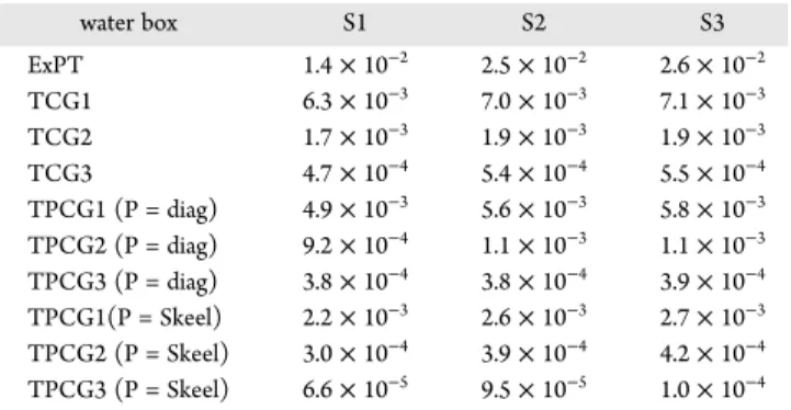
7.3. Computational Details and Notations. In this section, we will present some numerical results from the methods presented above. All the tests presented here were made using the AMOEBA polarizable force field24,25 imple-mented in our Tinker-HP code.26The proposed benchmarks deal with homogeneous and inhomogeneous systems: water clusters and protein in water droplets as well as an ionic liquid system. The three water systems will be called S1, S2, and S3 and contain respectively 27 molecules (81 atoms), 216 molecules (648 atoms), and 4000 molecules (12000 atoms). We chose difficult systems ranging from usual proteins to metalloproteins and highly charged ionic liquids.27 The protein droplets are, respectively, a metalloprotein containing two Zn(II) cations (nucleocapsid protein ncp7) with water (18515 atoms including counterions), the ubiquitin protein with water (9737 atoms), and the dhfr protein with water (23558 atoms). The ionic liquid system is made of [dmim+][Cl−] (1−3 dimethylimidazolium) ions, making it a highly charged system of 3672 atoms with a very different regime of polarization interactions. All the results presented in this section were averaged over 100 geometries that were extracted from a 100 ps MD NVT trajectory (one geometry was saved every picosecond) at 300 K for all systems, except the [dmim+][CL−] at 425 K. The results, that will give indications about the accuracy of the approximate methods compared to the fully converged iterative results, will give two different and complementary aspects of this accuracy. We willfirst compare the polarization energies (in kcal/mol) obtained with dipoles converged with a very tight criterion (RMS of the residual under 10−9) to the ones obtained with T(P)CG. We will then present the RMS of the difference between the fully converged dipole vectors and the approximate methods. This RMS is a good indicator of the quality of T(P)CG forces compared to the reference: the smaller this RMS is, the closer the approximated but analytical forces will be to the reference force.
Tables 1to4describe the water systems andTables 5to8
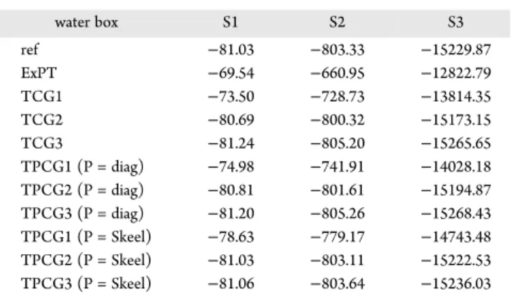
describe the protein droplets and ionic liquid. We will denote by “ref” the results obtained with dipoles converged up to 10−9in
the RMS of the residual; by“ExPT” the results obtained with the method of Simmonnet et al. presented insection 3; by“TCGn” (withn = 1, 2, and 3) the results obtained with the CG truncated at order 1, 2, and 3; by“TPCGn” (P = diag) (with n = 1, 2, and 3) the results obtained with the preconditioned (with the diagonal) CG truncated at order 1,2 and 3; by“TPCGn” (P = Skeel) (with n = 1, 2, and 3) the results obtained with the preconditioned (using Wang and Skeel’s preconditioner) CG truncated at order 1, 2, and 3.
Furthermore, we will present results obtained with different kinds of peek steps. We willfirst denote by TCGn(ω = 1) (with n = 1, 2, and 3) the results obtained with the CG truncated at different orders when a Jacobi peek step is made after the last conjugate gradient iteration. We will also denote by TPCGn (P = diag) the results where the same peek step is made after different numbers of iterations of the PCG with a diagonal preconditioner. We will also denote by TPCGn(P = diag)(ωopt) (withn = 1
and 2) the results obtained with 1 and 2 iterations of diagonally preconditioned CG and a JOR peek step with an“optimal” ωopt
in the sense ofsection 6(that depends whether a preconditioner is used or not).
As explained in the previous section we also explored a strategy where the damping parameter of the JOR step is fitted to reproduce energy values. In the following tables, the damping parameter will be denoted byωfit.
7.4. Numerical Results. Afirst observation to make is that given a particular matrix (preconditioned or not) and with or whithout a JOR peek step, the results are always better in terms of energy and RMS when one performs more matrix-vector products, that is, going to a higher order of truncation. This is naturally explained in the context of the Krylov methods: an additional matrix-vector product increases the dimension of the Krylov subspace on which the polarization functional (seeeq 1) is minimized, and thus systematically improves the associated results. We should also recall here that the functional that is minimized over growing subspaces is not exactly the same as the one we are taking as the polarization energy and that this explains the nonvariationality of some of our results: there are many cases where the energy associated TCG3 is slightly lower than the one associated with the fully converged dipoles (see discussion in
section 6).
We can also see on the numerical tests that using a preconditioner systematically reduces the associated RMS. Concerning the energy, the improvement is less systematic and depends on the type of preconditioner: the diagonal is less accurate than the one described by Wang et al.,12a result that was anticipated.
Nevertheless, preconditioning is important when coupled with a peek step: a combination of any preconditioner with the peek is better than the peek alone. However, concerning the peek itself, one observes a systematic improvement of both RMS and energy Table 1. Polarization Energies of Water Systems
water box S1 S2 S3 ref −81.03 −803.33 −15229.87 ExPT −69.54 −660.95 −12822.79 TCG1 −73.50 −728.73 −13814.35 TCG2 −80.69 −800.32 −15173.15 TCG3 −81.24 −805.20 −15265.65 TPCG1 (P = diag) −74.98 −741.91 −14028.18 TPCG2 (P = diag) −80.81 −801.61 −15194.87 TPCG3 (P = diag) −81.20 −805.26 −15268.43 TPCG1 (P = Skeel) −78.63 −779.17 −14743.48 TPCG2 (P = Skeel) −81.03 −803.11 −15222.53 TPCG3 (P = Skeel) −81.06 −803.64 −15236.03
Table 2. Polarization Energies of Water Systems, Using a Peek-Step water box S1 S2 S3 ref −81.03 −803.33 −15229.87 TCG1(ω = 1) −81.41 −806.83 −15315.13 TCG2(ω = 1) −80.23 −794.49 −15061.22 TCG3(ω = 1) −80.78 −800.83 −15181.55 TPCG1 (P = diag)(ω = 1) −79.88 −791.51 −15001.40 TPCG2 (P = diag)(ω = 1) −80.98 −802.74 −15218.27 TPCG3 (P = diag)(ω = 1) −81.03 −803.27 −15228.74 TPCG1 (P = diag)(ωopt) −78.98 −780.94 −14789.04 TPCG2 (P = diag)(ωopt) −80.95 −802.50 −15213.17 TPCG1 (P = diag)(ωfit) −81.06 −803.42 −15230.10 TPCG2 (P = diag)(ωfit) −81.02 −803.06 −15231.14 DOI:10.1021/acs.jctc.6b00981
J. Chem. Theory Comput. XXXX, XXX, XXX−XXX
with and without preconditioning. In particular this is the case whenω = 1 (Jacobi peek step).
As the spectrum is stable (seesection 7.2), one can use an adaptiveωoptcoefficient computed on one geometry using a few iterations of the Lanczos method. In that case, the energies are slighlty less accurate than the ones obtained with ω = 1. Concerning the RMS, we observe a systematic reduction by a factor 2 for TPCG2 and TPCG3 but not for TPCG1. This occurs because, if the asymptotic coefficient ωoptis the same, the starting
point of the peek step is different and is significantely better for TPCG2 and TPCG3 as additional matrix-vector products have been computed.
The results obtained withωfitafter 1, 2, or 3 iterations of PCG
show that it is possible to stay close to the converged value of the polarization energy with only one or two matrix-vector products and a ω parameter that is only fitted once during a 100 ps dynamic. But we can also see that this is made at the cost of slightly degrading the RMS compared to the results obtained withωoptor withω = 1. Overall, these RMS are of the same order
of magnitude than the ones obtained withωoptandω = 1. This balance between RMS and energy depending on the choice ofω as the relaxation parameter for a JOR peek step can be seen as the choice to favor the minimization of the error along some modes of the polarization matrix: the energy is more sensitive to modes corresponding to large eigenvalues whereas the RMS is sensitive to all of them. Overall, aω = 1 Jacobi peek step tends to improve both RMS and the energy whereas ωopt favors RMS andωfit
favors energies. As we showed, TPCG1 should not be used with a ωoptpeek step but with one corresponding toω = 1 and ωfit, but
all options are open for TPCG2 and TPCG3.
A choice can then be made depending on the simulation that one wants to run. For a Monte Carlo simulation it is essential to have accurate energies: the strategy of using an adaptative parameter (refittable at a negligeable cost) that allows the correct reproduction of the energies with only one or two iterations of the (P)CG would hence produce excellent results. On the other side, during a MD simulation, one wants to get the dynamics right; in this case, choosing the method that minimizes the RMS and thus the error made on the forces may produce improved results. For example, using TPCG2(P = diag)(ωopt) is a good strategy to fulfill this purpose. However, the procedure leading to ωfitonly slightly degrades the RMS and provides RMS far beyond
the usual values for which the force field models are parametrized. One has also to keep in mind that other source of errors exist in MD, such as the ones due to the PME discretization or van der Waals cutoffs, that are larger than the error discussed in this section. Nevertheless, none of the refinements will compete with a full additional matrix-vector product because an additional CG step is optimal. We see clearly that TPCG3(ωfit) reaches high accuracy on both RMS and energies.
Concerning preconditioning, we confirm the very good behavior of the Skeel preconditioner. However, its cost is non-negligible in terms of computations, in terms of necessary communications arising when running in parallel, and in terms of complexity of implementation. We recommend therefore the use of the simpler yet efficient diagonal preconditioner. Overall, possibilities of tayloring TCG approaches are infinite. In practice, one could design more adapted preconditioners combining accuracy and low computational cost.
To conclude, a striking result is obtained for well conditioned systems such as water: computations show that they will require a smaller order of truncation than the proteins to obtain the same level of accuracy.
8. CONCLUSION
We proposed a general way to derive an analytical expression of the many-body polarization energy that approximates the inverse of T using a truncated preconditioned conjugate gradient approach. The general method gives analytical forces, guarantee-ing that they are the opposite of the exact gradients of the energies, parameter free, and can replace the usual many-body polarization solvers in popular codes with little effort. The proposed technique allows by construction a true energy conservation as it is based on analytical derivatives. The method Table 3. RMS of the dipole vector compared to the reference
for water systems
water box S1 S2 S3 ExPT 1.4× 10⁻² 2.5× 10⁻² 2.6× 10⁻² TCG1 6.3× 10⁻³ 7.0× 10⁻³ 7.1× 10⁻³ TCG2 1.7× 10⁻³ 1.9× 10⁻³ 1.9× 10⁻³ TCG3 4.7× 10⁻⁴ 5.4× 10⁻⁴ 5.5× 10⁻⁴ TPCG1 (P = diag) 4.9× 10⁻³ 5.6× 10⁻³ 5.8× 10⁻³ TPCG2 (P = diag) 9.2× 10⁻⁴ 1.1× 10⁻³ 1.1× 10⁻³ TPCG3 (P = diag) 3.8× 10⁻⁴ 3.8× 10⁻⁴ 3.9× 10⁻⁴ TPCG1(P = Skeel) 2.2× 10⁻³ 2.6× 10⁻³ 2.7× 10⁻³ TPCG2 (P = Skeel) 3.0× 10⁻⁴ 3.9× 10⁻⁴ 4.2× 10⁻⁴ TPCG3 (P = Skeel) 6.6× 10⁻⁵ 9.5× 10⁻⁵ 1.0× 10⁻⁴
Table 4. RMS of the Dipole Vector Compared to the Reference for Water Systems, Using a Peek-Step
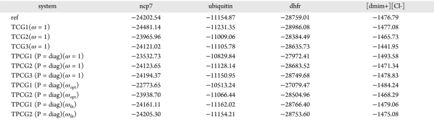
water box S1 S2 S3 TCG1(ω = 1) 3.6× 10⁻³ 3.9× 10⁻³ 3.7× 10⁻³ TCG2(ω = 1) 1.5× 10⁻³ 1.7× 10⁻³ 1.8× 10⁻³ TCG3(ω = 1) 4.6× 10⁻⁴ 4.9× 10⁻⁴ 4.8× 10⁻⁴ TPCG1(P = diag)(ω = 1) 2.2× 10⁻³ 2.6× 10⁻³ 2.7× 10⁻³ TPCG2 (P = diag)(ω = 1) 4.1× 10⁻⁴ 5.0× 10⁻⁴ 5.2× 10⁻⁴ TPCG3 (P = diag)(ω = 1) 1.3× 10⁻⁴ 1.5× 10⁻⁴ 1.6× 10⁻⁴ TPCG1 (P = diag)(ωopt) 2.3× 10⁻³ 2.7× 10⁻³ 2.8× 10⁻³ TPCG2 (P = diag)(ωopt) 3.9× 10⁻⁴ 4.6× 10⁻⁴ 4.7× 10⁻⁴ TPCG1 (P = diag)(ωfit) 2.6× 10⁻³ 3.0× 10⁻³ 3.0× 10⁻³ TPCG2 (P = diag)(ωfit) 5.3× 10⁻⁴ 7.0× 10⁻⁴ 1.0× 10⁻³ Table 5. Polarization Energies of Protein Droplet and Ionic Liquids system ncp7 ubiquitin dhfr [dmim+] [Cl−] ref −24202.54 −11154.87 −28759.01 −1476.79 ExPT −27362.70 −10919.77 −28076.62 −5841.73 TCG1 −21733.63 −9897.22 −25583.50 −1428.35 TCG2 −23922.79 −11031.67 −28463.51 −1420.00 TCG3 −24262.87 −11174.93 −28812.99 −1450.22 TPCG1 (P = diag) −21438.14 −9907.09 −25588.07 −1465.66 TPCG2 (P = diag) −23613.31 −10948.32 −28206.73 −1462.22 TPCG3 (P = diag) −24219.49 −11164.62 −28775.53 −1469.89 TPCG1 (P = Skeel) −22489.55 −10458.44 −27030.86 −1424.49 TPCG2 (P = Skeel) −24056.53 −11090.36 −28637.35 −1469.05 TPCG3 (P = Skeel) −24208.22 −11144.53 −28763.55 −1477.02 DOI:10.1021/acs.jctc.6b00981
J. Chem. Theory Comput. XXXX, XXX, XXX−XXX
minimizes the energy over the (preconditioned) Krylov space which leads to superior accuracy than fixed point inspired methods such as ExPT and associated methods. It does not use any history of the previous steps and is therefore fully time reversible and is compatible with multitimestep integrators.28 The best compromise between accuracy and speed appears to be the TPCG-2 approach that consists of two iterations of PCG with a computational cost of three matrix vector multiplications for the energy (one for the descent direction plus two for the iterations). The analytical derivatives have a cost equivalent to an additional matrix vector product. The overall computational cost is therefore identical to that of the ExPT. We showed that the method allows the computation of potential energy surfaces very close to the exact ones and that it is systematically improvable
using afinal peek step. Strategies for adaptative JOR coefficients have been discussed and allows an improvement of the desired quantities at a negligeable cost. Overall, among all the derived methods, TPCG3(ωfit) provides high accuracy in both energy
and RMS. Concerning the future improvements of the accuracy of the method, one could find dedicated preconditionners improving the efficiency of the CG steps. Nevertheless, the final choice of ingredients will be a trade-off between accuracy, computational cost, and communication cost when running in parallel. We will address this issue in the context of the Tinker-HP package. The TPCGn approaches will be coupled to a domain decomposition infrastructure with linear scaling capabilities, thanks to a SPME8 implementation, which is straightforward in link with our previous work on PCG. Future work will then include validation of the methods by comparing condensed-phase properties obtained using different orders of TCG. Given the level of accuracy already obtained on induced dipoles and energies, we expect the majority of these properties to be conserved by using T(P)CG2 and higher-order methods.
■
TECHNICAL APPENDIXA.1. Analytical Gradients and Polarization Energies for TCG In this section, we will present the analytical derivatives of the polarization energies associated with the polarization energies Epol,TCG1andEpol,TCG2with respect to the positions of the atoms
of the system. The extension to Epol,(P=diag)TCG1 and
Epol,(P=diag)TCG2is straightforward, as is the expressions including
afinal JOR peek step. We don’t report here the expression of the analytical gradients ofEpol,TCG3as it follows the same logic but is
just incremently complex.
These gradients have been validated against the ones obtained withfinite differences of the energies and an implementation of these equations will be accessible through the Tinker-HP Table 6. Polarization Energies of Protein Droplet and Ionic Liquids, Using a Peek-Step
system ncp7 ubiquitin dhfr [dmim+][Cl-]
ref −24202.54 −11154.87 −28759.01 −1476.79 TCG1(ω = 1) −24481.14 −11231.35 −28986.08 −1477.08 TCG2(ω = 1) −23965.96 −11009.06 −28384.49 −1465.73 TCG3(ω = 1) −24121.02 −11105.78 −28635.73 −1441.95 TPCG1 (P = diag)(ω = 1) −23532.73 −10829.84 −27972.41 −1493.58 TPCG2 (P = diag)(ω = 1) −24123.65 −11128.14 −28683.52 −1471.34 TPCG3 (P = diag)(ω = 1) −24194.37 −11150.95 −28749.68 −1478.83 TPCG1 (P = diag)(ωopt) −22773.65 −10513.24 −27079.47 −1484.24 TPCG2 (P = diag)(ωopt) −23938.70 −11066.44 −28504.96 −1468.29 TPCG1 (P = diag)(ωfit) −24161.11 −11162.02 −28766.40 −1479.06 TPCG2 (P = diag)(ωfit) −24205.30 −11154.21 −28753.60 −1475.08 Table 7. RMS of the Dipole Vector Compared to the
Reference for Protein Droplets and Ionic Liquids
water box ncp7 ubiquitin dhfr
[dmim+] [Cl-] ExPT 8.1× 10⁻² 5.2× 10⁻² 5.4× 10⁻² 1.3× 10⁻¹ TCG1 8.9× 10⁻³ 8.8× 10⁻³ 8.8× 10⁻³ 1.1× 10⁻² TCG2 3.5× 10⁻³ 3.2× 10⁻³ 3.2× 10⁻³ 7.2× 10⁻³ TCG3 2.1× 10⁻³ 1.7× 10⁻³ 1.7× 10⁻³ 5.3× 10⁻³ TPCG1 (P = diag) 8.6× 10⁻³ 8.0× 10⁻³ 8.1× 10⁻³ 6.9× 10⁻³ TPCG2 (P = diag) 2.5× 10⁻³ 2.0× 10⁻³ 2.2× 10⁻³ 3.4× 10⁻³ TPCG3 (P = diag) 7.1× 10⁻⁴ 6.5× 10⁻⁴ 7.2× 10⁻⁴ 7.9× 10⁻⁴ TPCG1 (P = Skeel) 5.5× 10⁻³ 4.4× 10⁻³ 4.5× 10⁻³ 5.6× 10⁻³ TPCG2 (P = Skeel) 9.0× 10⁻⁴ 7.7× 10⁻⁴ 7.8× 10⁻⁴ 1.5× 10⁻³ TPCG3 (P = Skeel) 2.1× 10⁻⁴ 1.8× 10⁻⁴ 1.9× 10⁻⁴ 3.2× 10⁻⁴
Table 8. RMS of the Dipole Vector Compared to the Reference for Protein Droplets and Ionic Liquids, Using a Peek-Step
water box ncp7 ubiquitin dhfr [dmim+][Cl-] TCG1(ω = 1) 4.6× 10⁻³ 4.4× 10⁻³ 4.5× 10⁻³ 7.0× 10⁻³ TCG2(ω = 1) 2.9× 10⁻³ 2.5× 10⁻³ 2.5× 10⁻³ 5.5× 10⁻³ TCG3(ω = 1) 1.6× 10⁻³ 1.1× 10⁻³ 1.1× 10⁻³ 4.1× 10⁻³ TPCG1 (P = diag)(ω = 1) 4.4× 10⁻³ 3.9× 10⁻³ 4.1× 10⁻³ 3.2× 10⁻³ TPCG2 (P = diag)(ω = 1) 1.7× 10⁻³ 1.4× 10⁻³ 1.7× 10⁻³ 1.6× 10⁻³ TPCG3 (P = diag)(ω = 1) 4.3× 10⁻⁴ 3.8× 10⁻⁴ 4.8× 10⁻⁴ 4.5× 10⁻⁴ TPCG1 (P = diag)(ωopt) 5.1× 10⁻³ 4.7× 10⁻³ 4.8× 10⁻³ 3.8× 10⁻³ TPCG2 (P = diag)(ωopt) 1.3× 10⁻³ 1.0× 10⁻³ 1.1× 10⁻³ 1.9× 10⁻³ TPCG1 (Jacobi)(ωfit) 4.9× 10⁻³ 4.5× 10⁻³ 4.6× 10⁻³ 4.5× 10⁻³ TPCG2 (Jacobi)(ωfit) 2.2× 10⁻³ 1.7× 10⁻³ 2.1× 10⁻³ 2.0× 10⁻³ DOI:10.1021/acs.jctc.6b00981
J. Chem. Theory Comput. XXXX, XXX, XXX−XXX
software public distribution. Since we are in the context of the AMOEBA force field, we will consider that each atom site embodies a permanent multipole expansion up to quadrupoles. For sitei, the components of this expansion will be denoted by qi,μ⃗p,i,θi.
Furthermore, since the permanent dipoles and quadrupoles are expressed in a local frame that depends on the positions of neighboring atoms, they are rotated in the lab frame with rotation matrices depending on these positions, so that we now have to deal with partial derivatives of the dipole and quadrupole components: the “torques”. Therefore, the derivative of the polarization energyϵ, written as1μ ET
2 forμ = μTCG1orμTCG2,
with respect to theβ-component of the kth site is given by
∑ ∑ ∑
∑ ∑
θ θ μ μ ϵ = ∂ϵ ∂ + ∂ϵ ∂ ∂ ∂ + ∂ϵ ∂ ∂ ∂ β β α γ α γ α γ β α α α = = = = = β r r r r d dk k i N p i p i k i N p i p i k 1, 1,3 1,3 ,, , , 1, 1,3 , , (31)Formally, these derivatives can be written as
μ μ
ϵ′ = −1 ′ E+ E′
2( )
T T
(32)
Hence different types of derivatives are involved: • derivatives of the rotated permanent multipoles
• derivatives of the permanent electric field with respect to the spatial components of the different atoms
• derivatives of the permanent electric field with respect to the permanent multipoles
• derivatives of the induced dipole vector (μ) with respect to spatial components
• derivatives of the induced dipole vector with respect to the permanent multipole components
As these quantities are standard except for the ones concerning the approximate dipole vector, these are the only one we will express here.
Using the same notation as before we have
μ γ β γ γ γ β β γ γ γ γ γ β β γ = − = = = = = ∥ ∥ = = = = − ∥ ∥ = = + ∥ ∥ + ∥ ∥ − − ∥ ∥ + − = + − + − = + ∥ ∥ + ∥ ∥ − − ∥ ∥ + + − + + n t t n t t t t n t t n t t n t t t t t t t n t t t n t t t t t t t t t r E T p r r r P Tr r P P P Tp P P P P P P P P P Tr TP TP P P P r P P P P P 2 2 2 ( 1) (1 ) ( ) 2 2 2 (1 ) ( ) T T T T T T T 0 0 0 0 0 0 0 1 0 1 0 1 2 0 1 2 1 2 2 1 3 1 1 2 4 0 1 1 12 0 1 2 3 5 1 2 2 0 42 1 2 1 2 2 2 1 4 1 4 1 2 1 4 5 2 0 3 2 2 0 4 2 4 1 1 2 2 0 42 1 2 1 2 2 2 1 4 1 4 1 2 1 4 5 2 2 0 3 4 2 4 1 3 1 2 3 (33) So that μTCG1= μ0 +t r4 0 (34) μTCG2 =μ0 +(γ1 2t + t4)r0−γ1 4 1t P (35) μ μ γ γ γ β γ γ γ β γ γ = + + + + − + + − t t t t t t r P P ( ) ( ) TCG3 0 4 1 2 2 2 2 2 0 1 4 2 4 2 2 4 1 1 2 2 (36)
We then need to differentiate these expressions with respect to
space and multipole components, respectively. Using the
following formal development for the spatial derivative:
DOI:10.1021/acs.jctc.6b00981
J. Chem. Theory Comput. XXXX, XXX, XXX−XXX
μ μ γ ′ = ′ − ′ − ′ ′ = ′ ′ = ′ + ′ ∥ ′ = ′ = ′ + ′ ′ = ′∥ + ∥ ∥ ′ − ∥ ∥ ′ ′ = ′ + ′ ′ = ′ + ′ + ′ ′ = ′ − ′ ′ = ′ − ′∥ ∥ − ∥ ∥ ′ − − ∥ ∥ ′ n t t n n t n t t t t t t t t n t n t t t t t n n t t n t r E T T r r P T r Tr P P P r P P r P P P P T P TP P P P P P P P P P 2 ( ) 2 ( ( ) ) ( )2 1 ((2 ( ) ) ( ) ) T T T T T T T 0 0 0 0 0 0 1 0 0 1 2 1 1 1 0 1 1 0 2 0 1 2 0 1 2 1 2 0 1 2 1 1 14 2 1 1 3 1 1 2 1 2 1 1 1 2 4 0 1 0 1 12 1 3 2 1 1 0 1 2 0 1 2 3 12 0 1 2 3 (37) we obtain μTCG1′ =μ0′ +t4 0r′ +t4 0′r (38) μ μ γ γ γ γ γ γ ′ = ′ + + ′ + ′ + ′ + ′ + ′ + ′ + ′ t t t t t t t t r r P P P ( ) ( ) TCG2 0 4 1 2 0 4 1 2 1 2 0 1 4 1 1 4 1 1 4 1 (39)
■
AUTHOR INFORMATION Corresponding Authors *E-mail:louis.lagardere@upmc.fr. *E-mail:jpp@lct.jussieu.fr. ORCID Jean-Philip Piquemal:0000-0001-6615-9426 FundingThis work was supported in part by French state funds managed by CalSimLab and the ANR within the Investissements d’Avenir program under reference ANR-11-IDEX-0004-02. Funding from French CNRS through a PICS grant between UPMC and UT Austin is acknowledged. Jean-Philip Piquemal is grateful for support by the Direction Générale de l’Armement (DGA) Maitrise NRBC of the French Ministry of Defense. J.W.P. and P.R. thank the National Institutes of Health (R01GM106137 and R01GM114237) for support.
Notes
The authors declare no competingfinancial interest.
■
REFERENCES(1) Gresh, N.; Cisneros, G. A.; Darden, T. A.; Piquemal, J.-P.J. Chem. Theory Comput. 2007, 3, 1960−1986.
(2) Lopes, P. E.; Huang, J.; Shim, J.; Luo, Y.; Li, H.; Roux, B.; MacKerell, A. D., JrJ. Chem. Theory Comput. 2013, 9, 5430−5449.
(3) Rick, S. W.; Stuart, S. J.; Berne, B. J.J. Chem. Phys. 1994, 101, 6141− 6156.
(4) Mills, M. J.; Popelier, P. L.Comput. Theor. Chem. 2011, 975, 42−51. (5) Ren, P.; Ponder, J. W.J. Phys. Chem. B 2003, 107, 5933−5947.
(6) Lagardère, L.; Lipparini, F.; Polack, É.; Stamm, B.; Cancès, É.; Schnieders, M.; Ren, P.; Maday, Y.; Piquemal, J.-P. J. Chem. Theory Comput. 2015, 11, 2589−2599.
(7) Lipparini, F.; Lagardère, L.; Stamm, B.; Cancès, E.; Schnieders, M.; Ren, P.; Maday, Y.; Piquemal, J.-P.J. Chem. Theory Comput. 2014, 10, 1638−1651.
(8) Essmann, U.; Perera, L.; Berkowitz, M. L.; Darden, T.; Lee, H.; Pedersen, L. G.J. Chem. Phys. 1995, 103, 8577−8593.
(9) Kolafa, J.J. Comput. Chem. 2004, 25, 335−342. (10) Gear, C. W.Commun. ACM 1971, 14, 176−179.
(11) Albaugh, A.; Demerdash, O.; Head-Gordon, T. J. Chem. Phys. 2015,143, 174104.
(12) Wang, W.; Skeel, R. D.J. Chem. Phys. 2005, 123, 164107. (13) Wang, W. Fast Polarizable Force Field Computation in Biomolecular Simulations. Ph.D. Thesis, University of Illinois at Urbana-Champaign, 2013.
(14) Simmonett, A. C.; Pickard, F. C., IV; Shao, Y.; Cheatham, T. E., III; Brooks, B. R.J. Chem. Phys. 2015, 143, 074115.
(15) Simmonett, A. C.; Pickard, F. C., IV; Ponder, J. W.; Brooks, B. R.J. Chem. Phys. 2016, 145, 164101.
(16) Thole, B. T.Chem. Phys. 1981, 59, 341−350.
(17) Cheng, H.; Greengard, L.; Rokhlin, V.J. Comput. Phys. 1999, 155, 468−498.
(18) Picard, E.J. Math. Pures Appl. 1890, 6, 145−210.
(19) Ryaben’kii, V. S.; Tsynkov, S. V. A Theoretical Introduction to Numerical Analysis; CRC Press, 2006.
(20) Quarteroni, A.; Sacco, R.; Saleri, F. InNumerical Mathematics; Springer Science & Business Media, 2010; Vol.37.
(21) Saad, Y. InIterative Methods for Sparse Linear Systems; Siam, 2003. (22) Rohwedder, T.; Schneider, R.J. Math. Chem. 2011, 49, 1889− 1914.
(23) Paige, C. C.; Saunders, M. A.SIAM journal on numerical analysis 1975,12, 617−629.
(24) Ponder, J. W.; Wu, C.; Ren, P.; Pande, V. S.; Chodera, J. D.; Schnieders, M. J.; Haque, I.; Mobley, D. L.; Lambrecht, D. S.; DiStasio, R. A.; Head-Gordon, M.; Clark, G. N. I.; Johnson, M. E.; Head-Gordon, T.J. Phys. Chem. B 2010, 114, 2549−2564.
(25) Shi, Y.; Xia, Z.; Zhang, J.; Best, R.; Wu, C.; Ponder, J. W.; Ren, P.J. Chem. Theory Comput. 2013, 9, 4046−4063.
(26) Tinker-HP.http://www.ip2ct.upmc.fr/tinkerHP/, 2015. (27) Starovoytov, O. N.; Torabifard, H.; Cisneros, G. A. s. J. Phys. Chem. B 2014, 118, 7156−7166.
(28) Tuckerman, M.; Berne, B. J.; Martyna, G. J.J. Chem. Phys. 1992, 97, 1990−2001.
DOI:10.1021/acs.jctc.6b00981
J. Chem. Theory Comput. XXXX, XXX, XXX−XXX