HAL Id: hal-01568006
https://hal.archives-ouvertes.fr/hal-01568006
Submitted on 24 Jul 2017HAL is a multi-disciplinary open access archive for the deposit and dissemination of sci-entific research documents, whether they are pub-lished or not. The documents may come from
L’archive ouverte pluridisciplinaire HAL, est destinée au dépôt et à la diffusion de documents scientifiques de niveau recherche, publiés ou non, émanant des établissements d’enseignement et de
with dependent inputs: The Fourier Amplitude
Sensitivity Test
Stefano Tarantola, Thierry A. Mara
To cite this version:
Stefano Tarantola, Thierry A. Mara. Variance-based sensitivity indices of computer mod-els with dependent inputs: The Fourier Amplitude Sensitivity Test. International Jour-nal for Uncertainty Quantification, Begell House Publishers, 2017, 7 (6), pp.511-523. �10.1615/Int.J.UncertaintyQuantification.2017020291�. �hal-01568006�
COMPUTER MODELS WITH DEPENDENT INPUTS:
THE FOURIER AMPLITUDE SENSITIVITY TEST
S. Tarantola
1& T.A. Mara
2,3,∗1Directorate for Energy, Transport and Climate, Joint Research Centre, European Commission,
Ispra (VA), Italy, 21027
2PIMENT, EA 4518, Université de La Réunion, FST, 15 Avenue René Cassin, 97715
Saint-Denis, Réunion
3Directorate for Modelling, Indicators and Impact Evaluation, Joint Research Centre, European
Commission, Ispra (VA), Italy, 21027
*Address all correspondence to: T.A. Mara, PIMENT, EA 4518, Université de La Réunion, FST, 15 Avenue René Cassin, 97715 Saint-Denis, Réunion, E-mail: [email protected]
Several methods are proposed in the literature to perform the global sensitivity analysis of computer models with independent inputs. Only a few allow for treating the case of dependent inputs. In the present work, we investigate how to compute variance-based sensitivity indices with the Fourier amplitude sensitivity test. This can be achieved with the help of the inverse Rosenblatt transformation or the inverse Nataf transformation. We illustrate so on two distinct benchmarks. As compared to the recent Monte Carlo based approaches recently proposed by the same authors in [1], the new approaches allow to divide by two the computational effort to assess the entire set of first-order and total-order variance-based sensitivity indices.
KEY WORDS: Fourier amplitude sensitivity test; inverse Rosenblatt transformation; inverse Nataf
transformation; variance-based sensitivity indices; dependent contributions; independent contributions 1
1. INTRODUCTION
2
Good practice in computer model simulations requires that the uncertainties in the process under study be acknowl-3
edged. This is achieved by treating the model scalar inputs like random variables and functional inputs (temporally or 4
spatially dependent) like stochastic fields [2,3]. Subsequently, the model responses are also random and their uncer-5
tainties can be assessed, among others, via Monte Carlo simulations. Global Sensitivity Analysis (GSA) of computer 6
model responses usually accompanies the uncertainty assessment. It aims to point out the set of input factors that 7
mainly contributes to the model responses uncertainty. Such an information is essential to indicate the modellers 8
what is the subset of inputs upon which they should concentrate their effort in future works in order to obtain more 9
accurate and relevant predictions. 10
Several methods exist to perform GSA of model outputs when the inputs are independent [4]. The choice of the 11
method to employ depends on the importance measure to be estimated. Two types of quantitative sensitivity mea-12
sures are of particular interest: the variance-based sensitivity measures [5] and the moment-independent sensitivity 13
measures [6,7]. Numerical methods to assess these sensitivity measures can be classified as: non-parametric Monte 14
Carlo approaches (among others, [8,9]), parametric spectral methods (likewise the Fourier amplitude sensitivity test 15
[10,11]) or emulator-based approaches (e.g. [12,13]). Amongst the variance-based sensitivity measures, practitioners 16
mostly focus on the first-order sensitivity index (also called correlation ratio [14,15]), that measures the marginal 17
effect of one single input, and the total sensitivity index that accounts for the both marginal effects and interaction 18
effects of the input of interest with the other ones [16]. The interested readers are referred to [17] for more details 19
about the usefulness of these sensitivity measures in some GSA settings. 20
Performing sensitivity analysis of computer models with dependent inputs is more challenging. Just like models 21
can be of different natures (linear, non-linear, additive and non-additive), the dependence structure amongst the inputs 22
can be of different natures too (linear, non-linear, pairwise and non-pairwise). In case of linear dependence structure, 23
the inputs are said correlated. But in many cases, the dependence structure can be more complex. The latter is 24
embedded in the joint probability distribution of the inputs and in their copula. 25
The authors in [18] propose to distinguish the influence of an input due to its correlation with the other variables, 26
and the influence that is not due to its possible correlations. The idea is that if an input is not influential on its own 27
(without accounting for its correlations with the other inputs) then it can be concluded that it is a spurious input, only 28
influential because of its correlations. This concept was later on extended to the variance-based sensitivity measures 29
in [1,19] and to the density-based sensitivity measure in [20]. 30
Kucherenko et al. [21] generalize the first-order and total Sobol’ indices for the case of computer models with 31
dependent inputs. A non-parametric Monte Carlo approach is proposed to evaluate them based on the theory of 32
Gaussian copula. Simultaneously, in [19] four new variance-based sensitivity measures are defined: two that account 33
for the dependencies of an individual input with the other ones (the authors called them the first-order and total full 34
sensitivity indices respectively) and two that do not account for the dependencies (called uncorrelated/independent 35
first-order and total sensitivity indices respectively). Moreover, the authors show that the first-order sensitivity index 36
generalized in [21] is the same as their full first-order sensitivity index (that accounts for correlations) while the 37
generalized total sensitivity index of [21] is the same as their independent total sensitivity index (that does not account 38
for correlations). Furthermore, two new variance-based indices namely the full total sensitivity index and independent 39
first-order sensitivity index are also introduced in [19]. These four different sensitivity measures are discussed in the
40
next Section. 41
In [1], the new variance-based sensitivity measures are formally defined (see Eqs.(1-4)) and two non-parametric 42
methods are proposed to estimate them. The first method uses sampling strategies in conjunction with the inverse 43
Rosenblatt transformation [22] while the second method employs the inverse Nataf transformation [23]. The latter 44
corresponds to the procedure of Iman and Conover when the target dependence structure is the correlation matrix 45
instead of the rank correlation matrix as in their original paper [24] and the Gaussian-copula-based approach em-46
ployed in [21] for generating correlated samples. In [19], the polynomial chaos expansion method is employed to 47
evaluate the four variance-based sensitivity measures. The latter is very efficient because it only requires one single 48
input/output random sample. But it also requires a procedure to make the input sample at hand independent. For 49
this purpose, the authors derive a specific procedure only valid for some specific correlation structures (like pairwise 50
linear and non-linear correlations). 51
Another idea is proposed in [25] that consists of distinguishing the correlative effect of a given input onto the 52
computer model response from its structural effect. This can be achieved, for instance, by first identifying the model 53
structure via an ANalysis Of VAriance decomposition in the Sobol’ sense (for ANOVA see [8]). For this purpose 54
independence of the inputs is mandatory. Then, the structural and correlative effects can be inferred by analyzing 55
the covariance structure of the ANOVA decomposition stemming from the correlation structure amongst the inputs. 56
Caniou names this approach the ANCOVA (acronym for ANalysis of COVAriance) decomposition and the author 57
uses the polynomial chaos expansion for prior ANOVA decomposition [26]. There are other approaches proposed in 58
the literature that are not discussed here (the interested reader can refer to [27,28], among others). 59
So far, no numerical approach has been proposed in the literature to compute the four variance-based sensitivity 60
indices introduced in [19] with the Fourier Amplitude Sensitivity Test (FAST). One can cite [29] in which the author 61
derives a cheap FAST-based approach to evaluate the independent first-order sensitivity index and the full first-order 62
sensitivity index. One can also mention the early work of Xu and Gertner [30] that allows to assess the full first-order 63
sensitivity index. Therefore, the proposed approaches are unable to account for interactions in computer models 64
with dependent inputs. The present work aims to fill this gap. To this end, we show that the extended FAST [11] 65
in conjunction with the inverse Rosenblatt transformation [22] or the inverse Nataf transformation [23] allows to 66
compute the four sensitivity indices. 67
The paper is organized as follows: we start by recalling the definitions of the variance-based sensitivity indices in 68
the case of dependent inputs in Section 2. The link with the law of total variance is made in Section 3. In Section 4, we 69
discuss the two transformations, namely, the inverse Rosenblatt transformation and the inverse Nataf transformation. 70
Section 5 recalls the classical FAST method for models with independent inputs and then its extension to the case of 71
dependent inputs is described. In Section 6, the new approaches are tested before concluding. 72
2. DEFINITION OF THE SENSITIVITY INDICES
73
Letf (x) be a square integrable function over an n-dimensional space where x = {x1, · · · , xn} a continuous random 74
vector defined by a joint probability density functionp(x). The scalar f (x) can be regarded, without loss of
gener-75
ality, as the scalar response of a computer model to the input set. In the sequel, we set x = (x1, x2) with x1 and
76
x2two non-empty subsets of x. The importance of x1forf (x) can be measured with the variance-based sensitivity
77
indices (also called Sobol’ indices,[5]). The Sobol’ indices can either measure the amount of variance off (x) due
78
to x1alone, or measure the amount of variance that also includes its interactions with x2. Besides, when x1and x2
79
are dependent, it is possible to distinguish the two possible types of contribution of x1to the variance off (x): i) the
80
independent contribution that does not account for the dependence of x1 with x2 and, ii) the full contribution that
81
accounts for the dependence between x1and x2. To the authors’ best knowledge, this concept was first introduced
82
in [18] although the partial correlation coefficient of [31] is related to this concept. The variance-based sensitivity 83
measures were defined in [19] for correlated variables and recently generalized in [1]. They are defined as follows: 84 Sx1 = V[E [f (x)|x1]] V[f (x)] , (1) STxind1 = E[V [f (x)|x2]] V[f (x)] , (2) Sxind1 = V[E [f (x)|¯x1)]] V[f (x)] , (3) STx1 = E[V [[f (x)|¯x2]] V[f (x)] , (4)
where V[·] is the variance operator, E [·] is the mathematical expectation while V [·|·] and E [·|·] are the conditional
85
variance and expectation respectively. 86
The variables with an overbar are conditional variables, therefore:x¯1∼ px
1|x2(x1|x2) and ¯x2∼ px2|x1(x2|x1). 87
While the first two sensitivity indices Eqs.(1-2) are the classical definitions of the Sobol’ indices [21], the last two 88
are only defined for dependent input variables. All these indices are scaled within[0, 1] and we have Sx1 ≤ STx1, 89 Sind x1 ≤ ST ind x1 . 90
The full first-order sensitivity indexSx1 measures the amount of variance off (x) due to x1and its dependence
91
with x2but does not include the interactions of x1with x2. The full total sensitivity indexSTx1does account for these 92
two types of contributions (dependence and interaction). The independent first-order sensitivity indexSind
x1 measures 93
the contribution of x1by ignoring its correlations and interactions with x2whileSTxind1 accounts for interactions and 94
ignores correlations. An inputxican contribute to the model response variance only because of its strong correlations 95
with the other inputs. In this case, we shall findSTxi≥ 0 and ST
ind xi = 0.
96
The authors in [1] propose two non-parametric methods to evaluate these sensitivity indices. The first approach 97
consists of generating random samples of the dependent variables from the inverse Rosenblatt transformation while 98
the second one uses the sampling technique of Iman and Conover [24]. The first approach is advisable when the 99
conditional densitiespx1|x2andpx2|x1 are known while the procedure of Iman and Conover (IC) is to be preferred 100
when the marginal densities and the rank correlation structure of the input variables are known. We note that, when the 101
target dependence structure is the correlation matrix, the IC procedure is equivalent to the Gaussian copula approach 102
used in [21] and the inverse Nataf transformation described in the present work. 103
3. LINK WITH THE LAW OF TOTAL VARIANCE
104
It is usual to define the Sobol’ indices from the law of total variance, namely 105
V[f (x)] = V [E [f (x)|x1]] + E [V [f (x)|x1]] . (5)
Dividing this equation by the left-hand side term yields, 106
1= Sx1+ ST ind
x2 . (6)
In principal, Eq. (5) should be written as follows, 107
with the variables over which the conditional operators are applied indicated in subscript. But in the case of indepen-108
dent variables, it is not necessary to indicate so and Eq. (5) (without subscript) is adopted for the sake of simplicity. 109
However, such a precision is necessary when the variables are dependent because of the axiom of conditional proba-110
bilities:px(x) = px1(x1)px2|x1(x2|x1) = px2(x2)px1|x2(x1|x2). In effect, setting ¯x1= x1|x2andx¯2= x2|x1, one 111
can also write the law of total variance as follows, 112
Vx[f (x)] = Vx¯1[Ex2[f (x)|¯x1]] + Ex¯1[Vx2[f (x)|¯x1]] . (8)
Normalizing the latter equation, yields, 113
1= Sindx1 + STx2. (9)
The two different versions of the law of total variance hold because according to the axiom of conditional probabil-114
ities, x1 andx¯2 (resp. x¯1 and x2) are independent random vectors (i.e. p(x) = px1(x1)px¯2( ¯x2)). Therefore, for
115
the sake of clarity, the definitions of the Sobol’ indices in the case of dependent input variables should be written as 116 follows, 117 Sx1 = Vx1[Ex¯2[f (x)|x1]] V[f (x)] , (10) STxind1 = Ex2[Vx¯1[f (x)|x2]] V[f (x)] , (11) Sxind1 = Vx¯1[Ex2[f (x)|¯x1)]] V[f (x)] , (12) STx1 = Ex¯2[Vx1[[f (x)|¯x2]] V[f (x)] . (13)
4. TWO PROBABILISTIC TRANSFORMATIONS
118
4.1 The inverse Rosenblatt transformation
119
It is shown in [1] that the Rosenblatt transformation [22] is the key for estimating the four sensitivity indices defined 120
in Eqs.(1-4). Indeed, the Inverse Rosenblatt Transformation (IRT) provides a set of dependent variables(x1, x2) from
121
a set of independent random vectors(u1, u2) uniformly distributed over the unit hypercube Kn= [0, 1]n. Assuming
that(x1, x2) is a vector of continuous random variables, the inverse Rosenblatt transformation writes, 123 x2 = Fx−1 2(u2) ¯ x1 = F−1 x1|x2(u1|u2) (14)
where, Fx−12 is the inverse cumulative density function of x2 (that is, px2 = dFx2/dx2) and Fx−11|x2 is the one 124
ofx¯1 (that is, px
1|x2 = ∂Fx1|x2/∂x1). IRT simply exploits the axiom of conditional probabilities: p(x1, x2) = 125
px1|x2(x1|x2)px2(x2) but is not unique. Indeed, as already aforementioned, one can also write p(x1, x2) = px2|x1(x2|x1) 126
px1(x1), which yields the following transformation,
127 x1= Fx−1 1(u1) ¯ x2= F−1 x2|x1(u2|u1) . (15)
To generate the sets( ¯x1, x2) and (x1, ¯x2) from these two transformations, an independent set (u1, u2) uniformly
128
distributed over the unit hypercube is required. This is efficiently performed with, for instance the LPτsequences of 129
[32]. Using( ¯x1, x2) and (x1, ¯x2), one can estimate the sensitivity measures defined in Eqs.(1-4) as shown in [1].
130
4.2 The inverse Nataf transformation
131
The application of IRT requires the knowledge of the conditional probability densities. In many situations, only the 132
individual cumulative densities (i.e.Fxj(xj), ∀j ∈ [[1, n]]) and the correlation matrix Rxare known. In this case, the 133
inverse Nataf transformation (INT) is more suitable than IRT to generate samples with correlation approaching the 134
desired matrix Rx. It is worth mentioning that the procedure of Iman and Conover [24] and the Gaussian copula-135
based approach employed in [21] are tantamount to INT. The latter uses a set of correlated standard normal variables 136
zc= (z1c, . . . , znc) with correlation matrix Rzand generates the desired correlated random variables as follows, 137
xj= Fx−1j (Φ(z
c
j)), ∀j = 1, . . . , n (16)
whereΦ is the cumulative density function of the standard normal variable. We note that transformation (16) implies
138
thatxjandzjchave identical ranking. Therefore, INT is equivalent to the procedure of [24]. However, INT and the 139
original IC procedure differ in the fact that the former generates samples of x w.r.t. the correlation matrix Rxwhereas 140
the latter generates samples w.r.t. the rank correlation matrix of x. Consequently, INT is a bit more complicated than 141
the original IC procedure. We note that Eq. (16) is also employed in the theory of Gaussian copula (see [21]). 142
Sampling x with INT requires to generate zcwith the desired correlation matrix Rz. This is achieved with the 143
Cholesky transformation. Let us denote by L the lower triangular matrix such that Rz = LLT, the superscriptT 144
stands for the transpose operator. This decomposition is possible because Rzis positive-semidefinite. Then, from an 145
independent standard normal vector z, the correlated standard normal vector zcis obtained as follows, 146
zc= zLT. (17)
The issue with this approach is to find Rzsuch that x has the desired correlation matrix Rx. This can be achieved 147
with an optimization scheme in which Rzis iteratively adjusted until the correlation matrix of x satisfactorily matches 148
Rx[33]. The relationship between Rzand Rxis discussed for some densities in [34].
149
5. THE FOURIER AMPLITUDE SENSITIVITY TEST
150
5.1 The classical FAST for independent variables
151
FAST was introduced in [10] to compute the individual first-order sensitivity index for models with independent 152
inputs (Eq. (1) with x1= xi). In FAST input values are sampled over a periodic curve that explores the input space. 153
Each input is associated with a distinct integer frequency. The periodic sampled values are propagated through the 154
model. Then, the Fourier transform of the model output is computed. The Parseval-Plancherel theorem allows to 155
compute the variance-based sensitivity indices via the Fourier coefficients evaluated at specific frequencies. The 156
individual first-order sensitivity index of a given input uses the Fourier coefficients of the associated frequency and 157
its higher harmonics (see Algorithm 1). 158
The set ω = {ω1, . . . , ωn} of integer frequencies must be chosen in order to avoid interferences between 159
higher harmonics. This is possible up to a given interference orderM . Cukier et al. [35] provides an algorithm to
160
generate such a set of frequencies for prescribedM and n. In practice, N draws of the input values are generated
161
by discretizings as follows: sk = 2Nkπ,k = 1, . . . , N . With classical FAST, all first-order sensitivity indices can be 162
obtained with only one set of model runsN . The Nyquist criterion imposes that N ≥ 2M × max(ω) + 1. Therefore,
163
the dimension of the modeln and the choice of the interference factor M , considerably impact the number of model
164
runsN and also complicate the choice of an interference-free set of frequencies. To circumvent this problem, the
165
random balance design trick of [36] was extended to FAST in [37]. Algorithm 1 describes the steps to perform the 166
classical FAST approach. 167
Algorithm 1: The classical FAST procedure
1. Setuj(s) =12 + 1
πarcsin(sin(ωjs + ϕj)) ∀j ∈ [[1, n]], with s varying uniformly over (0, 2π], ϕj ∈ (0, 2π] is a randomly chosen shift parameter and ωjis an integer frequency
2. Perform the transformationxj= F−1(uj), ∀j = 1, . . . , n to get xj ∼ pxj(xj)
3. Evaluatef (x(s)) and compute the Fourier coefficients,
cω= 1 π Z 2π 0 f (x(s))e−iωsds, ∀ω ∈ N∗ (18)
4. Compute the first-order sensitivity indices,
SxF ASTi = P+∞ l=1 |clωi| 2 P+∞ ω=1|cω|2 , ∀i = 1, . . . , n. (19)
To compute the total sensitivity index ofxi, that isSTxi, Saltelli et al. [11] propose to assign a high frequency to
168
xi(typically ωi = 2M × max(ω∼i), where ω∼i= ω/ωi) and small values to the other frequencies ω∼i. These 169
latter do not need to be free of interferences although recommended. Consequently, in the Fourier spectrum of the 170
model response the amount of variance attributed toxi (including its marginal effects and its interactions with the 171
other inputs) is localized in the high frequency range (ω> M × max(ω∼i)). The total sensitivity index is estimated 172 as follows: 173 ˆ STxi= PN/2 ω=ωi2 +1|ˆcω| 2 PN/2 ω=1|ˆcω|2 (20) withˆcω= 2 N PN
k=1f (x(sk))e−iωskan estimator of Eq. (18). 174
The drawback of the proposed approach (called EFAST) is that the computational effort to estimate(Sxi, STxi)
175
is high since the Nyquist criterion imposes thatN > 2M ωi. But,Sxi can be estimated simultaneously withSTxi
176
(i.e. with no extra cost). Hence, n × N model runs are necessary to compute all individual first-order and total
177
sensitivity indices. The author in [38] proposes a slight different version of EFAST that do not alleviate much the 178
computational burden, but allows for the calculation of the total sensitivity indices for groups of inputs. 179
5.2 EFAST and the inverse Rosenblatt transformation
180
Using EFAST and IRT it is possible to derive an algorithm to compute the variance-based sensitivity indices in the 181
case of dependent input variables (from now on, this procedure is named EFAST-IRT). Indeed, in the both EFAST 182
and IRT algorithms the vector x is generated from uniformly and independently distributed variables. Consequently, 183
Algorithm 2: EFAST with the inverse Rosenblatt transformation (EFAST-IRT)
1. SetM (usually 4 or 6 but sometimes even 10 if we know a priori that the model has strong non linearities).
Select a set ofn − 1 integer frequencies ω∼iand infer ωi = 2M max(ω∼i) 2. Generateuj= 12+
1
πarcsin(sin(ωjs + ϕj)), ∀j = 1, . . . , n
3. Generate the vector x from IRT (Eq. (15)) with x1= xiandx¯2= x∼i
4. Run the model and save the model responses of interestf (x)
5. Compute the Fourier coefficients and deduce the variance-based sensitivity indices as follows,
ˆ Sxi = PM l=1|ˆclωi| 2 PN/2 ω=1|ˆcω|2 (22a) ˆ STxi = PN/2 ω=ωi2 +1|ˆcω| 2 PN/2 ω=1|ˆcω|2 . (22b)
one can take advantage of the (deterministic) periodical sampling of EFAST to generate the dependent variables in 184
conjunction with IRT. The new algorithm to compute (Sxi,STxi) is given by algorithm 2.
185
It can be noticed that one sample of sizeN > 2M ωiis necessary to compute both indices for a givenxiand 186
n × N model runs are necessary to compute all first order and total sensitivity indices. To evaluate the independent
187
sensitivity indices (Sind xi ,ST
ind
xi ) one must proceed as just shown by operating the inverse Rosenblatt transformation
188
from Eq. (14) withx¯1= xiand x2= x∼i. The sensitivity indices are estimated as previously, namely,
189 ˆ Sxindi = PM l=1|ˆclωi| 2 PN/2 ω=1|ˆcω|2 (21a) ˆ STindxi = PN/2 ω=ωi2 +1|ˆcω| 2 PN/2 ω=1|ˆcω|2 . (21b)
Using samples of sizeN , an overall of 2N × n model runs are necessary to compute the four sensitivity indices
190
(Sxi, STxi, S
ind xi , ST
ind
xi ), ∀i = 1, . . . , n. As compared to the non-parametric methods described in [1], which require
191
4N × n samples to compute the same set of sensitivity indices, the computational effort is halved.
192
5.3 EFAST and the inverse Nataf transformation
193
The algorithm to perform GSA via the inverse Nataf transformation (from now on named EFAST-INT) is more subtle 194
than with IRT. Indeed, the calculation of(Sxi, STxi) or (S
ind xi , ST
ind
xi ) depends on the position of ziin the vector z
Algorithm 3: EFAST with the inverse Nataf transformation (EFAST-INT)
1. Choose a value forM and set i = 1. Select a set of n − 1 integer frequencies ω∼iand set
ωi= 2M max(ω∼i)
2. Generateuj= 12+ 1
πarcsin(sin(ωjs + ϕj)), ∀j = 1, . . . , n with s regularly sampled over (0, 2π] using N points
3. Deduce the independent standard normal variables,zj= Φ−1(uj), ∀j = 1, . . . , n. Consider the following vector ordering z= (zi, z∼i) to estimate SxiandSTxi(resp. z= (z∼i, zi) to estimate S
ind xi andST
ind xi )
4. Set Rz= Rx
5. Find L, get zcfrom Eq. (17) and generate x from Eq. (16)
6. Calculate the sample correlation matrix ˆRxfrom the sample x. If ˆRxis not satisfactory, in the sense that it is
not close enough to the desired correlation structure Rx, modify Rzand resume from 5, otherwise, continue 7. Run the model on x and save the model responses of interestf (x). Finally, compute the variance-based
sensitivity indices( ˆSxi, ˆSTxi) (resp. ( ˆS
ind xi , ˆST
ind
xi )) as in Eq. (22) (resp. Eq. (21))
8. ifi = n then stop. Otherwise, set i = i + 1, Rx= PRxPT and resume from 3.
of standard normal variables used in the Cholesky transformation (Eq. (17)). As explained in [1], if we consider the 196
set(zi, z∼i) and apply the Cholesky transformation, (Sxi, STxi) can be computed. If the Cholesky transformation
197
is applied to the set(z∼i, zi), then (Sxindi , ST
ind
xi ) can be obtained. In both cases, EFAST-INT assigns the highest
198
frequency ωitozi. 199
The procedure must also include an algorithm to find the optimal Rzthat produces a sample with the desired 200
correlation matrix Rx. Given Rxthe correlation matrix and the marginal densities of each input variables, EFAST-201
INT proceeds as in Algorithm 3 in which the following permutation matrix is employed, 202 P= 0 eT n−1 en−1 In−1 (23)
with eTn−1= (0, . . . , 1) and In−1the(n − 1) × (n − 1) identity matrix. 203
The entire set of sensitivity indices ( ˆSxi, ˆSTxi, ˆS
ind xi , ˆST
ind
xi ), ∀i = 1 . . . , n are obtained with 2n samples
204
of size N by considering circular permutations of the set z = (z1, . . . , zn). More specifically, considering the 205
set (z1, z2, . . . , zn), with one sample ( ˆSx1, ˆSTx1) can be evaluated by assigning the highest frequency to u1, and
206
with another sample( ˆSind xn , ˆST
ind
xn) are obtained by assigning the highest frequency to un. By considering the set
207
(z2, . . . , zn, z1) and the correlation matrix associated to (x2, . . . , xn, x1), ( ˆSx2, ˆSTx2, ˆS
ind x1 , ˆST
ind
x1 ) can be estimated
with other two samples, and so on. At thei-th iteration, step 8) transforms the correlation matrix Rxso that the latter 209
corresponds to the correlation matrix of the circularly permuted vector(xi, xi+1, . . . , xn, x1, . . . , xi−1). 210
6. NUMERICAL TEST CASES
211
6.1 Example with EFAST-IRT
212
To illustrate the EFAST-IRT approach, let us consider the following non-linear function:f (x) = x1x2+ x3x4where
213
(x1, x2) ∈ [0, 1]2is uniformly distributed within the trianglex1+x2≤ 1 and (x3, x4) ∈ [0, 1]2is uniformly distributed
214
within the trianglex3+ x4 ≥ 1. This function was studied in [1] with an non-parametric approach based on
Quasi-215
Monte Carlo sampling. The inverse Rosenblatt transformation that yields(x1, x2) in the domain x1+ x2 ≤ 1 from
216
the independent variables(u1, u2) ∈ [0, 1]2is (see details in [1]),
217 x1 = 1 −√1− u1 x2 = u2 √ 1− u1 . (24)
Because of the symmetry, the IRT of(x2, x1) is obtained by simply inverting x1andx2in Eq. (24). In the same way,
218
the IRT of(x3, x4) writes,
219 x3 = √u3 x4 = (u4− 1)√u3+ 1 . (25)
The symmetry of the problem implies that the sensitivity indices ofx1andx2are equal, as well as those ofx3
220
andx4. We have computed 100 replicate estimates of these indices with the EFAST-IRT approach. This has been
221
achieved by randomly drawing the four shift parameters{ϕi,i = 1, . . . , 4} at each replication. We imposed a sample 222
sizeN = 4 095, which corresponded to a total number of function calls per replicate equal to 4 × 4, 095 = 16 380,
223
and we selected M = 8. Consequently, ωi = (N − 1)/M = 255. Finally, we chose the following set of low 224
frequencies ω∼i= (5, 9, 14), although other choices were equally suitable. 225
Fig. 1 depicts a few draws obtained with EFAST-IRT. We note that the input values are sampled accordingly with 226
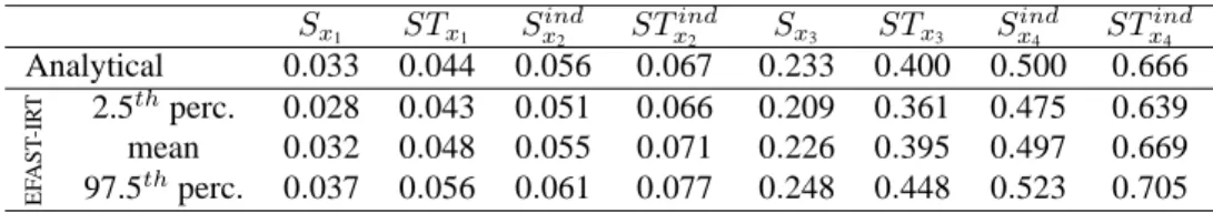
the desired constraints. The sample fills the input space quite well. Tab. 1 shows good agreement between the mean 227
estimates of the sensitivity indices and the analytical values. The results indicate that(x3, x4) are the most relevant
228
inputs for the response variance. 229
By referring to the work of [1], it can be inferred that one possible ANOVA decomposition (in the Sobol’ sense 230
[5]) off (x) is:
231
f (x) = f0+ f1(x1) + f¯2(¯x2) + f1¯2(x1, ¯x2) + f3(x3) + f¯4(¯x4) + f3¯4(x3, ¯x4) (26)
where the functions in Eq. (26) have the same properties than those of the Sobol’s ANOVA decomposition [5]. In 232
particular, they are orthogonal. This property of orthogonality allows to cast the variance off (x), denoted V , as
233
follows: 234
V = V1+ V2ind+ V12+ V3+ V4ind+ V34 (27)
withVi= E[fi2(xi)], Viind= E[f¯i2(¯xi)] and Vij = E[fij2(xi, ¯xj)]. By denoting V Ti= Vi+ Vijyields the following 235
variance decomposition, 236
Vy= V T1+ V2ind+ V T3+ V4ind. (28)
The normalization of the latter equation byV yields the following relationship between the variance-based sensitivity
indices, STx1+ S ind x2 + STx3+ S ind x4 = 1.
The analytical variance-based sensitivity indices reported in Tab. 1 satisfy this relationship. Moreover, we can infer 237
thatSTx1+ S
ind
x2 = 0.10, which indicates that the pair (x1, x2) explains 10% of the response variance since the pairs
238
(x1, x2) and (x3, x4) are independent.
239
TABLE 1: One hundred replicate estimates of the sensitivity indices computed with EFAST-IRT.
Sx1 STx1 Sindx2 ST ind x2 Sx3 STx3 Sxind4 ST ind x4 Analytical 0.033 0.044 0.056 0.067 0.233 0.400 0.500 0.666 E F A S T -I R T 2.5thperc. 0.028 0.043 0.051 0.066 0.209 0.361 0.475 0.639 mean 0.032 0.048 0.055 0.071 0.226 0.395 0.497 0.669 97.5thperc. 0.037 0.056 0.061 0.077 0.248 0.448 0.523 0.705
6.2 The Ishigami function with EFAST-INT
240
The Ishigami function is one of the benchmarks model for assessing the efficiency of GSA methods [39]. It has been 241
intensively used by statisticians to test their sensitivity analysis approaches in the case of independent inputs (e.g. 242
[40,41], among others). Recently, the authors in [21] introduced a new method for computingSxiandST
ind xi in the
243
case of models with correlated inputs and tested it on the Ishigami function. We repeat here the same example with 244
0 0.1 0.2 0.3 0.4 0.5 0.6 0.7 0.8 0.9 1 0 0.1 0.2 0.3 0.4 0.5 0.6 0.7 0.8 0.9 1
x
1x
2x
3x
4FIG. 1: Some draws obtained with FAST after the inverse Rosenblatt transformation. We have x1+ x2 ≤1 (blue circles) and x3+ x4≥1 (red stars).
EFAST-INT but compute(Sxi, STxindi , S
ind
xi , STxi), ∀i = 1, 2, 3. The Ishigami function writes,
245
f (x) = sin x1+ 7 sin2x2+ 0.1x43sin x1 (29)
with input variables being uniformly distributed:−π ≤ xi≤ π, i = 1, 2, 3. Note that this function is non-linear in all 246
inputs andx2does not interact with the other two variables. Although this function has a low dimension (three inputs
247
only), it is a challenging function for EFAST because the last term, which represents the interaction betweenx1and
248
x3, is strongly non-linear and its Fourier coefficients have considerable amplitudes at high frequencies. This strong
249
non-linearity led us to choose a considerably high value ofM . The difficulty of the test was emphasized because a
250
correlationr13∈] − 1, 1[ was imposed between x1andx3.
251
Likewise the previous exercise, 100 replication estimates of the sensitivity indices were performed. The design 252
of the EFAST-INT was the following:M = 15, N = 8 191, ω∼i= (5, 8) and ωi = 273. We chose higher N here 253
than in the previous example because of the strong non-linearities mentioned above. Following the work of [21], the 254
exercise was conducted by varying the correlation coefficientr13within] − 1, 1[.
255
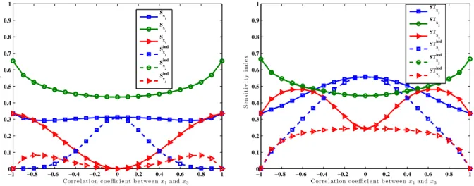
The results are depicted in Fig. 2. To our best knowledge, no analytical sensitivity indices are available for this 256
test function. We can infer that, becausex2is not correlated to the other two inputs, its full and independent sensitivity
257
indices are equal. Besides, becausex2does not interact with the other two inputs, its total and first-order indices are
258
also equal. Moreover, we note that the full indexSxiis always greater or equal to the independent indexS
ind xi (resp.
259
STxi ≥ STxindi ). However, we may also findS
ind
xi > Sxi (orSTxindi > STxi) as also shown in the previous exercise
260
(see Tab. 1). 261
As far asx1andx3are concerned we note that, when the correlation coefficient is zero, as expected the full and
262
independent sensitivity indices are equal. Whenr13is close to±1, the independent sensitivity indices (both first and
263
total order) ofx1andx3are null. This makes sense because ifr13 = ±1, then all the information in f(x) is captured
264
by only one of the pairs(x1, x2) or (x2, x3). Indeed, in this case, x1andx3contain the same information and it is
265
not possible to distinguish their individual contributions in the model response. This finding is peculiarly important 266
for the modeller as it indicates that the output uncertainty is explained by one of these two pairs only, thus, allowing 267
some kind of dimensionality reduction. Indeed, the modeller now knows that to obtain narrower output uncertainty, 268
he/she should pay some further effort to reduce the uncertainty either in the pair(x1, x2) or in (x2, x3).
269 −1 −0.8 −0.6 −0.4 −0.2 0 0.2 0.4 0.6 0.8 1 0 0.1 0.2 0.3 0.4 0.5 0.6 0.7 0.8 0.9 1
Corre l ati on c o e ffic i e nt b e twe e n x1and x3
S e n s it iv it y in d e x Sx 1 Sx 2 Sx 3 Sx 1 ind Sx 2 ind Sx 3 ind −1 −0.8 −0.6 −0.4 −0.2 0 0.2 0.4 0.6 0.8 1 0 0.1 0.2 0.3 0.4 0.5 0.6 0.7 0.8 0.9 1
Corre l ati on c o e ffic i e nt b e twe e n x1and x3
S e n s it iv it y in d e x STx 1 STx 2 STx 3 STindx 1 STind x 2 STind x 3
7. CONCLUSION
270
Performing global sensitivity analysis of model output with dependent inputs is a challenging issue. Variance-based 271
sensitivity indices have been defined in [1,19,21] and different approaches have been proposed to estimate them. Four 272
types of sensitivity indices can be of interest: (i) the full first-order (resp. full total) sensitivity index that measures 273
the amount of model response variance explained by an input factor which takes into account its dependence with the 274
other inputs; (ii) the full total-order sensitivity index that measures the amount of model response variance explained 275
by an input factor which takes into account the both its dependence and interactions with the other inputs; (iii) 276
the independent first-order sensitivity index of an input that measures its relative contribution alone to the response 277
variance by ignoring its dependence with the other inputs; and finally (iv) the independent total-order sensitivity index 278
of an input that measures its relative contribution to the response variance by ignoring its dependence with the other 279
input variables but by accounting for its interactions with the latter. 280
The Fourier amplitude sensitivity test is one of the first methods for variance-based global sensitivity analysis 281
[10]. Since that, the method has been extended by several authors [11,29,30,37,38]. Specifically, in [30] FAST has 282
been adapted to account for correlations among inputs by using the sampling technique of Iman and Conover [24]. 283
In this work, we extend FAST to compute the four sensitivity indices defined above. The main idea of our approach 284
is to impose either a dependence structure amongst the inputs with the inverse Rosenblatt transformation [22], with 285
Algorithm 2 denoted EFAST-IRT, or a correlation structure with the inverse Nataf transformation [23], denoted 286
EFAST-INT (see Algorithm 3). The numerical tests shown in the paper confirm the suitability of both EFAST-IRT 287
and EFAST-INT. 288
The sampling strategy proposed by [21] allows for estimating the overall full first-order sensitivity indices and 289
the independent total sensitivity indices with(2n+2) (quasi) Monte Carlo samples. The sampling strategies proposed
290
in [1] allows for assessing the four sensitivity indices of all the input variables with 4n (quasi) Monte Carlo samples.
291
In the present work, we show that 2n samples are sufficient to compute the four sensitivity indices of all the inputs
292
with either EFAST-IRT or EFAST-INT. 293
ACKNOWLEDGMENTS
294
The corresponding author would like to thank the French National Research Agency for its financial support (Research 295
project RESAIN n◦ANR-12-BS06-0010-02). 296
REFERENCES
297
1. Mara, T.A., Tarantola, S., and Annoni, P., Non-parametric methods for global sensitivity analysis of model output with
298
dependent inputs, Environmental Modelling and Software, 72:173–183, 2015.
299
2. Blatman, G. and Sudret, B., Adaptive sparse polynomial chaos expansion based on least angle regression, Journal of
Compu-300
tational Physics, 230(6):2345–2367, 2011.
301
3. Anstett-Collin, F., Goffart, J., Mara, T., and Denis-Vidal, L., Sensitivity analysis of complex models: Coping with dynamic
302
and static inputs, Reliability Engineering and System Safety, 134:268–275, 2015.
303
4. Saltelli, A., Ratto, M., Andres, T., Campolongo, F., Cariboni, J., Gatelli, D., Saisana, M., and Tarantola, S., Global Sensitivity
304
Analysis: The Primer, Probability and Statistics, John Wiley and Sons, Chichester, 2008.
305
5. Sobol’, I.M., Sensitivity estimates for nonlinear mathematical models, Math. Mod. and Comput. Exp., 1:407–414, 1993.
306
6. Chun, M.H., Han, S.J., and Tak, N.I., An uncertainty importance measure using distance metric for the change in a cumulative
307
distribution function, Reliability Engineering and System Safety, 70:313–321, 2000.
308
7. Borgonovo, E., Measuring uncertainty importance: Investigation and comparison of alternative approaches, Risk Analysis,
309
26(5):1349–1361, 2006.
310
8. Sobol’, I.M., Global sensitivity indices for nonlinear mathematical models and their monte carlo estimates, Mathematics and
311
Computers in Simulation, 55:271–280, 2001.
312
9. Saltelli, A., Making best use of model evaluations to compute sensitivity indices, Computational Physics Communications,
313
145:280–297, 2002.
314
10. Cukier, R.I., Fortuin, C.M., Shuler, K.E., Petschek, A.G., and Schaibly, J.H., Study of the sensitivity of coupled reaction
315
systems to uncertainties in rate coefficients. I. theory, J. Chemical Physics, 59:3873–3878, 1973.
316
11. Saltelli, A., Tarantola, S., and Chan, K., A quantitative model independent method for global sensitivity analysis of model
317
output, Technometrics, 41:39–56, 1999.
318
12. Oakley, J.E. and O’Hagan, A., Probabilistic sensitivity analysis of complex models: a Bayesian approach, J. Royal Statist.
319
Soc. B, 66:751–769, 2004.
320
13. Ratto, M., Pagano, A., and Young, P., State dependent parameter metamodelling and sensitivity analysis, Computer Physics
321
Communications, 117(11):863–876, 2007.
322
14. Pearson, K. On the general theory of skew correlation and non-linear regression. In Mathematical contributions to the theory
323
of evolution, Vol. XIV. Drapers’s Company Research Memoirs, 1905.
324
15. McKay, M.D., Variance-based methods for assessing uncertainty importance, Tech. Rep., Technical Report
NUREG-325
1150,UR-1996-2695, Los Alamos National Laboratory, 1996.
16. Homma, T. and Saltelli, A., Importance measures in global sensitivity analysis of nonlinear models, Reliability Engineering
327
and System Safety, 52:1–17, 1996.
328
17. Saltelli, A. and Tarantola, S., On the relative importance of input factors in mathematical models: Safety assessment for
329
nuclear waste disposal, Journal of the American Statistical Association, 97:702–709, 2002.
330
18. Xu, C. and Gertner, G.Z., Uncertainty and sensitivity analysis for models with correlated parameters, Reliability Engineering
331
and System Safety, 93:1563–1573, 2008b.
332
19. Mara, T.A. and Tarantola, S., Variance-based sensitivity indices for models with dependent inputs, Reliability Engineering
333
and System Safety, 107:115–121, 2012.
334
20. Zhou, C., Lu, Z., Zhang, L., and Hu, J., Moment independent sensitivity analysis with correlations, Applied Mathematical
335
Modelling, 38:4885–4896, 2014.
336
21. Kucherenko, S., Tarantola, S., and Annoni, P., Estimation of global sensitivity indices for models with dependent variables,
337
Computer Physics Communications, 183:937–946, 2012.
338
22. Rosenblatt, M., Remarks on the multivariate transformation, Annals of Mathematics and Statistics, 43:470–472, 1952.
339
23. Nataf, A., D´etermination des distributions dont les marges sont donn´ees, Comptes Rendus de l’Acad´emie des Sciences,
340
225:42–43, 1962.
341
24. Iman, R.I. and Conover, W.J., A distribution-free approach to inducing rank correlation among input variables,
Communica-342
tions in Statistics: Simulation and Computation, 11:311–334, 1982.
343
25. Li, G., Rabitz, H., Yelvington, P.E., Oluwole, O.O., Bacon, F., Kolb, C.E., and Schoendorf, J., Global sensitivity analysis for
344
systems with independent and/or correlated inputs, J. Physical Chemistry, 114:6022–6032, 2010.
345
26. Caniou, Y., Analyse de sensibilit´e globale pour les mod`eles imbriqu´es et multi´echelles, PhD thesis, University Blaise Pascal,
346
Clermont-Ferrand, 2012.
347
27. Chastaing, G., Gamboa, F., and Prieur, C., Generalized Hoeffding-Sobol decomposition for dependent variables – application
348
to sensitivity analysis, Electronic Journal of Statistics, 6:2420–2448, 2012.
349
28. Da Veiga, S., Wahl, F., and Gamboa, F., Local polynomial estimation for sensitvity analysis of models with correlated inputs,
350
Technometrics, 51(4):452–463, 2009.
351
29. Xu, C., Decoupling correlated and uncorrelated uncertainty contributions for nonlinear models, Applied Mathematical
Mod-352
elling, 37:9950–9969, 2013.
353
30. Xu, C. and Gertner, G.Z., A general first-order global sensitivity analysis method, Reliability Engineering and System Safety,
354
93:1060–1071, 2008a.
355
31. Fisher, R.A., The distribution of the partial correlation coefficient, Metron, pp. 329–332, 1924.
32. Sobol’, I.M., Turchaninov, V.I., Levitan, Y.L., and Shukman, B.V. Quasi-random sequence generator (routine LPTAU51).
357
Keldysh Institute of Applied Mathematics, Russian Academy of Sciences, 1992.
358
33. Li, H., Lu, Z., and Yuan, X., Nataf transformation based point estimate method, Chinese Science Bulletin, 53(17):2586–2592,
359
2008.
360
34. Ditlevsen, O. and Madsen, H.O., Structural Reliability Methods, John Wiley and Sons, New York, 1996.
361
35. Cukier, R.I., Schaibly, J.H., and Shuler, K.E., Study of the sensitivity of coupled reaction systems to uncertainties in rate
362
coefficients. iii. analysis of the approximations, J. Chemical Physics, 63:1140–1149, 1975.
363
36. Satterthwaite, F.E., Random balance experimentation, Technometrics, 1:111–137, 1959.
364
37. Tarantola, S., Gatelli, D., and Mara, T.A., Random balance designs for the estimation of first-order global sensitivity indices,
365
Reliability Engineering and System Safety, 91:717–727, 2006.
366
38. Mara, T.A., Extension of the rbd-fast method to the computation of global sensitivity indices, Reliability Engineering and
367
System Safety, 94:1274–1281, 2009.
368
39. Saltelli, A., Chan, K., and Scott, E.M., Sensitivity analysis, John Wiley and Sons, Chichester, 2000.
369
40. Sudret, B., Global sensitivity analysis using polynomial chaos expansions, Reliability Engineering and System Safety, 93:964–
370
979, 2008.
371
41. Marrel, A., Iooss, B., Laurent, B., and Roustant, O., Calculations of Sobol indices for the Gaussian process metamodel,
372
Reliability Engineering and System Safety, 94:742–751, 2009.