Alternative Asymptotics and the Partially Linear
Model with Many Regressors
Matias D. Cattaneo
yMichael Jansson
zWhitney K. Newey
xJuly 9, 2015
Abstract
Many empirical studies estimate the structural e¤ect of some variable on an out-come of interest while allowing for many covariates. We present inference methods that account for many covariates. The methods are based on asymptotics where the number of covariates grows as fast as the sample size. We …nd a limiting normal dis-tribution with variance that is larger than the standard one. We also …nd that with homoskedasticity this larger variance can be accounted for by using degrees of freedom adjusted standard errors. We link this asymptotic theory to previous results for many instruments and for small bandwidths distributional approximations.
JEL classi…cation: C13, C31.
Keywords: non-standard asymptotics, partially linear model, many terms, adjusted variance.
The authors are grateful for comments from Xiaohong Chen, Victor Chernozhukov, Alfonso Flores-Lagunes, Lutz Kilian, seminar participants at Bristol, Brown, Cambridge, Exeter, Indiana, LSE, Michigan, MSU, NYU, Princeton, Rutgers, Stanford, UCL, UCLA, UCSD, UC-Irvine, USC, Warwick and Yale, and conference participants at the 2010 Joint Statistical Meetings and the 2010 LACEA Impact Evaluation Network Conference. We also thank the Editor and two reviewers for their comments. The …rst author gratefully acknowledges …nancial support from the National Science Foundation (SES 1122994 and SES 1459931). The second author gratefully acknowledges …nancial support from the National Science Foundation (SES 1124174 and SES 1459967) and the research support of CREATES (funded by the Danish National Research Foundation under grant no. DNRF78). The third author gratefully acknowledges …nancial support from the National Science Foundation (SES 1132399).
yDepartment of Economics, University of Michigan. zDepartment of Economics, UC Berkeley and CREATES. xDepartment of Economics, MIT.
1
Introduction
Many empirical studies estimate the structural, causal, or treatment e¤ect of some variable on an outcome of interest. For example, we might be interested in estimating the e¤ect of some government policy on an outcome such as income. Since policies and many other variables are not exogenous, researchers rely on a variety of approaches based on observational data when trying to estimate such e¤ects. One important method is based on assuming that the variable of interest can be taken as exogenous after controlling for a su¢ cient set of other factors or covariates. See, for example, Heckman and Vytlacil(2007) and Imbens and Wooldridge (2009) for recent reviews and further references.
A problem empirical researchers face when relying on covariates to estimate a structural e¤ect is the availability of many potential controls. Typically, intuition will suggest a set of variables that might be important but will not identify exactly which variables are im-portant or the functional form with which variables should enter the model. This lack of clear guidance about what variables to use leaves researchers with a potentially vast set of potential covariates including raw regressors available in the data as well as interactions and other nonlinear transformations thereof. Many economic studies include very many of these variables in order to control for as broad array of covariates as possible. For example, it is common to include dummy variables for many potentially overlapping groups based on age, cohort, geographic location, etc. Even when some controls are dropped after valid covariate selection, as was developed by Belloni, Chernozhukov, and Hansen (2014), many controls may remain in the …nal regression speci…cation.
We present inference methods that account for the presence of many controls in regression models. We do this using a large sample approximation where the number of covariates grows as fast as the sample size. We …nd a limiting normal distribution with variance that is larger than the standard asymptotic variance. We show that with homoskedasticity this larger variance is fully accounted for by using standard errors with a degrees of freedom adjustment for inclusion of many covariates. This asymptotics and the associated standard errors provides an important justi…cation for the practice of adjusting for degrees of freedom even when disturbances are not normally distributed. As always the asymptotics is meant as an approximation that provides useful inference methods for applications. In this way the asymptotic approximation given here should prove useful in practice.
This paper also adds to the literature on regression where the number of regressors grow with the sample size. Huber (1973) showed that …tted regression values are not asymptot-ically normal when the number of regressors grows as fast as sample size. The problem is
covariates gets large. Recently, El Karoui, Bean, Bickel, Lim, and Yu (2013) showed that, with a Gaussian distributional assumption on the regressors, certain coe¢ cients and con-trasts are asymptotically normal when the number of regressors grow as fast as sample size, but do not give inference results. We do give inference results in showing that the degrees of freedom adjustment to standard errors accounts correctly for many covariates and do not impose distributional assumptions on the regressors. We also use a di¤erent and simpler ap-proach to the asymptotic theory. We note that our results were presented at the 2010 Joint Statistical Meetings and are independent of El Karoui, Bean, Bickel, Lim, and Yu (2013).
The asymptotics here is based on asymptotic normality results for degenerate U-statistics. To help explain and motivate this theory we note that asymptotic normality for degenerate U-statistics has already been used in other settings. Such results are the basis for the many instrument asymptotics where the number of instruments grows as fast as the sample size.
Kunitomo(1980) andMorimune(1983) derived asymptotic variances that are larger than the usual formulae when the number of instruments and sample size grow at the same rate, and
Bekker (1994) and others provided consistent estimators of these larger variances. Hansen, Hausman, and Newey(2008) showed that using many instrument standard errors provides a improvement for a range of number of instruments. This asymptotics has also proven useful for small bandwidth approximations for kernel-based density-weighted average derivative estimators in Cattaneo, Crump, and Jansson (2010, 2014b). They show that when the bandwidth shrinks faster than needed for consistency of the kernel estimator, the variance of the estimator is larger than the usual formula. They also …nd that correcting the variance provides an improvement over standard asymptotics for a range of bandwidths.
We use a common framework for these results to motivate the asymptotic theory. The common framework is that the object determining the limiting distribution is a V-statistic, which can be decomposed into a bias term, a sample average, and a “remainder” that is an asymptotically normal degenerate U-statistic. Asymptotic normality of the remainder distinguishes this setting from others with degenerate U-statistic. Here asymptotic normality occurs because the number of covariates goes to in…nity, while the behavior of a degenerate U-statistic is di¤erent in other settings. When the number of covariates grows as fast as the sample size the remainder has the same magnitude as the leading term, resulting in an asymptotic variance larger than just the variance of the leading term. The many covariate, many instrument, and small bandwidth results share this structure. In keeping with this common structure, we refer here to such results under the general heading of “alternative asymptotics”. While not all semiparametric estimation problems share this structure, we show by example that its scope may indeed be useful for econometrics. In the conclusions section below we also discuss its limitations and its relation to other type of alternative
asymptotic approximations in semiparametrics problems and other loosely related contexts. An important generalization to the results presented herein is to asymptotics and infer-ence with many covariates under heteroskedasticity. Constructing consistent standard errors estimator under heteroskedasticity of unknown form in this setting turns out to be quite challenging. In Cattaneo, Jansson, and Newey (2015), we present a detailed discussion of heteroskedasticity-robust standard errors for linear models where the number of covariates increases at the same rate as the sample size, which covers the partially linear model with number terms growing at the same rate as the sample size.
The rest of the paper is organized as follows. Section2describes the common structure of many instrument and small bandwidth asymptotics, and also shows how the structure leads to new results for the partially linear model. Section 3 formalizes the new distributional approximation for many covariates. Section4 reports results from a small simulation study aimed to illustrate our results in small samples. Section 5 concludes. Appendix A collects the proofs of our results, while Appendix B discusses heuristically how our results can be extended to the case of generated regressors and related problems.
2
A Common Structure
We consider inference on structural e¤ects in an environment where variables of interest may be taken as exogenous conditional on covariates. We pose the problem in the framework of a partially linear model. Let (yi; x0i; zi0)0, i = 1; : : : ; n, be a random sample satisfying
yi = x0i 0+ g(zi) + "i; E["ijxi; zi] = 0; (1)
where yiis a scalar dependent variable, xi 2 Rdare the treatment/policy variables of interest,
zi are explanatory variables, g(z) is an unknown function, and E[V[xijzi]]is of full rank. The
goal of the analysis is to conduct inference about the structural e¤ect 0.
A series estimator of 0 is obtained by regressing yi on xi and functions of zi. To describe
the estimator, let p1(z); p2(z); : : :be approximating functions, such as polynomials or splines,
and let pK(z) = (p1(z); : : : ; pK(z))0 be a K-dimensional vector of such functions. We consider
a regression that includes a K 1 vector of covariates pK(zi) that may consist of zi and
transformations of zi to adequately approximate g(zi). The conditional mean restriction
E["ijxi; zi] = 0 means that xi may be considered exogenous after controlling linearly for
variables that can approximate g(zi): We will assume that linear combinations of these
M = In PK(PK0 PK) 1PK0 ; where PK = [pK(z1); : : : ; pK(zn)]0. A series estimator of 0 in (1) is given by ^ = n X i=1 n X j=1 Mijxix0j ! 1 n X i=1 n X j=1 Mijxiyj ! :
Donald and Newey (1994) gave conditions for asymptotic normality of this estimator using standard asymptotics. See also Linton (1995) and references therein for related asymptotic results when using kernel estimators.
Conditional on Z = [z1; : : : ; zn]0, ^ depends on a V-statistic. Plugging in for yi for each
i and solving gives
p n(^ 0) = ^n1Sn; (2) with ^ n= 1 n n X i=1 n X j=1 Mijxix0j; Sn = 1 p n n X i=1 n X j=1 xiMij(gj + "j);
where gi = g(zi):Conditional on Z, the term Sn is a V-statistic
Sn = n X i=1 n X j=1 unij(Wi; Wj);
where Wi = (x0i; "i)0 and unij(Wi; Wj) = xiMij(gj + "j)=pn. We assume throughout this
section that there exists a sequence of non-random matrices n satisfying n1^n !p Id for
Id the d d identity matrix, and hence we focus on the V-statistic Sn. (All limits are taken
as n ! 1 unless explicitly stated otherwise.)
To explain the many covariate asymptotics, and to provide a link to previous work on many instruments and small bandwidths, it is helpful to provide a general analysis of the V-statistic Sn. This V-statistic has a well known (Hoe¤ding-type) decomposition that we
describe here because it is an essential feature of the common structure. For notational implicitly we will drop the Wi and Wj arguments and set unij = unij(Wi; Wj) and ~unij =
un
ij + unji E[unij + unji]. Let k k denote the Euclidean norm. If E[kunijk] < 1 for all i; j; n,
then Sn = Bn+ n+ Un; (3) where Bn= E[Sn]; n = n X i=1 n i(Wi); Un= n X i=2 Dni(Wi; :::; W1); n i(Wi) = unii E[u n ii] + n X j=1;j6=i E[~unijjWi];
Dni(Wi; :::; W1) = n
X
j=1;j<i
(~unij E[~unijjWi] E[~unijjWj]):
It is straightforward to see that E[ ni(Wi)] = 0, E[Din(Wi; :::; W1)jWi 1; :::; W1] = 0, and
E[ nUn] = 0. This decomposition of a V-statistic is well known (e.g., van der Vaart(1998,
Chapter 11)), and shows that Sn can be decomposed into a sum nof independent terms, a
U-statistic remainder Un that is a martingale di¤erence sum and uncorrelated with n, and
a pure bias term Bn.1 The decomposition is important in many of the proofs of asymptotic
normality of semiparametric estimators, including Powell, Stock, and Stoker (1989), with the limiting distribution being determined by n, and Un being treated as a “remainder”
that is of smaller order under a particular restriction on the tuning parameter sequence (e.g., when the number of covariates increase slowly enough).
An interesting property of Un is that it is asymptotically normal at some rate when the
number of covariates grow. To be speci…c, if regularity conditions speci…ed below hold and K ! 1 with the sample size, it turns out that
2 4 V[ n] 1=2 n V[Un] 1=2Un 3 5 !dN (0; I2d):
In other settings, where the underlying kernel of the U-statistic does not vary with the sample size, the asymptotic behavior of Un can be di¤erent. Many degenerate U-statistics
will converge to a weighted sum of independent chi-square random variables (e.g., van der Vaart (1998, Chapter 12)). However, as the number of covariates grows, the kernel of the underlying U-statistic forming Un changes with the sample in such a way that the individual
contributions Dn
i(Wi; :::; W1) to Un are small enough to satisfy a Lindeberg-Feller condition
leading to a Gaussian limiting distribution (usually established using the martingale property of Un). For an interesting discussion of this phenomenon, see de Jong (1987). This type of
asymptotic normality result for degenerate U-statistics has previously been shown in other settings, as further explained below.
When the number of covariates grows as fast as the sample size V[ n] and V[Un] have
the same magnitude in the limit. Because of uncorrelatedness of nand Un, the asymptotic
variance will be larger than the usual formula which is limn!1V[ n] (assuming the limit
exists). As a consequence, consistent variance estimation under many covariate asymptotics requires accounting for the contribution of Un to the (asymptotic) sampling variability of
1In time series contexts, the exact decomposition is less useful, but approximations thereof with properties
the statistic.
To apply this calculation to many covariates, note that by E["ijxi; zi] = 0 we have
E[xi"ijZ] = 0. Therefore, letting unij = unij(Wi; Wj) as we have done previously, we have
E[unijjZ] = hiMijgj=pn; unij E[u n ijjZ] = Mij(vigj+ xi"j) =pn; ~ unij = Mij(vjgi+ vigj+ xj"i+ xi"j) = p n; E[~unijjWi; Z] = Mij(vigj+ hj"i) = p n; for i 6= j, where hi = h(zi) = E[xijzi]and vi = xi hi. In this case, the bias term in (3) is
Bn = 1 p n n X i=1 n X j=1 Mijhigj;
which will be negligible under regularity conditions, as shown in the next section. Moreover,
n= 1 p n n X i=1 Miivi"i+ Rn; Rn= 1 p n n X i=1 n X j=1 Mij(vigj + hi"j);
where Rn has mean zero and converges to zero in mean square as K grows, as further
discussed below. Under standard asymptotics Mii will go to one and hence the limiting
variance of the leading term in n corresponds to the usual asymptotic variance. Finally,
we …nd that the degenerate U-statistic term is
Un = 1 p n n X i=1 n X j=1;j<i Mij(vi"j + vj"i) = 1 p n n X i=1 n X j=1;j<i Qij(vi"j + vj"i) ;
where Qij is the (i; j)-th component of PK(PK0 PK) 1PK0 . Remarkably, as discussed below,
this term is essentially the same as the degenerate U-statistic term for certain instrumental variables estimators. Consequently, a central limit theorem of Chao, Swanson, Hausman, Newey, and Woutersen(2012) that was applied to many instrument asympotics is applicable to regression with many covariates. We will employ it to show that Un is asymptotically
normal as K ! 1.
Distribution theory with many covariates may be seen as a generalization of the conven-tional asymptotics in the sense that under convenconven-tional asymptotics the asymptotic variances emerging from both approaches coincide. But, the alternative asymptotic approximation also allows for the covariates to grow at the same rate as the sample size, where the limiting as-ymptotic variance is larger. Thus, in general, there is no reason to expect that the usual standard error formulas derived under conventional asymptotics will remain valid more gen-erally. From this perspective, many covariate asymptotics provides theoretical justi…cation
for new standard error formulas that are consistent under both conventional and many co-variate asymptotics. We refer to the latter standard error formulas as being more robust than the usual standard error formulas available in the literature. For instance, using these ideas, more robust standard errors formulas were derived previously for many instrument asymptotics in IV models (Hansen, Hausman, and Newey (2008)) and small bandwidth asymptotics in kernel-based semiparametrics (Cattaneo, Crump, and Jansson(2014b)).
Accounting for the presence of Un should also yield improvements when numbers of
co-variates do not satisfy the knife-edge condition of growing at the same rate as the sample size. For instance, if the number of covariates grows just slightly slower than the sample size then accounting for the presence of Un should still give a better large sample
approxima-tion. Hansen, Hausman, and Newey(2008) show such an improvement for many instrument asymptotics. It would be good to consider such improved approximations more generally, though it is beyond the scope of this paper to do so.
To motivate and provide background for this approach we show next that both many in-strument asymptotics and small bandwidth asymptotics have the structure described above.
2.1
Connection with Many Instrument Asymptotics
To link many covariate asymptotics with many instrument asymptotics we focus on the JIVE2 estimator of Angrist, Imbens, and Krueger (1999), but the idea applies to other IV estimators such as the limited information maximum likelihood estimator. See Chao, Swanson, Hausman, Newey, and Woutersen (2012) for more details, including regularity conditions under which the following discussion can be made rigorous.
Let (yi; x0i; zi0)0, i = 1; : : : ; n, be a random sample generated by the model
yi = x0i 0+ "i; E["ijzi] = 0; (4)
where yi is a scalar dependent variable, xi 2 Rd is a vector of endogenous variables, "i is a
disturbance, and zi 2 RK is a vector of instrumental variables.
To describe the JIVE2 estimator of 0 in (4), now let Qij denote the (i; j)-th element of
Q = Z(Z0Z) 1Z0, where Z = [z
1; ; zn]0. After centering and scaling, the JIVE2 estimator
^ satis…es p n(^ 0) = 1 n n X i=1 n X j=1;j6=i Qijxix0j ! 1 1 p n n X i=1 n X j=1;j6=i Qijxi"j ! :
Conditional on Z; ^ has the structure in (2) with Wi = (x0i; "i)0 and ^n = 1 n n X i=1 n X j=1;j6=i Qijxix0j; u n ij(Wi; Wj) = 1(i6= j)Qijxi"j= p n;
where 1( ) is the indicator function. For i 6= j, E[unij(Wi; Wj)jZ] = 0 and
E[unij(Wi; Wj)jWi; Z] = QijxiE["jjZ] = 0; E[unji(Wj; Wi)jWi; Z] = Qij j"i=
p n;
where i = E[xijzi] can be interpreted as the reduced form for observation i. As a
conse-quence, (3) is satis…ed with Bn= 0, n i(Wi) = ( n X j=1;j6=i Qij j)"i = i(1 Qii)"i= p n ( i n X j=1 Qij j)"i= p n; Din(Wi; :::; W1) = n X j=1;j<i Qij(vi"j + vj"i) = p n; vi = xi i: Because i Pn
j=1Qij j is the i-th residual from regressing the reduced form observations
on Z, by appropriate de…nition of the reduced form this can generally be assumed to vanish as the sample size grows. In that case,
n = 1 p n n X i=1 i(1 Qii)"i+ op(1):
Furthermore, under standard asymptotics Qiiwill go to zero, so the limiting variance of the
leading term in n corresponds to the usual asymptotic variance for IV. The degenerate
U-statistic term is Un = 1 p n n X i=1 n X j=1;j<i Qij(vi"j + vj"i) :
Chao, Swanson, Hausman, Newey, and Woutersen (2012) apply a martingale central limit theorem to show that this Un will be asymptotically normal when K ! 1 and certain
regularity conditions hold. Here we see that the Un term for JIVE2 has the same form as
for many covariates. Thus, many covariate asymptotics can be obtained by using previous results for many instruments.
2.2
Connection with Small Bandwidth Asymptotics
We can also show that small bandwidth asymptotics for certain kernel-based semiparametric estimators is based on a generate U-statistic like that considered above. To keep the expo-sition simple we focus on an estimator of the integrated squared density, but the structure of this estimator is shared by the density-weighted average derivative estimator of Powell, Stock, and Stoker (1989) treated in Cattaneo, Crump, and Jansson(2014b) and more gen-erally by estimators of density-weighted averages and ratios thereof (see, e.g.,Newey, Hsieh, and Robins (2004, Section 2) and references therein). Furthermore, these ideas are also ap-plicable to other semiparametric problems such as those involving (i ) certain functionals of U-processes arising in latent models as in Aradillas-Lopéz, Honoré, and Powell (2007) and references therein, (ii ) U-statistics used for speci…cation testing as in Li and Racine (2007, Chapter 12) and references therein, and (iii ) U-statistics obtained from convolution estima-tors as inSchick and Wefelmeyer(2013) and references therein. Since the main purpose here is to highlight the connections between many covariate asymptotics and other alternative asymptotics in the literature, rather than to extend the scope of alternative asymptotics, we do not discuss those other potential applications here.
Suppose xi, i = 1; : : : ; n, are i.i.d. continuously distributed p-dimensional random vectors
with smooth p.d.f. f0 and consider estimation of the integrated squared density
0 =
Z
Rp
f0(x)2dx = E[f0(xi)]:
A leave-one-out kernel-based estimator is
^ = 1 n(n 1) n X i=1 n X j=1;j6=i Kh(xi xj);
where K(u) is a symmetric kernel and Kh(u) = h pK(u=h). As shown by Giné and Nickl
(2008), this estimator is optimal, attaining root-n consistency under weak conditions. This estimator has the V-statistic form of (2) with Wi = xi and
^ n= 1; unij(Wi; Wj) = 1 p n(n 1)1(i6= j)fKh(xi xj) 0g: Let fh(x) = R
RpK(u)f0(x + hu)du and h =
R Rpfh(x)f0(x)dx. By symmetry of K(u), E[unij(Wi; Wj)jWi] = E[unji(Wj; Wi)jWi] = 1 p n(n 1)ffh(xi) 0g;
E[unij(Wi; Wj)] =
1 p
n(n 1)f h 0g; so the terms in the decomposition (3) are of the form
Bn= p nf h 0g; n= 1 p n n X i=1 2ffh(xi) hg; Un= 2 p n(n 1) n X i=1 n X j=1;j<i fKh(xi xj) fh(xi) fh(xj) + hg:
Here, 2ffh(xi) hg is an approximation to the well known in‡uence function 2ff0(xi) 0g for estimators of the integrated squared density. Under regularity conditions, fh(xi)
converges to f0(xi)in mean square as h ! 0, so that
n = 1 p n X 1 i n 2ff0(xi) 0g + op(1):
A martingale central limit theorem can be applied as in Cattaneo, Crump, and Jansson
(2014b) to show that the degenerate U-statistic term Un will be asymptotically normal as
h ! 0 and n ! 1, provided that n2hp ! 1. It is easy to show that n2hpV[Un] ! = 0
R
RpK(u)
2du, under mild regularity conditions. Alternative asymptotics occurs when hp
shrinks as fast as 1=n, resulting in V[ n] and V[Un]having the same magnitude in the limit.
3
Many Covariate Asymptotics
In this section we make precise the previous discussion for many covariate asymptotics and also consider inference under homoskedasticity. The estimator ^ described above for many covariates can be interpreted as a two-step semiparametric estimator with tuning parameter K, the …rst step involving series estimation of the unknown (regression) functions g(z) and h(z). Donald and Newey (1994) gave conditions for asymptotic normality of this estimator when K=n ! 0. Here we generalize their …ndings by obtaining an asymptotic distributional result that is valid even when K=n is bounded away from zero.
The analysis proceeds under the following assumption.
Assumption PLM (Partially Linear Model) (a) (yi; x0i; zi0)0, i = 1; : : : ; n, is a random sample.
(b) There is a C < 1 such that E["4
(c) There is a C > 0 such that E["2ijxi; zi] C and min(E[viv0ijzi]) C.
(d) rank(PK) = K (a.s.) and there is a C > 0 such that Mii C.
(e) For some g; h > 0, there is a C < 1 such that
min
g2RK
E[jg(zi) 0gpK(zi)j2] CK 2 g; min h2RK d
E[kh(zi) 0hpK(zi)k2] CK 2 h:
Because Pni=1Mii = n K, an implication of part (d) is that K=n 1 C < 1,
but crucially Assumption PLM does not imply that K=n ! 0. Part (e) is implied by conventional assumptions from approximation theory. For instance, when the support of zi is compact commonly used basis of approximation, such as polynomials or splines, will
satisfy this assumption with g = sg=dz and h = sh=dz, where sg and sh denotes the
number of continuous derivatives of g(z) and h(z), respectively. Further discussion and related references for several basis of approximation may be found in Newey (1997), Chen
(2007), Cattaneo and Farrell (2013) and Belloni, Chernozhukov, Chetverikov, and Kato
(2015), among others.
3.1
Asymptotic Distribution
From the discussion in the previous section, we see that the asymptotic distribution of ^ will be determined by the behavior of ^nand Sn. The following lemma approximates ^n without
requiring that K=n ! 0.
Lemma 1 If Assumption PLM is satis…ed and if K ! 1, then
^ n = n+ op(1) ; n = 1 n n X i=1 MiiE[viv0ijzi]:
Because Pni=1Mii= n K, it follows from this result that in the homoskedastic vi case
(i.e., when E[viv0ijzi] = E[vivi0]) ^n is close to
n= (1 K=n) ; = E[vivi0];
in probability. More generally, with heteroskedasticity, ^n will be close to the weighted
average n. Importantly, this result includes standard asymptotics as a special case when
imply n = 1 n n X i=1 E[viv0ijzi] 1 n n X i=1 (1 Mii)E[vivi0jzi] + op(1) = 1 n n X i=1 E[viv0ijzi] + op(1) = + op(1): Next, we study Sn = 1 p n n X i=1 n X j=1 Mijvi"j + Bn+ Rn:
The following lemma quanti…es the magnitude of the bias term Bn as well as the additional
variability arising from the (remainder) term Rn.
Lemma 2 If Assumption PLM is satis…ed and if K ! 1; then Bn= Op(pnK g h) and
Rn = op(1).
Like the previous lemma, this lemma does not require K=n ! 0. Interestingly, the bias term Bn involves approximation of both unknown functions g(z) and h(z), implying
an implicit trade-o¤ between smoothness conditions for g(z) and h(z). The implied bias condition K2( g+ h)=n! 1 only requires that
g+ h be large enough, but not necessarily
that g and h separately be large. It follows that if this bias condition holds, then
Sn = 1 p n n X i=1 n X j=1 Mijvi"j+ op(1);
as argued heuristically in the previous section.
Having dispensed with asymptotically negligible contributions to Sn, we turn to its
lead-ing term. This term is shown below to be asymptotically Gaussian with asymptotic variance given by n = 1 nV " n X i=1 n X j=1 Mijvi"j Z # = 1 n n X i=1 Mii2E[vivi0" 2 ijzi] + 1 n n X i=1 n X j=1;j6=i Mij2E[viv0i" 2 jjzi; zj]:
Here, the …rst term following the second equality corresponds to the usual asymptotic ap-proximation, while the second term adds an additional term that accounts for large K. Once again it is interesting to consider what happens in some special cases. Under
homoskedas-ticity of "i (i.e., when E["2ijxi; zi] = E["2i]), n = 2 " n n X i=1 n X j=1 Mij2E[vivi0jzi] = 2 " n n X i=1 MiiE[vivi0jzi] = 2" n; 2" = E[" 2 i]; because Pnj=1M2
ij = Mii. If, in addition, E[vivi0jzi] = E[vivi0], then n = 2"(1 K=n) .
Also, if K=n ! 0, then byP1 i;j n;i6=jMij2=n K=nand the law of large numbers, we have
n= 1 n n X i=1 Mii2E[viv0i" 2 ijzi] + op(1) = E[vivi0" 2 i] + op(1) ;
which corresponds to the standard asymptotics limiting variance.
The following theorem combines Lemmas 1 and 2 with a central limit theorem for quadratic forms to show asymptotic normality of ^.
Theorem 1 If Assumption PLM is satis…ed and if K2( g+ h)=n! 1, then
1=2 n
p
n(^ 0)!dN (0; Id); n = n1 n n1:
If, in addition, E["2
ijxi; zi] = 2", then n = 2" n1.
This theorem shows that ^ is asymptotically normal when K=n need not converge to zero. An implication of this result is that inconsistent series-based nonparametric estimators of the unknown functions g(z) and h(z) may be employed when forming ^, that is, K=n 9 0 is allowed (increasing the variability of the nonparametric estimators), provided that K ! 1 (to remove nonparametric smoothing bias). This asymptotic distributional result does not rely on asymptotic linearity, nor on the actual convergence of the matrices n and n, and
leads to a new (larger) asymptotic variance that captures terms that are assumed away by the classical result. The asymptotic distribution result of Donald and Newey (1994) is obtained as a special case where K=n ! 0. More generally, when K=n does not converge to zero, the asymptotic variance will be larger than the usual formula because it accounts for the contribution of “remainder” Un in equation (3). For instance, when both "i and vi are
homoskedastic, the asymptotic variance is
1 n n n1 = 2 " 1 n = 2 " 1(1 K=n) 1,
which is larger than the usual asymptotic variance 2
" 1by the degrees of freedom correction
3.2
Asymptotic Variance Estimation under Homoskedasticity
Consistent asymptotic variance estimation is useful for large sample inference. If the as-sumptions of Theorem1 are satis…ed and if ^n n!p 0, then
^ 1=2 n
p
n(^ 0)!d N (0; Id); ^n= ^n1^n^n1;
implying that valid large-sample con…dence intervals and hypothesis tests for linear and nonlinear transformations of the parameter vector can be based on ^n.2 Under
(condi-tional) heteroskedasticity of unknown form, constructing a consistent estimator ^nturns out
to be very challenging if K=n 9 0. Intuitively, the problem arises because the estimated residuals entering the construction of ^n are not consistent unless K=n ! 0, implying that
^
n n 9p 0 in general. Solving this problem is beyond the scope of this paper; see
Cattaneo, Jansson, and Newey (2015).
Under homoskedasticity of "i, however, the asymptotic variance n simpli…es and
ad-mits a correspondingly simple consistent estimator. To describe this result, note that if E["2
ijxi; zi] = 2" then n = 2" n, where ^n n !p 0by Lemma 1. It therefore su¢ ces to
…nd a consistent estimator of 2 ". Let s2 = 1 n d K n X i=1 ^ "2i; ^"i = n X j=1 Mij(yj ^ 0 xj);
denote the usual OLS estimator of 2
" incorporating a degrees of freedom correction.
The following theorem shows that s2 is a consistent estimator, even when the number of
terms is “large” relative to the sample size.
Theorem 2 Suppose the conditions of Theorem 1 are satis…ed. If E["2
ijxi; zi] = 2", then
s2
!p 2" and ^HOMn n!p 0, where ^HOMn = s2^n.
This theorem provides a distribution free, large sample justi…cation for the degrees-of-freedom correction required for exact inference under homoskedastic Gaussian errors. Intu-itively, accounting for the correct degrees of freedom is important whenever the number of terms in the semi-linear model is “large” relative to the sample size.
2Another approach to inference would be via the bootstrap. For small bandwidth asymptotics,Cattaneo,
Crump, and Jansson(2014a) showed that the standard nonparametric bootstrap does not provide a valid distributional approximation in general. We conjecture that the standard nonparametric bootstrap will also fail to provide valid inference for other alternative asymptotics frameworks.
4
Small Simulation Study
We conducted a Monte Carlo experiment to explore the extent to which the asymptotic theoretical results obtained in the previous section are present in small samples. Using the notation already introduced, we consider the following partially linear model:
yi = x0i + g(zi) + "i; E["ijxi; zi] = 0; E["2ijxi; zi] = 2";
xi = h(zi) + vi; E[vijzi] = 0; E[vi2jzi] = 2v(zi);
where d = 1, = 1, dz = 5, zi = (z1i; ; zdzi)0 with z`i i.i.d. Uniform( 1; 1), ` =
1; ; dz. The unknown regression functions are set to g(zi) = h(zi) = exp(kzik2), which
are not additive separable in the covariates zi. The simulation study is based on S = 5; 000
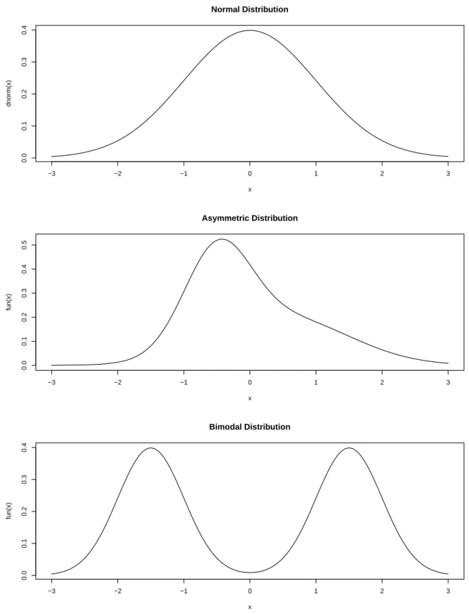
replications, each replication taking a random sample of size n = 500 with all random variables generated independently. We consider 6 data generating processes (DGPs) as follows:
Data Generating Process for Monte Carlo Experiment ("i; vi)–Distributions
Gaussian Asymmetric Bimodal
2
v(zi) = 1 Model 1 Model 3 Model 5
2
v(zi) = &(1 +kzik2)2 Model 2 Model 4 Model 6
Speci…cally, Models 1, 3 and 5 correspond to homoskedastic (in vi) DGPs, while Models 2, 4
and 5 correspond to heteroskedastic (in vi) DGPs. For the latter models, the constant & was
chosen so that E[v2
i] = 1. The three distributions considered for the unobserved error terms "i
and vi are: the standard Normal (labelled “Gaussian”) and two Mixture of Normals inducing
either an asymmetric or a bimodal distribution; their Lebesgue densities are depicted in Figure 1. We explored other speci…cations for the regression functions, heteroskedasticity form, and distributional assumptions, but we do not report these additional results because they were qualitative similar to those discussed here.
The estimators considered in the Monte Carlo experiment are constructed using power series approximations. We do not impose additive separability on the basis, though we do restrict the interaction terms to not exceed degree 5. To be speci…c, we consider the following
polynomial basis expansion:
Polynomial Basis Expansion: dz = 5 and n = 500
K pK(zi) K=n 6 (1; z1i; z2i; z3i; z4i; z5i)0 0:012 11 (p6(zi)0; z1i2; z2i2; z3i2; z4i2; z5i2)0 0:022 21 p11(zi) + …rst-order interactions 0:042 26 (p21(zi)0; z1i3; z2i3; z3i3; z34i; z5i3)0 0:052 56 p26(zi) + second-order interactions 0:112 61 (p56(zi)0; z1i4; z2i4; z3i4; z44i; z5i4)0 0:122 126 p61(zi) + third-order interactions 0:252 131 (p126(zi)0; z1i5; z2i5; z3i5; z4i5; z5i5)0 0:262 252 p131(zi) + fourth-order interactions 0:504 257 (p252(zi)0; z1i6; z2i6; z3i6; z4i6; z5i6)0 0:514 262 (p257(zi)0; z1i7; z2i7; z3i7; z4i7; z5i7)0 0:524 267 (p262(zi)0; z1i8; z2i8; z3i8; z4i8; z5i8)0 0:534 272 (p267(zi)0; z1i9; z2i9; z3i9; z4i9; z5i9)0 0:544 277 (p272(zi)0; z1i10; z2i10; z3i10; z4i10; z5i10)0 0:554
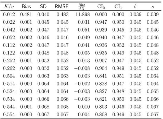
Thus, our simulations explore the consequences of introducing many terms in the partially linear model by varying K on the grid above from K = 6 to K = 277, which gives a range for K=n of f0:012; ; 0:554g. For each point on the grid of K=n, we report average bias, average standard deviation, mean square error and average standardized bias of ^ across simulations. We also consider the coverage error rates and interval length for two asymptotic 95% con…dence intervals: CI0 = " ^ 1 1 =2 ^ ^n1=2 p n ; ^ + 1 1 =2 ^ ^n1=2 p n # ; CI1 = " ^ 1 1 =2 s^n1=2 p n ; ^ + 1 1 =2 s^n1=2 p n # ;
where ^2 = (n d K)s2=n, and u1 = 1(u)denotes the inverse of the Gaussian
the homoskedasticity-consistent variance estimators without and with degrees of freedom correction, respectively.
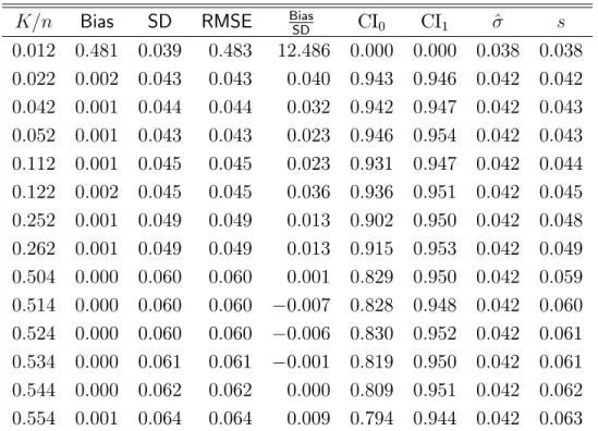
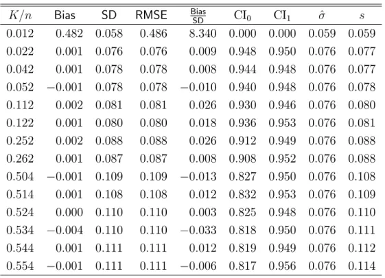
The main …ndings from the Monte Carlo experiment are presented in Tables 1–3. All results are consistent with the theoretical conclusions presented in the previous section. First, the results for standard Normal and non-Normal errors are qualitatively similar. This indicates that the Gaussian approximation obtained in Theorem1is a good approximation in …nite samples, even when K is a nontrivial fraction of the sample size. Second, as expected, a small choice of K leads to important smoothing biases. This a¤ects the …nite sample properties of the point estimators as well as the distributional approximations obtained in this paper. In particular, it a¤ects the empirical size of all the con…dence intervals. Third, in all cases the results under homoskedasticity or heteroskedasticity in vi are qualitatively
similar, showing that our theoretical results provide a good …nite sample approximation in both cases, even when K is a nontrivial fraction of the sample size. Fourth, as suggested by Theorem2, con…dence intervals without degrees of freedom correction (CI0) are under-sized,
while the con…dence intervals with degrees of freedom correction (CI1) have close-to-correct
empirical size in all cases. This result shows that the degrees of freedom correction is crucial to achieve close-to-correct empirical size when K=n is non-negligible.
In conclusion, we found in our small-scale simulation study that our theoretical results for the partially linear model with possibly many terms provide good approximation in samples of moderate size. In particular, under homoskedasticity of "i, we showed that con…dence
intervals constructed using s2 exhibit good empirical coverage even when K=n is “large”. We
also con…rmed that the Gaussian distributional approximation given in Theorem1represents well the …nite sample distribution of ^ even when K=n is “large”.
In Cattaneo, Jansson, and Newey (2015) we analyze in detail the case of (conditional) heteroskedasticity in "i, which requires the use of a new standard error formula, and also
compare those results to the case of homoskedasticity analyzed herein. We do not reproduce those results here to avoid repetition.
5
Conclusion
This paper showed asymptotic normality and gave consistent standard errors for coe¢ cients of interest when the number of covariates grows as fast as the sample size. It was also shown how this asymptotics has a similar structure to previously established results for many instrument asymptotics or small bandwidths. These results are all based on results for degenerate U-statistics, where asymptotic normality happens when the number of covariates
Our results apply to a class of semiparametric estimators ^ satisfying p
n(^ 0) = ^n1Sn+ op(1);
where ^n and Sn take a particular V-stastistic form, as discussed in Section 2. This class
of semiparametric estimators covers several interesting problems, but it is by no means exhaustive. For example, Cattaneo and Jansson (2015) show that a large class of (kernel-based) semiparametric estimators admit an expansion of the form
p
n(^ 0) = ^n1Sn Bn+ op(1);
where the bias term Bn is quantitatively and conceptually distinct from the smoothing bias
Bn described in Section 2 and, crucially, dominates the quadratic term Un arising from the
V-statistic Sn; that is, Un = op(Bn) in that setting. Nevertheless, the structure we have
considered in this paper is useful, providing new results for the partially linear model and a common structure for disparate literatures on many instruments and small bandwidths.
Finally, as a reviewer pointed out, the alternative asymptotics discussed in this paper are also qualitative distinct, but conceptually similar, to that encountered in the recent literature on “large”panel data models where the number of units n and the number of periods T are proportional; see, for example, Alvarez and Arellano (2003), Hahn and Newey (2004) and references therein. Speci…cally, whereas the “large-(n; T ) asymptotics” lead to the presence of a …rst-order bias in the distributional approximation (centering), the alternative asymp-totics discussed in this paper lead to a change in the …rst-order variance of the distributional approximation (scale). Therefore, the “large-(n; T ) asymptotics”in panel data contexts are more closely related to those obtained in Cattaneo and Jansson (2015) for non-linear semi-parametric problems, than to the distribution theory emerging from the common structure highlighted in this paper.
Appendix A: Proofs
All statements involving conditional expectations are understood to hold almost surely. Quali…ers such as “a.s.” will be omitted to conserve space. Throughout the appendix, C will denote a generic constant that may take di¤erent values in each case.
Assumption PLM and the Markov inequality, tr(1 nH 0M H) = min h2RK d 1 n n X i=1 kh(zi) 0hpK(zi)k2 = Op(K 2 h)!p 0: Also, V0V =n = O
p(1) by Assumption PLM and the Markov inequality, so by the
Cauchy-Schwarz inequality and M idempotent, kH0M V =nk [tr(H0M H=n) tr(V0V =n)]1=2
!p 0:By
the triangle inequality, we then have
^ n = 1 nX 0M X = 1 n(V + H) 0M (V + H) = 1 nV 0M V + o p(1):
Next, by Lemma A1 of Chao, Swanson, Hausman, Newey, and Woutersen(2012), 1 nV 0M V = 1 n n X i=1 Miivivi0+ 1 n n X i=1 n X j=1;j6=i Mijvivj0 = 1 n n X i=1 Miiviv0i+ op(1):
Finally, by the Markov inequality and using E[n 1Pni=1Miivivi0jZ] = n,
1 n n X i=1 Miivivi0 n!p 0
because Assumption PLM implies that vivi0 and vjvj0 are uncorrelated conditional on Z and
that E[M2
iikvik4jZ] C.
Proof of Lemma 2. Let G = [g1; : : : ; gn]0 and " = ["1; : : : ; "n]0. By the Cauchy-Schwarz
inequality, M idempotent, Assumption PLM, and the Markov inequality,
kn1G0M Hk r tr(1 nG0M G) r tr(1 nH0M H) = Op(K g h); which gives Bn= G0M H=pn = Op(pnK g h). Also, Rn = (V0M G + H0M ")=pn = Op(K g + K h) = op(1) because E[kp1 nV 0M Gk2 jZ] = 1 nG 0M E[V V0jZ]MG C1 nG 0M G = O p(K 2 g) and E[kp1 nH 0M "k2 jZ] = tr(1 nH 0M E[""0jZ]MH) C tr(1 nH 0M H) = O p(K 2 h)
Proof of Theorem 1. By Lemma A2 of Chao, Swanson, Hausman, Newey, and Woutersen (2012), 1=2 n 1 p n n X i=1 n X j=1 Mijvi"j !dN (0; Id)
under Assumption PLM. Combining this result with Lemmas1 and2, we obtain the results stated in the theorem.
Proof of Theorem 2. Let Y = [y1; : : : ; yn] and ^" = [^"1; : : : ; ^"n]0 = M (Y X ^). It
follows similarly to the proof of Lemma 1that 1 n" 0M " = 1 n n X i=1 Mii"2i + 1 n n X i=1 n X j=1;j6=i "iMij"j = 1 n n X i=1 MiiE["2ijzi] + op(1) = n K n 2 "+ op(1);
so it su¢ ces to show that ^"0^"=n = "0M "=n + o
p(1).
Lemma 1 and ^ = op(1) imply (^ )0X0M X(^ )=n = op(1), which together
with the Cauchy-Schwarz inequality and "0M "=n = O
p(1) gives 1 n(Y X ^ G) 0M (Y X ^ G) = 1 n" 0M " + 1 n(^ ) 0X0M X(^ ) 1 n2" 0M X(^ ) = 1 n" 0M " + o p(1): Similarly, G0M G=n = o
p(1) together with (Y X ^ G)0M (Y X ^ G)=n = Op(1) and
the Cauchy-Schwarz inequality gives 1 n^" 0^" = 1 n(Y X ^) 0M (Y X ^) = 1 n(Y X ^ G) 0M (Y X ^ G) + o p(1):
The conclusion follows by the triangle inequality.
Appendix B: Extension to Two-step Estimation
The common structure highlighted in Section2, and later used to study IV models with may instruments, kernel-based semiparametric estimators and the series-based semiparametric semi-linear model, can be extended to account for preliminary estimation. This extension, though conceptually not di¢ cult, may be important in series-based sample selection models as discussed in Newey (2009), or kernel-based estimators as discussed in Aradillas-Lopéz,
Honoré, and Powell (2007) and Escanciano and Jacho-Chavez (2012). In this appendix we discuss this extension heuristically, but relegate a formal analysis for future work.
Following the ideas and notation introduced in Section 2, consider a generic estimator ^(^) of the parameter 0 = 0( 0)2 Rd. In this appendix, the notation ^(^) (as opposed to
^) makes explicit that the estimator depends on an estimator ^ of the unknown “parameter”
0 2 , not necessarily …nite dimensional. As a natural generalization of (2) we then assume
that p n(^( ) 0) = ^n( ) 1Sn( ), Sn( ) = n X i=1 n X j=1 unij(Wi; Wj; ).
The exact form of unij(Wi; Wj; ) is context speci…c; unij(Wi; Wj) = unij(Wi; Wj; 0) in Section
2 and other examples are given in the references above. Suppose, in addition, that the estimator ^ is consistent in the sense that k^ 0k = op(1), where k k is some context
speci…c norm (e.g., if Rm
then k k will typically be the Euclidean norm).
It follows from the discussion in the paper, that the limiting distribution ofpn(^(^) 0) is determined by Sn(^) whenever ^n( 0) 1 n !p Id and ^n( 0) 1^n(^) !p Id. In many
cases, the latter assumption only imposes a consistency requirement (without a rate) on the estimator ^ and is therefore not particularly restrictive. The term Sn(^) can be handled, for
example, by employing the obvious decomposition
Sn(^) = Fn(^) + Sn; Fn( ) = Sn( ) Sn( 0); Sn= Sn( 0);
where now the asymptotic distributional approximation for Sn(^) is explained by the
…rst-step estimation contribution Fn(^), and the “oracle” term Sn already studied in the main
paper.
The additional term Fn(^) may be analyzed in multiple ways. For example, if ^ is
…nite-dimensional,pn-consistent, and some regularity conditions hold (including 7! unij(w1; w2; )
su¢ ciently “smooth” and well-behaved), then it may be shown that
Fn(^) F_n(^) = op(n 1=2), F_n(^) = n X i=1 n X j=1 _unij(Wi; Wj; 0) ! ^ 0 , where _un
ij(w1; w2; 0) is some function. For instance, _unij(w1; w2; 0) = @unij(w1; w2; 0)=@
if 7! un
ij(w1; w2; ) is di¤erentiable or, otherwise, _uijn(w1; w2; 0) may be obtained using
U-process theory.
where ^n= n X i=1 n X j=1 _unij(Wi; Wj; 0):
This illustrates how the discussion given in the main text may be extended to the case of two-step estimation. Assuming the …rst-step estimator ^ is pn-consistent (as will be the case whenever it is regular), it follows that the …rst step makes a non-negligible contribution to the asymptotic distribution unless the “orthogonality”condition ^n= op(n2)is satis…ed.
Formalizing the above ideas is beyond the scope of this paper, but we conjecture it can be done in fairly large generality, including some cases where ^ is in…nite dimensional and (possibly) notpn-consistent.
References
Alvarez, J., and M. Arellano (2003): “The Time Series and Cross-section Asymptotics of Dynamic Panel Data Estimators,” Econometrica, 71(4), 1121–1159.
Angrist, J., G. W. Imbens, andA. Krueger (1999): “Jackknife Instrumental Variables Estimation,” Journal of Applied Econometrics, 14(1), 57–67.
Aradillas-Lopéz, A., B. E. Honoré, and J. L. Powell (2007): “Pairwise Di¤erence Estimation with Nonparametric Control Variables,” International Economic Review, 48, 1119–1158.
Atchadé, Y. F., and M. D. Cattaneo (2014): “A Martingale Decomposition for Quadratic Forms of Markov Chains (with Applications),” Stochastic Processes and their Applications, 124(1), 646–677.
Bekker, P. A. (1994): “Alternative Approximations to the Distributions of Instrumental Variables Estimators,” Econometrica, 62, 657–681.
Belloni, A., V. Chernozhukov, D. Chetverikov, and K. Kato (2015): “On the Asymptotic Theory for Least Squares Series: Pointwise and Uniform Results,”Journal of Econometrics, 186(2), 345–366.
Belloni, A., V. Chernozhukov, and C. Hansen (2014): “Inference on Treatment E¤ects after Selection among High-Dimensional Controls,” Review of Economic Studies, 81(2), 608–650.
Cattaneo, M. D., R. K. Crump, and M. Jansson (2010): “Robust Data-Driven In-ference for Density-Weighted Average Derivatives,” Journal of the American Statistical Association, 105(491), 1070–1083.
(2014a): “Bootstrapping Density-Weighted Average Derivatives,” Econometric Theory, 30(6), 1135–1164.
(2014b): “Small Bandwidth Asymptotics for Density-Weighted Average Deriva-tives,” Econometric Theory, 30(1), 176–200.
Cattaneo, M. D., and M. H. Farrell (2013): “Optimal Convergence Rates, Bahadur Representation, and Asymptotic Normality of Partitioning Estimators,”Journal of Econo-metrics, 174(2), 127–143.
Cattaneo, M. D.,andM. Jansson (2015): “Bootstrapping Kernel-Based Semiparametric Estimators,” working paper, University of Michigan.
Cattaneo, M. D., M. Jansson, and W. K. Newey (2015): “Treatment E¤ects With Many Covariates and Heteroskedasticity,” working paper, University of Michigan.
Chao, J. C., N. R. Swanson, J. A. Hausman, W. K. Newey, and T. Woutersen (2012): “Asymptotic Distribution of JIVE in a Heteroskedastic IV Regression with Many Instruments,” Econometric Theory, 28(1), 42–86.
Chen, X. (2007): “Large Sample Sieve Estimation of Semi-Nonparametric Models,” in Handbook of Econometrics, Volume VI, ed. by J. Heckman, and E. Leamer, pp. 5550– 5632. Elsevier Science B.V.
de Jong, P. (1987): “A Central Limit Theorem for Generalized Quadratic Forms,”Proba-bility Theory and Related Fields, 75, 261–277.
Donald, S. G., and W. K. Newey (1994): “Series Estimation of Semilinear Models,” Journal of Multivariate Analysis, 50(1), 30–40.
El Karoui, N., D. Bean, P. J. Bickel, C. Lim, and B. Yu (2013): “On Robust Regression with High-Dimensional Predictors,” Proceedings of the National Academy of Sciences, 110(36), 14557–14562.
Escanciano, J. C., and D. Jacho-Chavez (2012): “pn-Uniformly Consistent Density Estimation in Nonparametric Regression,” Journal of Econometrics, 167(1), 305–316.
Giné, E., and R. Nickl (2008): “A Simple Adaptive Estimator of the Integrated Square of a Density,” Bernoulli, 14(1), 47–61.
Hahn, J., and W. K. Newey (2004): “Jackknife and Analytical Bias Reduction for Non-linear Panel Data Models,” Econometrica, 72(4), 1295–1319.
Hansen, C., J. Hausman, and W. K. Newey (2008): “Estimation with Many Instru-mental Variables,” Journal of Business and Economic Statistics, 26(4), 398–422.
Heckman, J. J., and E. J. Vytlacil (2007): “Econometric Evaluation of Social Pro-grams, Part I: Causal Models, Structural Models and Econometric Policy Evaluation,”in Handbook of Econometrics, vol. VI, ed. by J. Heckman, and E. Leamer, pp. 4780–4874. Elsevier Science B.V.
Huber, P. J. (1973): “Robust Regression: Asymptotics, Conjectures, and Monte Carlo,” Annals of Stastistics, 1(5), 799–821.
Imbens, G. W., and J. M. Wooldridge (2009): “Recent Developments in the Econo-metrics of Program Evaluation,” Journal of Economic Literature, 47(1), 5–86.
Kunitomo, N. (1980): “Asymptotic Expansions of the Distributions of Estimators in a Linear Functional Relationship and Simultaneous Equations,” Journal of the American Statistical Association, 75(371), 693–700.
Li, Q., and S. Racine (2007): Nonparametric Econometrics. Princeton University Press, New Yersey.
Linton, O. (1995): “Second Order Approximation in the Partialy Linear Regression Model,” Econometrica, 63(5), 1079–1112.
Morimune, K. (1983): “Approximate Distributions of k-Class Estimators when the Degree of Overidenti…ability is Large Compared with the Sample Size,” Econometrica, 51(3), 821–841.
Newey, W. K. (1997): “Convergence Rates and Asymptotic Normality for Series Estima-tors,” Journal of Econometrics, 79, 147–168.
(2009): “Two-Step Series Estimation of Sample Selection Models,” Econometrics Journal, 12(1), S217–S229.
Newey, W. K., F. Hsieh, and J. M. Robins (2004): “Twicing Kernels and a Small Bias Property of Semiparametric Estimators,” Econometrica, 72(1), 947–962.
Powell, J. L., J. H. Stock, and T. M. Stoker (1989): “Semiparametric Estimation of Index Coe¢ cients,” Econometrica, 57(6), 1403–1430.
Schick, A., and W. Wefelmeyer (2013): “Uniform Convergence of Convolution Esti-mators for the Response Density in Nonparametric Regression,”Bernoulli, 19(5B), 2250– 2276.
van der Vaart, A. W. (1998): Asymptotic Statistics. Cambridge University Press, New York.
−3 −2 −1 0 1 2 3 0.0 0.1 0.2 0.3 0.4 Normal Distribution x dnor m(x) −3 −2 −1 0 1 2 3 0.0 0.1 0.2 0.3 0.4 0.5 Asymmetric Distribution x fun(x) −3 −2 −1 0 1 2 3 0.0 0.1 0.2 0.3 0.4 Bimodal Distribution x fun(x)
Table 1: Simulation Results, Models 1 2, Gaussian Distribution. (a) Model 1: Homoskedastic vi
K=n Bias SD RMSE Bias
SD CI0 CI1 ^ s 0:012 0:481 0:040 0:483 11:898 0:000 0:000 0:039 0:039 0:022 0:001 0:045 0:045 0:031 0:947 0:950 0:045 0:045 0:042 0:002 0:047 0:047 0:051 0:939 0:945 0:045 0:046 0:052 0:002 0:046 0:046 0:049 0:940 0:947 0:045 0:046 0:112 0:002 0:047 0:047 0:041 0:936 0:952 0:045 0:048 0:122 0:000 0:048 0:048 0:005 0:935 0:949 0:045 0:048 0:252 0:001 0:052 0:052 0:013 0:907 0:947 0:045 0:052 0:262 0:000 0:052 0:052 0:008 0:904 0:949 0:045 0:052 0:504 0:000 0:063 0:063 0:003 0:841 0:951 0:045 0:064 0:514 0:000 0:064 0:064 0:002 0:828 0:947 0:045 0:064 0:524 0:000 0:064 0:064 0:003 0:827 0:948 0:045 0:065 0:534 0:000 0:066 0:066 0:003 0:821 0:950 0:045 0:066 0:544 0:001 0:068 0:068 0:010 0:803 0:946 0:045 0:067 0:554 0:000 0:067 0:067 0:004 0:808 0:949 0:045 0:067 (b) Model 2: Heteroskedastic vi
K=n Bias SD RMSE BiasSD CI0 CI1 ^ s
0:012 0:483 0:046 0:485 10:460 0:000 0:000 0:039 0:040 0:022 0:002 0:045 0:045 0:034 0:949 0:953 0:045 0:046 0:042 0:001 0:046 0:046 0:015 0:946 0:949 0:045 0:046 0:052 0:002 0:046 0:046 0:034 0:947 0:955 0:045 0:046 0:112 0:001 0:049 0:049 0:015 0:932 0:950 0:045 0:048 0:122 0:001 0:049 0:049 0:025 0:929 0:946 0:045 0:049 0:252 0:000 0:052 0:052 0:009 0:914 0:951 0:046 0:053 0:262 0:001 0:053 0:053 0:025 0:915 0:952 0:046 0:054 0:504 0:000 0:068 0:068 0:002 0:827 0:947 0:048 0:068 0:514 0:001 0:068 0:068 0:019 0:829 0:953 0:048 0:068 0:524 0:003 0:068 0:069 0:050 0:824 0:953 0:047 0:069 0:534 0:000 0:070 0:070 0:003 0:819 0:949 0:048 0:070 0:544 0:002 0:070 0:070 0:024 0:819 0:948 0:048 0:071 0:554 0:000 0:074 0:074 0:004 0:801 0:943 0:048 0:072 Notes:
(i) columns Bias, SD, RMSE and Bias
SD report, respectively, average bias, average standard deviation, root
Table 2: Simulation Results, Models 3 4, Asymmetric Distribution. (a) Model 3: Homoskedastic vi
K=n Bias SD RMSE Bias
SD CI0 CI1 ^ s 0:012 0:481 0:039 0:483 12:486 0:000 0:000 0:038 0:038 0:022 0:002 0:043 0:043 0:040 0:943 0:946 0:042 0:042 0:042 0:001 0:044 0:044 0:032 0:942 0:947 0:042 0:043 0:052 0:001 0:043 0:043 0:023 0:946 0:954 0:042 0:043 0:112 0:001 0:045 0:045 0:023 0:931 0:947 0:042 0:044 0:122 0:002 0:045 0:045 0:036 0:936 0:951 0:042 0:045 0:252 0:001 0:049 0:049 0:013 0:902 0:950 0:042 0:048 0:262 0:001 0:049 0:049 0:013 0:915 0:953 0:042 0:049 0:504 0:000 0:060 0:060 0:001 0:829 0:950 0:042 0:059 0:514 0:000 0:060 0:060 0:007 0:828 0:948 0:042 0:060 0:524 0:000 0:060 0:060 0:006 0:830 0:952 0:042 0:061 0:534 0:000 0:061 0:061 0:001 0:819 0:950 0:042 0:061 0:544 0:000 0:062 0:062 0:000 0:809 0:951 0:042 0:062 0:554 0:001 0:064 0:064 0:009 0:794 0:944 0:042 0:063 (b) Model 4: Heteroskedastic vi
K=n Bias SD RMSE BiasSD CI0 CI1 ^ s
0:012 0:485 0:046 0:488 10:566 0:000 0:000 0:038 0:038 0:022 0:001 0:042 0:042 0:031 0:947 0:949 0:042 0:043 0:042 0:001 0:043 0:043 0:025 0:946 0:951 0:042 0:043 0:052 0:002 0:044 0:044 0:047 0:937 0:943 0:042 0:043 0:112 0:002 0:045 0:045 0:037 0:933 0:945 0:043 0:045 0:122 0:001 0:046 0:046 0:025 0:929 0:945 0:043 0:046 0:252 0:000 0:050 0:050 0:004 0:910 0:949 0:043 0:050 0:262 0:001 0:050 0:050 0:020 0:907 0:951 0:043 0:050 0:504 0:000 0:064 0:064 0:002 0:832 0:947 0:045 0:064 0:514 0:001 0:065 0:065 0:008 0:827 0:948 0:045 0:064 0:524 0:001 0:065 0:065 0:015 0:817 0:948 0:045 0:065 0:534 0:001 0:066 0:066 0:013 0:824 0:948 0:045 0:065 0:544 0:000 0:067 0:067 0:002 0:799 0:951 0:045 0:066 0:554 0:000 0:067 0:067 0:001 0:811 0:948 0:045 0:067 Notes:
(i) columns Bias, SD, RMSE and Bias
SD report, respectively, average bias, average standard deviation, root
mean square error, and average standarized bias of the estimator ^ across simulations;
(ii) columns CI0 and CI1 report empirical coverage for homoskedastic-consistent con…dence intervals,
Table 3: Simulation Results, Models 5 6, Bimodal Distribution. (a) Model 5: Homoskedastic vi
K=n Bias SD RMSE Bias
SD CI0 CI1 ^ s 0:012 0:482 0:058 0:486 8:340 0:000 0:000 0:059 0:059 0:022 0:001 0:076 0:076 0:009 0:948 0:950 0:076 0:077 0:042 0:001 0:078 0:078 0:008 0:944 0:948 0:076 0:077 0:052 0:001 0:078 0:078 0:010 0:940 0:948 0:076 0:078 0:112 0:002 0:081 0:081 0:026 0:930 0:946 0:076 0:080 0:122 0:001 0:080 0:080 0:018 0:936 0:953 0:076 0:081 0:252 0:002 0:088 0:088 0:026 0:912 0:949 0:076 0:088 0:262 0:001 0:087 0:087 0:008 0:908 0:952 0:076 0:088 0:504 0:001 0:109 0:109 0:013 0:827 0:950 0:076 0:108 0:514 0:001 0:108 0:108 0:012 0:832 0:953 0:076 0:109 0:524 0:000 0:110 0:110 0:003 0:825 0:948 0:076 0:110 0:534 0:004 0:110 0:110 0:033 0:818 0:950 0:076 0:111 0:544 0:001 0:111 0:111 0:012 0:819 0:949 0:076 0:112 0:554 0:001 0:111 0:111 0:006 0:817 0:956 0:076 0:114 (b) Model 6: Heteroskedastic vi
K=n Bias SD RMSE BiasSD CI0 CI1 ^ s
0:012 0:483 0:062 0:487 7:811 0:000 0:000 0:059 0:060 0:022 0:001 0:077 0:077 0:011 0:945 0:948 0:076 0:077 0:042 0:001 0:077 0:077 0:011 0:945 0:951 0:076 0:078 0:052 0:001 0:079 0:079 0:009 0:941 0:948 0:077 0:079 0:112 0:000 0:082 0:082 0:001 0:938 0:954 0:077 0:082 0:122 0:004 0:080 0:080 0:046 0:942 0:955 0:077 0:082 0:252 0:000 0:092 0:092 0:002 0:904 0:946 0:078 0:090 0:262 0:002 0:089 0:089 0:026 0:910 0:957 0:078 0:091 0:504 0:001 0:117 0:117 0:005 0:826 0:946 0:080 0:114 0:514 0:002 0:116 0:116 0:017 0:828 0:951 0:081 0:116 0:524 0:000 0:118 0:118 0:003 0:821 0:945 0:081 0:117 0:534 0:001 0:118 0:118 0:010 0:815 0:953 0:081 0:119 0:544 0:000 0:119 0:119 0:003 0:816 0:952 0:081 0:120 0:554 0:000 0:125 0:125 0:001 0:797 0:943 0:081 0:121 Notes:
(i) columns Bias, SD, RMSE and Bias
SD report, respectively, average bias, average standard deviation, root