Conditional extremes and near-extremes

Digitized

by

the

Internet

Archive

in

2011

with

funding

from

Boston

Library

Consortium

Member

Libraries

I

Dewey

B31

^415

-21

Massachusetts

Institute

of

Technology

Department

of

Economics

Working

Paper

Series

CONDITIONAL

EXTREMES

AND

NEAR-EXTREMES

Victor

Chemozhukov,

MIT

Working

Paper

01

-21

July

2000

RoomE52-251

50

Memorial

Drive

Cambridge,

MA

02142

This

paper

can

be

downloaded

without

charge

from

the

Social

Science

Research Network

Paper

Collection

at

MASSACHUSEHS

INSTITUTE OF

TECHNOLOGY

AUG

1 5 2001

Massachusetts

Institute

of

Technology

Department

of

Economics

Working

Paper

Series

CONDITIONAL

EXTREMES

AND

NEAR-EXTREMES

Victor

Chemozhukov,

MIT

Working

Paper

01-21

July

2000

Room

E52-251

50

Memorial

Drive

Cambridge,

MA

02142

This

paper

can

be

downloaded

without

charge

from

the

Social

Science

Research

Network

Paper

Collection

at

CONDITIONAL

EXTREMES

AND

NEAR-EXTREMES

Victor

Chernozhukov^

Dept. of

Economics,

MIT,

E52-262F,

Cambridge,

MA,

02142

email:

vchern@mit.edu

Version:

May

10, 2001 First Version: October, 1998

Abstract

This

paper

develops a theory of high

and

low (extremal) quantile regression: the linear models, estimation,

and

inference. In particular, the

models

coherently

com-bine theconvenient, flexible linearity with the extreme-value-theoretic restrictions

on

tails

and

the general heteroscedasticity forms.

Within

these models, thelimit lawsfor

extremal quantile regression statistics are obtained

under

the rank conditions (exper-iments) constructed to reflect the extremal or rarenature oftail events.

An

inference

framework

is discussed.

The

results apply to cross-section (and possibly dependent) data.

The

applications, ranging

from

the analysis of babies' very low birthweights, (5,s) models, tail analysis in heteroscedastic regression models, outlier-robust infer-ence in auction models,

and

decision-making

under extreme

uncertainty, provide the motivation

and

applications ofthistheory.

Key

Words: Quantile

Regression

'©July 2000 V. Chernozhukov. Rights Reserved. This paperisa partof

my

Ph.D. dissertation at Stanford, completed in 2000. I

am

very grateful to Takeshi Amemiya, Roger Koenker,

Thomas

MaCurdy, Mordecai Kurz, and also to Anil Bera, Stephen Portnoy,

Thomas

Sargent for advise and

help;Pat Bajari, JosephRomano,Keith Knight, and JanaJureckova, fordiscussionsand from

whom

I learned a great deal; and also friends: IgorMakarov, Stijn Van Nieuwerburgh, Leonardo Rezende, Michael Schwarz, and Lei Zhang, and especially Han Hong, Robert McMillan, Sergei Morozov, and Len Umancev. I thank also the seminar participants at Brown, Caltech, Chicago,

CIRANO,

Duke, Mannheim, MIT-Harvard, Northwestern, Stanford,

UCLA, UCSD,

University ofIllinois, Yale, and Neuchatel

May

2000 Conference on Recent Developments in Regression,

CEME

2001 Conference, Conference on Economic Applications ofQuantile Regression in Konstanz, 2000, especially J.

An-grist, D.Andrews, J. Altonji, M. Buchinsky, P. Christophersen, F. Diebold, G. Elliot, R. Engle,

B.Fitzenberger, C. Granger, J. Hahn, J. Hamilton, L. Hansen, M. Hallin, J.Heckman, G. Imbens, D. Jorgenson, T.Bollerslev, C. Manski, R. Matzkin, P. Phillips,J. Rust, R. Sherman, D. Strook, G. Tauchen, R. Tsay,J. Jureckova, and H.White. 1 alsothank JerryHausman, GuidoKursteiner,Ziad

Nejmeldeen, and Whitney Newey for suggestions that drastically improved the presentation of the

material; and also

Bo

Honore and Charles Manski for suggesting to look into modeling questions

carefully.

I gratefullyacknowledge thefinancialsupport provided by the Alfred P. Sloan Dissertation

Contents

1

Introduction

1

2

Econometric

Applications

3

3

Extremal

Quantiles

and

Rank

Sequences

6

3.1 Extremal Conditional Quantiles 6 3.2 Linear Quantile Regression

Model

7 3.3

Sample

Regression Quantile Statistics 7 3.4 Extremes, Near-Extremes

&

Data

Scarcity 8 3.5 TailTypes, Support Types,and Classical Limits 9

3.6 Limit DistributionsofOrdinary

Sample

Quantiles 9

4

The

Extremal

Regression Quantile

Models

11

4.1

Model

1; Tail Homogeneity 11

4.2

Model

2: Congenial TailHeterogeneity 13

5

Asymptotics

under

Extreme Ranks

15

6

Asymptotics under

Intermediate

Ranks

20

7 Inference 23

A

Useful

background

27

A.l Point processes 27

A.2

Convex

Semi-ContinuousObjectives 27

B

Proofs

for section 5,

extreme

ranks

28

B.l Detailsand definitions 28 B.2 Basic conditionsfor nondegenerate asymptotics 29 B.3 Limits in Models 1 and2 32

C

Proofs

for section 6,

intermediate

ranks

33

C.l Basic conditionsfor a normallimit 33 C.2 Limits in Models1 and2 34

D

Properties

of

Models

1

and

2

36

1

Introduction

Regression quantiles,

Koenker and

Bassett[48], represent a flexible

and

informative

method

of regression analysis as they describe the conditional distribution ofthe

re-sponsevariable

Y

givencovariate

X

,without

imposing

rigiddistributionalassumptions.

The

goal ofthis

paper

is to

model

and

make

inference

on

the extremal {near-extreme high or low) regression quantile functions. In essence, they represent the

models

of the extremal values of

Y

conditional

upon X.

For example, the near-extreme 0.1-th conditional quantile function describes the values

below

which

Y

fallswith probability

10%

given values of

X.

Modeling

high orlow conditional quantiles is motivated

by

many

examples.

Some

include: (i) in micro- economics: (5,s)

models

ofinvestment, inventory,

employment

shortages; auction models, reservation

wage

equations; (ii) in finance, micro-

and

macro-

economics: decision-making

under

extreme

uncertainty,

where

good

risk

mea-sures are vital for the purposesofinsurance, safety-first resource allocation,

and

man-agement

ofrisks;

and

many

others.

The

ordinaryextremalquantiles, the

models

and

the

sample

analogs,

have been

the

main

subject ofclassical

and

modern

extreme

value theory,

which

forms

an important

field ofapplied

and

theoretical statistics.'^

The

theory

was

developed

by

Von

Mises,

Prechet, Fisher,

Gnedenko,

Smirnov, de

Haan, and

many

others.

The

ordinary

sample

quantiles

have

an

immense

inference role, providing the estimators of the tail index

and

othertailfunctionals (Pickands[57],Hill[40],

Dekkers

and

de Haan[21]).

Analogous

motivations underliethe present analysis aswell.

Inthis

paper

we

study theextremal (high

and

low)conditional quantiles- thelinear models

and

the

sample

regression analogs. In particular,the

models

coherently

combine

convenient, flexible linearity with the extreme-value-theoretic restrictions

on

tails

and

thegeneral heteroscedasticity forms.

Within

these models, the limitlawsfor extremal quantile regression statistics are obtained

under

the rank conditions constructed to reflectthe extremal or rare nature oftail events.

The

goal is the practical,

important

problem

ofmodeling

and

making

inference

on

the .3-th

and

lower

and

.7-th

and

higher regression quantiles, as well asconducting the tail inference, inthe

common

economic

data

sets.^

{Our

target is not the "exotic" 0-th quantile.)

The

rank conditions

approximate

thedegreesof lack ofdataor extremality pertinent tothe inference

about

the quantiles ofinterest. Define rank r asthe quantile index r times the

sample

size T.

The

extreme

and

intermediate

rank

conditions apply to the cases

where

index t is extremal(e.g. .1, .2)

and

is low(rissmall) or notlow {rislarge) relativetothe

sample

sizeT.^ Formally,the sequenceofthe quantileindex-samplesize pairs {tt,T) is

an

extreme rank sequence if

(i) Tr

\

0,

TrT

-^

k>

0,

and an

intermediate rank sequenceif

{ii) T-r

\

0,

TtT

—

> GO.

-Asoftoday, thousandsofpapers aredevotedto theextremevaluetheory.

Many

excellent books

givesystematic treatments. Seee.g. [7], [64], [65], [52], [33], [34], [26], [73].

^Say with

T

<

3000, and typical number of regressors,

5—10

and higher.

Because

the principles (i)

and

(ii) constructively exploit that the relevant data is

formed

by the tail events and, oris scarce, they lead to

a. asymptotic distributions that either fit the finite-sample distributions better or are

more

parsimonious than the conventional approximations,

b.

important

tailinferences, based

on

the extremal regression quantiles.

In evaluatingthese concepts, it is

important

to keep in

mind

that these alternative sequences are designedto yield better approximations ingiven practical

problems

with given

sample

sizes,even

when

the quantile indexis not very low.

And,

incase(a), it is

completely irrelevant

whether

or notfuture

sampling

will lead to

samples

conforming

tothese sequences or not.

The

concepts (i)

and

(ii) are well

motivated

by

theintellectual

and

practical success ofthe

extreme

value theory,

which

focused

on

theordinary

sample

quantiles.

The

con-cepts are also similar in spirittoother "alternative" asymptotics, e.g.,

GMM

when

the

number

of

moment

conditionsislarge;

weak

instrumentstheory,

where

theinstruments

are

weakly

correlatedwith the regressors; near-to-unit root theory; and, generally, the theory ofstatistical experiments.

The

organization

and

contribution ofthis

paper

is eis follows:

1. Section 2

demonstrates

the relevanceofthe

problem

in

economic

analysis.

2. Section 3 introduces the principles ofextremality for the regression quantiles

-namely

that ofthe intermediate

and extreme rank

sequences.

3. Section 4 develops the

models

oftheextremal (low) conditional quantiles.

They

coherently

combine

the linear functional forms with the extreme-value-theoretic

re-strictions,

and

lead to non-degenerate,

parsimonious

limit distributions.

The

models

are distribution-free

and

flexible, allowingfor sophisticatedeffects ofcovariates

on

the

shape

oftheconditional distribution (the scale, kurtosis, skewness, etc.). Importantly, these

models

do not admitreductions to theclassical

one-sample

case (by

removing

the conditional

mean

and/or

scale).

4.

Within

the formulated models, section 5 provides the

asymptotic

limit theory for the

sample

regression quantiles

under

the

extreme rank

condition,

tT

—

) fc

>

0.^

The

Hmit

is driven

by

a stochastic integral ofa "residual" function with respect to a Poisson pointprocess.

5. Section6, using additionaltailrestrictions, providesthe

asymptotic

distributions of regression quantiles

under

the intermediate

rank

condition,

tT

—

>

oo,r

-^ 0.

The

limit is normal, with variance parsimoniously

determined

by

the tail indices. This enables a very practical inference. (In contrast, the conventional theory requires the

nonparametric

estimatesofthe conditionaldensity functionsevaluated at the extremal quantiles). This provides aregression

analogue

offairly recent results of

Dekkers and

de Haan[21].

^This paper is not about t

=

0, the linear programming estimator (also called 'extreme

regres-sion quantile'), considered in Feigin and Resnick[29], Portnoy and Jureckova[60], Chernozhukov[12],

Knight[47] within thelocation-shiftmodel(Covariatesonlyaffectthe locationbut not thescale,shape ortailofthe conditionaldistribution.) Theestimator, definedas

max

A''/3s.t. Yt

<

Xtf),Vtand useful as aboundaryestimate, can't be used at all in the present context.

We

look atdifferent estimators (high and lowregression quantiles) that have verydifferent asymptoticsand applications[t

>

(Tis

finite); seeexamples 2.1-2.4,where thesupport is unbounded or "boundaries" depend on unobserved

6.

We

conclude

by

discussing

an

inference theory

and an

empirical

paper

[15].

Also relevant are the

works

of Smith[73], Tsay[75],

and

references therein,

who

develop the

models

of exceedances over high constant thresholds.

The

parametric likelihoodof thePareto family is usedtodescribesuch data,

and parameters

are

made

dependent on

regressors. It should

be

clear that the goals, models,

and

methods

of this paper are quite different.

Our

analysis should be

viewed

as

complementing

the studyofthe central rank regression quantiles, with the motivation

stemming

from

the

wide

use ofquantile regression in data analysis in econometrics

and

statistics.

2

Econometric

Applications

Quantileregression is a popular tool ineconometric applications. See

Abadie

et al.[l],

Buchinsky[9], Chamberlain[ll],

Poterba

and

Rubin[61],

and

thereviewof

Koenker and

Hallock[50].

Our

results can beuseful in

about

any

such application,sinceourfocusis

the inference

about

high

and

low conditional quantiles (say .7

and

higher

and

.3

and

lower, in a typical data-set), recognizing the extremality

and/or

scarcity ofthe tail

events.

Important

inferences

about

the tail shapes can

be

made

as well.

There

are

many

examples,

where

high or low quantiles are of particular interest. For example, Abreveya[2]

and Koenker and

Hallock[50] characterize the

economic

determinants of babies' verylow birth-weights

through

thenear-extremeconditional quantiles (.05

and

below). Deaton[20]

examines

food expenditure ofPakistanihouseholds

by

the.1-th

and

.9 -th conditional quantiles.

The

following presents abriefdiscussion of

some

others.

Example

2.1

(Determinants

of

Generalized

{S,s)

Models.)

The

(5,s) theory is widely used in the firm-level

microeconomic

studies, including the analysis of durable

good

inventories,

employment

shortages,

and

investment in capitalgoods.

Lumpiness

ofadjustments, a

main

prediction, is well

documented.

E.g.,

Arrow

et al. [5], Scarf[71],

Rust

and

Hall[37], Aguirregabiria[3], Caballero [10].

Inthe (5,s) theory,afirm allowsastate variable Vj (capital stock,inventory) tofall

until itreaches a lower barrier, s{Xt), at

which

point the stock is replenished (jumps) to

an

upper

barrier, S{Xt).

Such

decisions are optimal in general settings (Hall

and

Rust[38]).

Xt

may

include prices

and

other variables that affect the firm's beliefs

about

future sales

and

costs (e.g. industrial production

and

commodity

price indices, interest rates).

Assume

that {Yt,Xt) areobserved for a cross-section offirms.

Absent

unobserved

heterogeneity, s{Xt)

and S{Xt)

are exactly the

minimal and

maximal

con-ditionalquantiles ofYt, given A''^. Otherwise, s{Xt)

and S{Xt)

arestill strongly related to the extremalconditional quantiles.

To

address the unobserved heterogeneity, Caballero

and

Engel[10] introduce the stochastic barriers [s{Xt)

—

Vt,S{Xt)

+

et] with

unobserved

time-

and

firm- specific

random

components

et,Vi.

They

propose probabilistic

adjustment

models

(hazard

functions) to describethe evolutionofYt across firms

and

or times. Insuch models, the high

and

low conditional quantiles also describe the probabilistic rules. For example, the inventory variable Yt is

below

the .1-th conditional quantileonly with probability

10%,

given A'(. Inference

about

such functions is exactly our area of focus.

More

generally,

we

can

map

quantile functions into

hazard

functions,

and

vice-versa.

de-Figure 1: (S,s) model with stochastic bands [s(.Y)

—

v,S{x)

+

e], where &

and

v are the unobserved firmand timespecific

random

components. Panel (A):

Data

on asinglefirm

may

be generated by discrete sampling from the time path of (Yi,Xt). E.g. Rust

and

Hall[37].

Panel (B);

Data

{Yi,Xi)

may

be generatedasa cross-section of plants. E.g. [3],[10],

terminants ofthe {S{x),s{x)) functions. Specifically,

suppose

that

[s{Xt)-vt,S(Xt)

+

et]

constitute the

adjustment

barriers, with Vt,et

>

0,s(A'j)

<

S{Xt)

a.s., so that the interval is non-empty.

The

timingis continuous. IfYj hits the lower

bound

s{Xt) —Vt,

it is adjusted to the

upper

bound

S{Xt)

+

et- Pairs {Yt,Xt) are the observed

draws

of different firms (or apanel, stationarity assumed). For brevity, let's focus

on

s{X).

Suppose

Vt

and

et are

independent

ofXt,^ then for c

>

0:

P{Yt

<

s{Xt)

-

c\Xt)

=

EPiXt

-

s{Xt)

< -c\Xt,c<

Vt)

P(c

<

vt)

+

EP{Yt

-

s{Xt)

< -c\Xt,c>

Vt)

P{c

>

Vt).

By

construction

P{Yt

—

s{Xt)

<

—c\Xt,c

>

vt)

=

0. Additionally,

impose

thefollowing

tail

homogeneity

condition: for all c

>

sufficiently closeto Uj:^

PiYt

-

s{Xt)

<

-c\Xt,c<

Vt)

=

a{vt

-

c). (2.1)

Thinking

ofYt

—

[s{Xt)

—

vt] as a positive "duration" variable, (2.1) states

an

"ac-celerated failure time"

model

for the tail (which is

more

general

than

in [10]). (2.1)

imposes

no

restrictions

on

the central features of the conditional distribution of Yt,

which

is reasonable, since the (5, s) theory does not relate the central features to the adjustment barriers. For

example,

the

symmetry

or homoscedasticity

assumptions

are unreasonable. This implies that for

—

c low

enough

and

some

low

constant (p{c)

P{Yt

-

siXt)

<

-c\Xt)

=

(Pic),

or, equivalently, that for small r

>

QY,{r\Xt

=

x)

=

s{x)

-

c{t)

This isreasonable, since S{X),s(x) incorporate thebarriercomponentthat depends on X.

Nev-ertheless, wecan allow e,vto bedependent on A'.

A

noteisavailableupon request.

istheT-th conditional quantile ofYt given Xt- Therefore,s{x) equalsthelow (extremal) conditional quantiles

up

to

an

additive constant. Notably, it isnotpossible toestimate s(x) offthe central features ofthe conditional distribution ofYt-, as discussed above.

The

inference

about

Qy{t\X)

for low values of r is exactly our area of focus.

The

analytical

examples

of

Rust and

Hall suggest that linear/polynomial functions are excellent descriptions of(s(x),5(x)) functions.

Example

2.2 (Tail

Analysis

in

Regression

Models)

The

tail

shape

(index) ofthe conditional distributionis

important

inthe regression analysis. Forexample, the thick-tailed distributions favor the

LAD

and

other estimators

more

than

the

OLS.

Thus,

knowing

the tail index helps determine betterestimators.

On

the otherhand, the tail

shapes are

important

in describing the large insurance claims ([26]), the analysis of

the long

and

short

term

survival

and

durations ([49], [42]),

and

financial data (e.g.

Mandelbrot[54], Fama[28],

Kearns

and

Pagan[45], Danielsson

and

de Vries[17]). In the non-regression setting, the tail index estimators of Hill

and

Pickands

have

been

countlessly used in the empiricalanalysis.

However,

estimation ofthetail index in the presence of the shape heteroscedasticity (scale, skewness, kurtosis,

and

other forms) is

largely

an

open, difficult problem.

Our

results allow

one

to construct the regression analogs ofthe Pickands

and

Hill tail indexestimators, based

on

theextremalregression quantiles,

which

specifically adapt tothe shape-heteroscedastic setting,

and

are simple in practice. Section 7 off'ers adiscussion,

and

[15] provides

an

empirical application.

Example

2.3

(Decision

Making

under

Extreme

Uncertainty)

Risk is a key

subject ofnon-financial

and

financial decisions, insurance,

and

regulation.

Both

the firms

and

the regulators are seriously concerned

about extreme

risks- the tail events that can

wipe

out capital, hinderingliquidity or solvency.

An

important

branch

of

economics

literatureis devotedtosafety-first decision

mak-ing. See Roy[68], Telser[74], Pyle

and

Turnovsky[63], Bertail et al[8]

and

others. In this approach, the decision-makers (firms, investors, regulators) solveeither:

1.

max

z, or 2.

max

/^(q),

where

If (a) is the

random

payoff (e.g. private or public benefits

and

profits) to the decision

a

(technology, portfolio composition, buffer stocks, quality/quantity offood control); z is the safety

margin

or disaster level of the payoff; r is the probability of the disaster or of exceeding the margin, set to

be

small; fi is the

mean

of ^''((q);

(5y,(a)(T|Xi) is the conditional r-th quantilefunction ofYt{a) given .Y(, the vector of variablesrepresentingthe currentstate. QYt(a)iT\Xt)

<

i is the conditional (extremal) quantile constraint,requiring the disaster probability to

be

small:

P{Yt{a)

<

z\Xt)

<

T. This presents a

problem

of inference concerning the conditionalextremal quantiles.

Our

models

are flexible (central features ofthe distribution

do

not determine the tail

features)

and

specifically exploit the extremality

and

scarcity ofthe tail events. In

Chernozhukov

and

Umantsev

[15],

we

apply the present results.

Safety-first decisions are very

important

in the finance industry,

where

quantiles (value-at-risk) are the required

measures

ofthe high level infrequent risk, used to de-termine the capital requirements

and

other external

and

internal purposes. See [25],

[56], [27], [35],

among

others, for a

sample

ofilluminating research as well as reviews.

1%

or

5%

of the time (.01-th

and

.05-th quantiles). Again, this isa

problem

concerning

the conditional extremal quantiles.

Example

2.4

(Simple

Robust

Inference

in

Boundary-Dependent Models)

Parametric

boundary dependent

likelihoods, arising in the

models

ofjob search

and

auctions (see [16], [31], [23], [41], [36] for a

sample

ofremarkable works) take the form:

L{Pn)

-

^in/(y<|A-,,7,/^)

• l(lt

>

x[p),

t

where

/(A','/3|.Y(,7,^)

>

a.s.

and

is finite. /?

and

7

are the

boundary and shape

parameters, respectively. Linearity ofthe

boundary

is not essential (seebelow). Likelihood procedures, e.g.

ML,

estimate

7

and

/? jointly.

The

estimates

$

are characterized

by

d

=

dim(A') constraints, Yt

=

X[p,

where

Yt is

among

the extremal values ofYt, [23] and[41]. For example,

mini^TYt

is the

boundary

estimatein the no-regressor case. Therefore,having a

few

outlierobservations

Y°

(such that

Y°

<

X[(i,) severely biases

and

rendersinconsistenttheestimatesof

both

_P

and

7.

The

outliersarise as misrecordingsofthe bidwith a lowprobability (notthe usual additive

measurement

error) or bid mistakes. Bajari[6] offers a substantive analysis, suggesting outliers are responsiblefor drasticoverestimatesofthe

mark-ups

in

prominent

auction studies.

Suppose

the

number

ofoutliers

Y°

is

bounded

by

a constant

K

,

independent

ofT.

Consider the r-th near-extreme regression quantile estimator x'/3(t) ofthe

boundary

x'P, with quantileindex r

= M/T,

M

~

InT. Asymptotically xi-> x'/?(r) passes

above

the outliers,

and

is

T/

InT-rate-consistent. Substitute ^(t) into

L{P,^) and

estimate

7

via

ML.

The

resulting estimator of

7

is efficient.

Chernozhukov

and

Hong[14] offer an analysis.

Although

we

focus

on

thelinear boundaries, anon-linear extensionin this

model

is straightforward. Regardlessly, the linear

forms

include the

polynomial

and

piece-wise linear specifications,

approximating

the

smooth

parametricfunctions as well

as

we

like.

3

Extremal

Quantiles

and

Rank

Sequences

This section defines the linear regression model, the

sample

regression quantiles, the

extreme

and

intermediate

rank

concepts forthese statistics,

and

thetail types.

3.1

Extremal

Conditional Quantiles

Suppose

Yt is the response variable in K,

and Xt

are the conditioning variables in

K^

.

The

r-th conditional quantile function

Qy{t\x)

is a function q{x) that satisfies

the relationship

P{Y

<

q{X)\X)

=

r. For instance, (5y(.25|a:)

and

Qy(.l|x) are the conditionalfirst quartile

and

decile functions. Formally,

Qy{T\x)=Fy\T\x),

where

Fy'(|x)

is the inverse of Fy-(|i).

Our

focus is exclusively

on

modeling

and

making

inference

on

the extremal conditional quantile functions:

Qy(t\x),

where r

is near 0.

3.2

Linear Quantile

Regression

Model

In this paper

we

considerthe hnear

model

for quantiles of interest

I

Qy{T\x)=F-'{T\x)=x'^[T),

Vt€I,

(3.2)

where

/?() is

an

unknown

functionofr.

Here

it is necessary that (3.2) holds for

1=

[0,77],

where??

>

0. (3.3)

If T] is small, the linearity is

assumed

only for low quantiles,

and

not necessarily for other quantiles.

We

cissume that

X

has (oris

trimmed

to) a

compact

support

X.

The

model

(3.2)is implied, forinstance,

by

theclassicallinear location-scale

models

with

unknown

error distribution, butis considerably

more

flexible in thesensethatthe

shapeoftheconditional density

may

change

with the covariates.

X

may

incorporate a

wide

array ofpolynomial

and

other transformationsoftheobserved covariates.

On

its

basis, in section4,

we

develop the

models

with the extreme-value-theoretic restrictions

on

the conditionaltails.

Note

the approachestolinearmodeling.

One

approach

assumes

linearityofasingle orfew quantiles (Buchinsky[9], Horowitz[43], Powell[62]).

Another approach (Koenker

and Machado[51]) assumes

the linearity ofall quantile functions,

I

=

[0, 1].

The

"local in

r

linearity"

assumption

made

here is closer to thefirst approach.

Despite convenience, having linearity for several r

may

pose

an

avoidable caveat (the curves

may

cross). First,

X

is often a transformation ofthe original covariates, sothe curvesare non-linearin theoriginalspace (see [49]). Second, given

compactness

of support

X,

the linear

model

is always coherent.

Take

a countable, possibly finite collection of non-crossing curves {x h^ x'P{Ti),i

G J}

with

domain

X.

Define

x

>-->

x'/3(t) for other r

by

taking appropriate

convex

or linear combinations ofthese lines.

By

construction, thefines crossonly outside

X.

This alsodefines theconditional c.d.f.

3.3

Sample

Regression Quantile

Statistics

Suppose

we

have

T

observations {Yt,Xt}. In the no-covariates case the

sample

r-th quantile P{t), is generated

by

solving the

problem

t=l

where

Pt{x)

=

{t

—

1{x

<

0)) x.

Koenker

and

Bassett[48]

extended

theconcept tothe regression setting by solving

T

min

TpriVt-X^li).

(3.4)

The

/?(r) that solves (3.4) has the equivariance

and

robustness properties ofthe

ordi-nary sample

quantiles; inparticular, (i) regressionequivariance,(ii) scaleequivariance,

(iii) equivarianceto (fullrank) lineartransformationsof

X,

(iv) invarianceto

pertur-bations ofy^t without crossingthe

hyperplane

x'${t).

The

solutions x'${t) to (3.4) (if

3.4

Extremes,

Near-Extremes

&

Data

Scarcity

We

view

the

sample

regression quantiles as order statistics in regression settings. For a given

sample

ofsize T, the r-th

sample

regression quantile is seen here as the

rT-th

order statistic. Henceforth,

we

shall referto

tT

as to the rankor order.

Definition

3.1

(Rank

Conditions)

The

sequenceofquantileindex-samplesizepairs {tt,T) is said to be:

(i)

an extreme

rank sequence, ift-j-

\

0,

TtT

—

> A;

>

0, (ii)

an

intermediate

rank

sequence, ifTt

\

0,

TrT

—

> oo,

(ii) a central

rank

sequence, ifr is fixed,

and

T

—

^ oo.

Even

though

(i)

and

(ii)

make

r

sample

size dependent, to simplify

we

write r instead of Tt-

Because

principles (i)

and

(ii) constructively exploit that the relevant data is

formed

by the tailevents and, oris scarce, they lead to

a. asymptotic distributions that either fit the finite-sample distribution better or, giA'en the

same

approximation

quality, are

more

parsimonious

relative to the conventionalcentral

rank approximations (Koenker and

Bassett[48], Powell[62]) b. important tail inference procedures,

based

on

the

sample

regression quantiles.

See

example

2.3

and

section 7.

Concepts

(i)

and

(ii) are well

motivated by

the intellectual

and

practical success of

extreme

value theory,

which

focused

on

the ordinary

sample

quantiles.

These

con-cepts are also similar in spirit to other types of "alternative" asymptotics, e.g.

GMM

when

the

number

of

moment

conditions is large, or, generally, thetheory ofstatistical

experiments.

In evaluating these concepts,it is

important

to

keep

in

mind

that thesealternative sequencesare designedto yield practically better

approximations

even

when

the

quan-tileindex is not verylow.

And,

in case (a), it is completely irrelevant

whether

ornot future

sampling

will lead to

samples

conforming

tothese sequences.

To

clarify (a), consider a simple

example

with

no

X.

Suppose, with

an

i.i.d.

sample

{Ut,t

<

T =

200},

we

wish to infer

about

the quantiles with indices r

=

.025, r

=

.1, r

=

.2,

r

=

.3.

The

estimators are the order statistics (sample quantiles) [^(5),t/(20); t^(40)7 f^(60)-

Suppose

the distribution F^. has

an

algebraic tail

F^{x)

~

(—

a;)~^/^,^

=

1 ais

X

\

—00.

Figure 5

compares

the conventional central

rank approximation

VT

{U^rT)

-

F~^{t))

-^

N

(0,r(l

-

t)_/f^{Fu(t))) , where fu

=

F^,

with the intermediate

rank

one: ariU^^r)

—

F~^{t))

—

>

N{0,^^/{m~^

-

1)^),(4

=

—

l,m

>

1), ot

=

VrT/F'^irriT)

—

F~^(t)),

and

the

extreme rank

approximation:

T^^'^{U(rT)

—

F~^{t))

—

> -fc~'/^

—

r^'^^,

where

Tk is a

gamma

random

variable with degree k

(sum

ofk standard exponentials, section 3.6).

Quality-wise, the extreme rank approximation,

which

exploits both the extremality

and

scarcity oftailevents, beatsthe

normal

quiteconsiderably (displays A-C).

Only

for a fairly

non-extreme

quantile, r

=

.3, does the

normal approximation

achieve roughly

the

same

quality.

At

the

same

time, the intermediate rank approximation,

which

ex-ploits the extremalityofrelevant events, is very closetothecentral

rank approximation

(displays D-F), but enjoys greater

parsimony

and

easeof inference.

The

tail index^ is

(seesection3.6). This

may

be preferred tothe

nonparametric

estimationof the density function evaluated at the low quantile (with the scarce tail data), as required in the central ranktheory. See [13] for a

Monte-Carlo

regression example.

3.5

Tail

Types,

Support

Types,

and

Classical

Limits

The

following definitions are

important

in thesequel.

Definition

3.2

(Types

of

Support)

In viewoflinearity,

we

say Fy{-\X) has:

• finitesupport, if

Qy{0\X)

> —

oo,a.s.

• infinite support, if

Qy{0\X)

=

—

oo, a.s.

Definition

3.3 (Tail

Types,

Tail

Index,

Regular

variation)

Consider a

random

variable

U

with distribution function F^, with lower end-point Xf equal or

—

oo.

F^

hasthe tail of the extremal types 1, 2, or 3iffor [/

~

^ if

_f/g

—

> !]

typel:(^

=

0)

: as «

\

or

-

oo, F„(f-|- x£(<))

~

Fu(i)e"^,

Vx

£ K, type 2: _(^

=

-)

:a.st\

-oo,

x'^Fuit)

~

Fu{tx),

Vx

>

0,

a

>

0, ₍₃₅₎

type 3; (^

=

—

) : asi

\

0,

x"

Fu{t)

~

F^itx),

Vx

>

0,

a

>

0.

a

where

i{t)

=

_J

Fu{v)dv/Fu{t), fort

>

x/, cf. [52].

Enclosed

inthe brackets in (3.5)

is the tail index(,,

which

determines thetail type.

Equation

(3.5) defines type 2 distributions as regularly varying functions at

-co

with index

—1/^

=

—a,

(algebraically

and

near- algebraically tailed at —00, in

more

intuitive terms). (3.5) also defines type 3 distributions as regularly varying functions at with index

—

1/^

=

a

>

(algebraically

and

near- algebraically tailed at a finite

end

point, takenas 0).

The

type 1 classincludesexponentially

and

near-exponentially taileddistributions. Forfuture reference, note these conditions

imply

thatthe quantile function

F^^{t)

is regularly varying at with index —(,. E.g. [26].

Classes 1-3 contain

most

of

smooth

distributions with rare exceptions. See [26].

The

tail types determine the limiting distributions of order statistics

under

extreme

and

intermediate ranks. In our setting, they will

have

asimilar role as well. Forlater comparisons, let us review the non-regression results.

3.6

Limit

Distributions of

Ordinary

Sample

Quantiles

Extreme

Rank

Statistics. Consider the order statistics f/(i)

<

...

<

[/(jt)

from

the

i.i.d.

sample

Ui,...,Ut, distributed according to law Fu, with the lower end-point x/

equal or —00.

The

extreme

value theory described the existence

and forms

of the non-degeneratelimitlaws for the properly normalized orderstatistics:

A.tau=.025,T=200, rank=5 B.tau=.2,1=200, rank=40 C.tau=.3,T=200, rank=60 o /' O _/ o

^'-/

o to

/

/ / o o

/

• -100 -60 -20 20 -0.5 0.0 0.5

D.tau=.1,T=200, rank=20 E.tau=.2,T=200,rank=40 F.tau=.3,T=200,

rank=60

-3

-10

12

3 -0.5 0.0 0.5

Figure 2: Displays

A-C: QQ-plot

of

Extreme

and

Central

Rank

Approximations.

The

dashedline "- - -"

isthecentralapproximation, andthe dottedline " " _istheextreme

rankapproximation.

The

true quantilesofthe exactsamplingdistributionaredepictedbythe solidline" "

.

The

centralrankapproximationvariesfromverybadto

bad

forlowquantiles

T

=

.025 and r

=

.2 and becomes comparable to the extreme rank approximation only at T

=

.3. Displays

D-F: QQ-plot

of

Intermediate

and

Central

Rank

Approximations.

The

dotted line " "

_now

_{denotes the intermediate rank approximation.}

_The

_theoretical

central andintermediate rankapproximations have approximatelythe

same

performance for

T

=

.1,.2,.3, (using

m

—

2,1.5,1.25).

The

practical advantage of the intermediate rank

approximation is the parsimony

and

eaise ofestimating nuisance parameters. [Replications

=

10,000.

_QQ

plots areover the

99%

range.]

For fixed k, thelimit laws oftype 1- 3, wereidentiiied in the literature as:

InTk, for type 1 tails,

Jfc

=

<

—

r,.", for type 2 tails,

for type 3 tails,

(3.6)

k '

with the canonical scalings given by:

type 1: ar type2: aj-type3: ar

lli[F-'{^)l

bj

-yF-'ir)

' 6^

=

0, b-r

=

0. (3.7)

Note

that

when

k

=

I, thetype 1 lawin (3.6) iscalled

Gumbell,

type2- Frechet,type 3

- Weibull. Typically, the results statethedistributionfunctions ofJk,

but

more

recent treatments formulate the results in the

above

form

(e.g.

Example

4.2.5 in [26]),

which

helps explain our results.

Intermediate

Rank

Statistics.

One

of

most

general

and

fairly recenttreatmentsof

theintermediate orderstatisticsisthe

work

of

Dekkers

and

de Haan[21].

Using

slightly stronger restrictions on the tails, discussed below, they

found

that the limit laws are normal, but the limiting variance depends

on

the extremal tail types

through

the tail

index ^, as A;

=

[tT] -^ oo

(Theorem

3.1):

/tT

Fu'{2t)-F-\t)

[/,(IrT}} F,

\:\r))

N

0,

e

(2-«-l)2

(3.8)

The

scalinga-p can conveniently

be

replaced

by

VtT/{U^2[tT])

~

U^^rT]) without affect-ing the result,

and

operationalizing the inference.

4

The

Extremal

Regression Quantile

Models

Here

we

construct thelinear

models

oflow (extremal)conditional quantiles,

which

allow flexiblecovariateeffects

on

thedistribution,

and

coherently

combine

thetailconditions leading to (i) non-degenerate asymptotic distributions

and

congenial inference proce-dures, (ii)

good

approximations to the

sampling

distributions,

and

(iii) a

framework

suitablefor inference

about

tails in shape-heteroscedasticmodels.

4.1

Model

1:

Tail

Homogeneity

Consider aprobabilityspace(fJ,

T,

P),possiblyindexed

by

T.

To

impose

aconstructive

tail condition, define a reference error

term

as

U = Y

-X'Pr,

(4.9)

where

x i-> _x'l3r is the reference line chosenso thatthe error

U

satisfiesthetail

homo-geneity condition (i) in

assumption

1.

The

existence ofsuch a lineis

an

assumption; the

examples below

highlight its constructive role.

Inthe

bounded

support case, it is convenient to choose the reference

Hne

as

Pr

=

,5(0), (4.10)

sothat [/

=

y

—

X'P{0)

>

has the end-point

by

construction. (In the

unbounded

support case, x'P{0)

=

—

oo

and

is not suitable as areference line).

Assumption

1

(Model

1: Tail

Homogeneity)

In addition to linearity (3.2):

(i) thereis areal-valued

U

and

referenceline x'Pr ofthe

form

(4.9)-(4.10)s.t.

asz

\

—

oo (infinite support) or as z

\

(finite support), uniformlyin

x

€

X.

Fu

is adistribution function with type 1,2, or3 tails.

(ii) the support of

X

is (or

trimmed

to) a

compact

subset

X

ofIR'*.

(Hi) the distribution function

ofXt,

Fx

, with support

X

and

mean

px,

is

nondegen-eratein W^.

The

first

component

of

X

is 1.

_px

=

(1,0,...) w.l.o.g.

Assumption

l-(ii), compactness, is essential; otherwise, thelimits

may

change

de-pending on

the tail behaviorof

X

. l-(iii) precludes non-degeneracies.

Assumption

l-(i) requiresthetailsofthesuitablydefined error

term

U

to

be

inthe

domain

ofthe

minimum

attraction

which

is fairly

broad

with rareexceptions (section

3.5.) In this sense the

model

is distribution-free. l-(i) also requires the tail of the conditional distribution function of

U

to

be approximately independent

of

X.

This incorporates the case of

independent

U

and

X

as strictly aspecial case. Indeed, l-(i)

requires only that there is a reference error

U

in (4.9) such that the extremal (small) values of[/areapproximately

independent

ofA'. Thisallowsgeneralglobal

dependence

of

U

on

X

, such as

shape

heteroscedasticity.

Example

4.1 (Classical linear

model)

Suppose

the quantilefunction is

QAr\X)=X'a-i-F~\T),

(4.11)

which

corresponds to the

model

Y

=

X'a

-\-

U, where

U

is

independent

of

X

and

e.g.

EU

=

0. This clearly is a special case of

Model

1 with the reference linex'a. Yet this

example

is

narrow and

"trivial" inthe sense that the extremalfeaturesare

determined

by

the centralfeatures ofthe distribution,

and

thereis "nothing toestimate" (allslope coefficients ^_i(r) equal a_i.)

To

defend the "trivial" model, note it underlies

much

ofthe (central) quantile regression inference,

Koenker

and

Bassett[48],

because

itoften plausibly

approximates

the exact distribution ofregression quantiles, even

though

the

model

itselfis unrealistic

(Koenker

and

Hallock[50]).

Example

4.2 Consider the

bounded

support case.

The

0-th quantile function is

Qy{0\X)

=

X'j3{0),

which

is ourreference line X'(3r.

By

assumption

l(i),

P(Y

-

X'/?(0)

<

l\X)

~

Fu{l)

=

Ti,

asl\0,

which

implies that the paths of the extremal quantile functions

x

h^ x'P{ri) are ap-proximately parallel to that of a; i-> x'/3(0). This

model

is not "trivial" in the sense

of

Example

4.1, because the extremal quantiles

and

the reference line are determined only by the extremal features ofthe conditional distribution.

The

model

does not re-strict other quantiles, allowing for general shape- heteroscedasticity. For example, a collection of quantilecurves {x !-> _Qyiqlx),<? £

C}

with the centralindices

C

may

have

complicated non-parallel paths, allowing for complicated effects of covariates

on

the conditional density

shape

(kurtosis, skewness,

and

other effects), as in Figure 3.

Con-sequently, this

model

does not

admit

reductions to non-regression

models

by

removing

a conditional location

and

scale

from

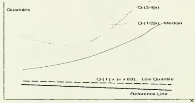
Y.

Quantiles ..••6C(3/^|x) "~

--

l^--

^—

-^

'^

0,(11X )= X b(t). LowOuanttle ReferenceLine

Figure3:

Example

4.2: Extremalconditional quantilefunctionxi->_{x P{t)} is approximately paralleltothereference linex >->_{x pr (equal to}the

mini-m£ilquantilex'P{0)in the

bounded

supportcase). Otherquantilefunctions are unrestricted, allowing for complicated forms ofglobal

heteroscedastic-ity.

The

model does not admit the reduction to a non-regression model by removing the conditional

median

(or

mean)

and/or scale from

Y

variable.

Example

4.3 Consider the

unbounded

support. For

some

referencelinex i->x'pr,

by

assumption

l(i),

P{Y

-

X'pr

<

l\X)

~

Fu{l)

=

Ti,

a.sl\

-DO,

which

implies that the paths of the extremal quantile functions

x

M- x'I3{ti) are ap-proximately parallel to that oi

x

i-^ _x'Pr- This

model

is also not "trivial" in thesense of

example

4.1, because the extremal quantiles are

determined

only

by

the extremal features ofthe conditional distribution.

As

in

example

4.2, the

model

does notrestrict

any

other features ofthedistribution,allowingforgeneral

forms

of global

heteroscedcis-ticity.

Thus

it is irreducible to a non-regression model.

Note

that

examples

4.2

and

4.3

demonstrate

that the linear location-scale

models

are neither implied

by

Model

1 nor imply

Model

1.

Thus Model

1 is ofits

own

nature, crafted to yield non-degenerate,parsimonious limits. Unlike thelocation-scalemodels,

Model

1admitsgeneral global heteroscedasticity,allowingcovariatestoaffectthe

shape

ofthe conditional distribution.

4.2

Model

2:

Congenial

Tail

Heterogeneity

We

suggest a

model

that, while flexibly accounting for the

dependence

ofthe tail

on

covariates, exhibits simplicity, enabling an explicit, practical limit theory for

both

the

extreme

and

intermediate rank

sample

regression quantiles. 13

Assumption

2

(Model

2:

Congenial

Tail

Hetrogeneity)

Suppose assumption

1

holds, except l-(i) is replaced

by

the followingtail condition:

Fy{z\x)

~

K{x)

Fu{z),

asz\-ooorz\0,

(4.12)

uniformlyin

x

£

X,

Fy, has type 1-3 tails, K{-) is

assumed

to be apositive continuous function on

X, bounded

above

and

away

from

zero,

normalized

so that

_K{fix)

=

1 (or at

any

otherreferencepoint x^ 6 X).

Just like

Model

1,

Model

2 is distribution-free, since

F^

is not

assumed

to

be

para-metric,

and

it allows the general (shape) forms of global heteroscedasticity. Unlike

Model

1,

Model

2 allows for richer effects ofcovariates

on

tails.

The

imposed

tail condition

may

seem

an

unconventional

way

to introduce het-eroscedasticity. Yet, in

many

regards, itis

more

flexible

and

constructive

than

the con-ventional location-scalemodeling,asexplained below.

The

proposed

modeling

strategy

is

motivated by

the closure of the

domains

of

minimum

attraction

under

tail equiva-lence,

and

is fully consistent withlinearity.

Indeed,

Lemma

10,characterizes this

model

in detail: (i) implicationsforthe

quan-tile coefficients ofthe linear model, (ii) limits of ratios ofspacings

between

the con-ditional quantile functions,

and

(iii)

many

other properties

needed

for inference.

Im-portantly,

we

deduced

that the linearity

assumption

and

(4.12)jointly

imply

that A'(-) can

be

represented as

{e~^

"^ _{for type 1 tails,}

{x'c)°' for type 2 tails, (4.13) {x'c)~°' for type 3 tails,

where

fi'^c

=

1 for type 2

and

3 tails,

and

/z'^c

=

for type 1 tails. In

Model

1,

c

=

for type 1 tails,

and

c

=

(1,0,...)'

=

e'j for type 2

and

3 tails.

We

call c the

tailheterogeneity index. It

measures

the strength with

which

X

shift the tails of error terms U.

Note

that x'c

>

uniformly

on

X

fortypes 2

and

3

by

assumption.

It is plausible that (potentially) the non-parametric function K{-) in (4.12) is in fact a transformation ofthe linear index x'c

determined by

the tail index ^. Recall

(,

=

(for type 1 tails)

and

£,

=

1/a

and

—

1/q

fortype 2

and

3 tails,respectively. This

assumption

leads to parsimonious, convenientlimits for regression quantiles.

The

following

examples

illustrate the model's flexibility.

Example

4.4

(Linear

Location-Scale

Model)

Assume

for

X'j

>

a.s.

Qy(r|x)

=

x'Q

+

x'7-F-'(r),

(4.14) corresponding to the location

model

Y

=

X'a

-\-X'-y

V, where

V

is

independent

of

A'^ and, say, has

mean

and

variance 1.

Assume

F^

has the extremal tail type with ^

^

0.

Then

forthe reference linex'a

and

U =

Y

—

X'a

=

X'-y-

V

P{X'-f

V

<

l\X)

~

(X'7)-^/^ -_F^il), as /

\

-co,

so the conditions of

Model

1 are satisfied with

F^

=

Fy.

The

location-scale

model

imposes two

stringent restrictions: (i) the extremal features of the distribution are

largely

determined

by

the (central)location

and

scaleparameters: /3(t)

=

a+7-F~^

(r),

and

(ii) thecovariatesare limited toaffectonly the location

and

scaleofthe conditional distribution, precluding the

shape

effects like

skewness

or kurtosis.

Example

4.5

Model

2 requires that for

some

reference line x'/J^

P{Y

-

X'pr

<

l\X)

~

K{x)

Fu{l), as/

\

or

-

cx),

which

implies that the paths of the extremal quantile functions

x

M- x'P{ti) are

no

longer parallel to that of x h-)- _x'Pr-

(The

crossing of lines is precluded because the

assumption

is consistent with linearity,

Lemma

10). This

model

is not as restrictive as

example

4.4. First, the extremal quantiles (and the reference line) are

determined

only

by

theextremal features ofthe conditional distribution. Second, the

model

allows for general global heteroscedasticity- the entire

shape

ofthe conditional density

may

change

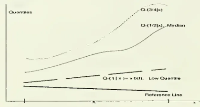
with covariates (scale, skewness, etc), including thetails.

Figure 4:

Example

4.5. Extremal quantile functions x i-> x'/3{t) are no longerapproximatelyparEilleltothereferencelinex>->_x'fir, over X, allow-ing the tail heteroscedasticity. Other quantile functions are unrestricted, allowing for complicated forms of global heteroscedasticity as well.

The

extremalfeatures ofthemodel, including thereferencelines, arenot

deter-mined

bythecentral features.

Thisdiscussion concludes the constructionofour models. In principle, itshould

be

possible to further relaxthe

modeling

assumptions, particularlyin the

nonparametric

direction, but a

good

deal of caution is

needed

to assure the joint coherency of the

tail conditions, functional

dependence

of the quantile curves

on

regressors,

and

non-degeneracy ofthe limit distributions.

Note

that the obtained

models

are coherent, flexible,distribution-free, leadtonon-degenerate,parsimoniouslimit distributions,

and

provide a convenient

framework

for inference

about

the tails.

5

Asymptotics

under

Extreme Ranks

Recall that the

approximation

concept of

extreme

ranks requires

tT —

> fc

>

0.

Here

we

state the distribution results for

Models

1

and

2

and

explain their barest essence, while leaving proofs

and

some

generalizations to the appendix.

5.1.

A

Sketch.

First, obtain a finite-dimensional {fidi)

weak

limit

Qco()

of the finite-sample, suitably scaled, objective functions {Qt{-)}-

Qoo

is defined

by

a point

processthat "counts" the "extremalevents."

Then,

the normalizedregression quantile statistic,

_{Zx, an argmin}

of

_Qt,

will convergein distribution toa

random

variable Zoo, the

argmin

of_Qoo,

by

convexity of

_{Qt]

and

Qoo-For brevity,

we

confine our discussion to type 3 tails. Consider the statistic

Zr

=

ar{P{T)-l3{0)),

where

Ct- is the canonicalscaling in section 3.6, defined in terms ofthe function F,, in

assumption

1 or 2.

Zt

optimizes therescaled

by

a^ objectivefunction in (3.4):

T

Qt{z)

=

_J2

('rPr[Ut

-

X^z/a-r)

-

a^rUt),

(5.15)

where

Ut

=

Yt

-

A'j'/?(0)

>

Q a.T\d z

=

ar{l3

-

I3r)-

We

subtracted the

"smoother"

X^j rUtCiT,

which

brings a key continuity property

and

stabilizes

Qt-

Clearlythis does notaffect the

argmin

Zr- [The

"smoother"

fortype 1-2 tails is

more

involved;

Lemma

1. Incidentally, theconventional central

rank

stabilization

by ^jPr(t/tar)

is bad, for

it sends the objective to

+00,

let alone continuity.]

Hence

T

Qt[z)

=

-TtX'z -

J2l{Utar <

X[z)

{Utar

-

X'^z). (5.16)

t=i

This function is convex. Notably, it is constructed as a continuous functional of the point process defined next.

The

fi-di distribution of

_Qt

is defined

by

that of

{Qt{zj),J

<

l] for

any

finite (z_/,j

<

/). Since A'

—

>• _/xx,

and

tT —

> k (forj

<

I) :

T

Qt{zj)

=

-kn'xZj

-

^

l{UtaT

<

XtZj)[Utar

-

X[zj)

+

Op(l). (5-17) t=i

The

limit behaviorof

_Qt

is determined

by

the pointprocess

N

that assigns

mass

to

measurable

sets

A

by:

r

N(^)

=

Y^

\{{arUt,Xt}

e A), for

AcE=

[0,oo)

x

X.

(=1

The

point process

N

is a

measure

defined

by

its

random

points (atoms) {aT.Ut,Xt,t

<

T)

(See Definition A.l, B.l).

We

find that Qt{-) is

an

integralofa residual function with respect to the point process,

which seems

to

be

special tothis problem.

Point process theory is the bread-and-butter of

extreme

value theory,^ [26],

and

is

useful here. Indeed, a Lebesgue-Stieltjes integral

_f

gdN

of

N

with points

{Xj}

is :

j

9{x)dN{x)

=

_Y^g[X,).

®Point process theorywasdevelopedbyKallenberg[44], Resnick(65] andothersinconsiderable

gen-erality. Applicationsare numerousin statistics. For example,Feigin and Resnick[29] approximatethe

constraintsofthelinearprogrammingestimators; alsoKnight[46] ;Emrechtset al.[26] andResnick[65]

show howpoint processes

may

be used inrelated applications, particularlytheexceedance processes,

extremal processes,and record values.

Convergence

of such integrals, for continuous

maps

x M- g{x} that vanish outside

compact

sets, metrizes

weak

convergence of point processes (Definition A.2.)

So

we

represent {Qt{zj),J

<

I) as an integral

Qt{zj)

=

-kn'xZj

+

[{I

-

x'zj^dNil,!)

+

Op(l), (5.18)

where

(/

—

x'z)"" is the "residual" function.

Lemma

2 proves {Qt{z),J

<

l) \s a.

continuous

map

of the point process

N,

so its

weak

limit is

determined

by

that of

N.

Notably, to obtain continuity for various tail types, the construction of point process

N

requiresacarefulchoice oftheunderlyingtopologicalspace

E

(andadditional transformationsof

_Qt

fortypes 1

and

2).

The

weak

hmit

(Def. A.2) of

N

in

Model

2 is a Poisson process

N,

Lemma

6: oo

i=l

where

{Ji,Xi] are

random

points defined as

(j„

Xi,

i>l)

^(A^'cLf

, Xi,

z>l),

Vi=£i

+...

+

£i, i

>1,

(5.19)

where

{£i} are i.i.d. exponential

random

variables with

mean

1, {Xi} are i.i.d. with law

Fx

, distributed independently of _{£i},

and

c is the tail heterogeneity parameter.

In

Model

1, becausec

=

(1,0,...), a naturalsimplification occurs:

A;'c=l,Vi.

(5.20)

The

firstresult,explainedin

Lemma

6, isnotself-evident,while (5.20)isfairlyintuitive.

Note

that N(.4)

=

_{J2i<T ^iWTU(i),X^iy} €} A),

where

[/(,) is i-th

rank

error,

and

Xu\

is

the corresponding covariate. Vector [arU^i),!

<

q)

—

> {t\''^,i

<

_q) (Section 3.6),

and

is asymptotically independent oi

Xi

by Assumption

l-(i) in

Model

1,

which

explains

the

form

of(5.19)

and

(5.20) for

Model

1. (This is nota proof).

Lemmas

5-6 provide the prooffor

Model

2 (and 1

by

implication) using the Kalenberg's theorem, Meyer's conditions,

and

a series of compositions

and

transformations of a canonical Poisson process (Def. A.4 provides a background).

We

concludethat thefidi

weak

limit of

{Qt}

is

/CX)

(jf

-

x'z)~dN{j,x)

=

-kfjLxZ

+

^(Ji

-

X[z)~

.

Therefore,

we

obtainby convexity

Lemma

1 inthe

appendix

(Theorem

5inKnight[46]) thelimit distribution for

Zt,

provided(5oo() has a unique

argmin

a.s.

and

is finite

on

an open non-empty

set (verified in

Lemma

2

and

11).

Hence

Or(/?(r)

-

_/3(0))

-^

Zoo

=

argmin

Qoo(2)- (5.21)

Finally,

Lemma

10

shows

that ax(/3(0) -/?(r)) -> fc»c in

Model

2 ( c

=

ej

=

(1,0,...)'

in

Model

1) so that

a^(4(r)-/3(r))

-k°C

+

Zn

5.2.

Results

for

Models

1

and

2.

The

above

discussion hopefully provided

an

intuitive explanation ofthe foregoingformal results for

Models

1

and

2

(Theorems

1

and

2).

The

proofs areintheappendix.

To

statetheresult,

suppose

we

have

/sequences

{Ti,i

<

1} such that t,T

—

> ki, so

we

index thenormalizedregression quantile statistic as Zriki), for

both

T

<

oo

and

T

=

oo. Define

Zrik)

=

ar (/3(t)

—

Pt

—

br^i) , fortype 1 tails,

Zrik)

=

ar (/3(r)

-

Pr) , fortype 2

&

3tails.

Also define the centered statistic

Z^{k)=ar[p{r)-P{T)).

The

canonical constants {a-j-jbr) are defined in (3.7) in

terms

offunctions F^,

which

are definedin

Assumptions

1

and

2 along with the error

term

Ut

and

Pr-The

key point process,

N()

=

_{5I(<t ^{{ariUt}

-

6t),^Y(} € )

weakly

converges (Def. A.2) to

N(

)

=

_^i>i

l{{Ji,Xt} € •)

by

Lemma

4-6, with points {Ji,Xi} defined as:

(j„

Xi, i

>

l)

=

<

(ln(rO

+

A'/c, Xi) fortype 1,

(r7^/"A7c,

Xi) for type 2,

i>l

(5.22) (rJ/^-Y/c, a;) fortype 3,

where

{Ti,i

>

1}

=

_{X!,<i^j'*

—

1}! l^j) i^

^^

i.i.d.

sequence

of unit-exponential variables;

{Xi}

is

an

i.i.d

sequence

with

law Fx-

In

Model

1, the

dependence between

Ji

and

Xi naturally disappearsin

view

of

assumption

l-(i):

X-c

=

for type 1 tails,Vz,

(5.23) -Y/c

=

1 fortype 2

&

3 tails, Vi.

Theorem

1

(Extreme

Rank

Asymptotics

in

Model

1)

Suppose

Assumption

1

and

that (a) {Yt,Xt} is

an

i.i.d. or stationary sequence, satisfying the

Meyer

conditions,

Lemma

6; (b) at least

one

component

of

X

is absolutely continuous, if

d

>

2.

Then

as

tT

-^

k,T

-^ oo, (k

=

ki,...,ki), fora.e. k

>

Zrik)

—

> Zoo{k)

=

arginf

—

kpi'^z

+

I l{u,x'

z)dN{u,x)\,

where

l{u,v)

=

l(u

<

v){v

—

u),

and

the distribution of points {Ji,

Xi]

of

N

isdefined in (5.22)-(5.23). Furthermore, {ZT{ki),i

<

l)

-^

[Z^{ki),i

<

l),

Z^{k)

^

Z'^ik)

=

Z^{k)

-

c{k),

and

[Zj-{ki),i

<

I)

—

> [Z^{ki),i

<

I),

where

c{k)

=

Ink

ei, for type 1,

—k^~ei,

for

type2,

and k=ei

, for type3 tails.