HAL Id: hal-00564746
https://hal.archives-ouvertes.fr/hal-00564746
Submitted on 9 Feb 2011
HAL is a multi-disciplinary open access
archive for the deposit and dissemination of
sci-entific research documents, whether they are
pub-lished or not. The documents may come from
L’archive ouverte pluridisciplinaire HAL, est
destinée au dépôt et à la diffusion de documents
scientifiques de niveau recherche, publiés ou non,
émanant des établissements d’enseignement et de
On electrical load tracking scheduling for a steel plant
Alain Hait, Christian Artigues
To cite this version:
Alain Hait, Christian Artigues. On electrical load tracking scheduling for a steel plant. Computers &
Chemical Engineering, Elsevier, 2011, 35 (12), pp.3044-3047. �10.1016/j.compchemeng.2011.03.006�.
�hal-00564746�
On electrical load tracking scheduling for a steel
plant
Alain Hai¨t
1and Christian Artigues
2,31
Universit´e de Toulouse, Institut Sup´erieur de l’A´eronautique et de
l’Espace
10 avenue Edouard Belin 31055 Toulouse, France
2
CNRS ; LAAS ; 7 avenue du colonel Roche, F-31077 Toulouse
Cedex 4, France
3
Universit´e de Toulouse, UPS, INSA, INP, ISAE ; UT1, UTM,
LAAS ; F-31077 Toulouse Cedex 4, France
Abstract
Nolde and Morari [10] study a steel manufacturing scheduling prob-lem where the tasks must be scheduled such that electricity consumption matches to a pre-specified periodic energy chart. They propose a contin-uous time integer linear programming formulation to solve the problem. In this note, we present an alternative continuous time formulation that improves significantly the computation time.
KeywordsSteel plant, Mixed integer linear programming, Load tracking
1
Introduction
This paper deals with production scheduling of a steel plant with energy cost. Due to demand increase and to environmental considerations, the reflexion about a better energy consumption in production is a subject of growing in-terest. New constraints and objectives challenge the classical production mod-els, from long term to short term management and from industrial networks to single plants [5, 4, 1, 6, 3].
Energy consumption is an important subject in steel plants. Electrical de-vices may induce a high power demand if the schedule is not focused on energy. Various types of energy bills exist, calculated from energy consumption, power limits and fix or time variable energy cost. Few papers have studied this aspect for steel scheduling. Boukas at al. [2] present a hierarchical approach to min-imize the makespan of a set of batches while respecting a global power limit. Nolde and Morari [10] propose a MILP scheduling model to track a pre-specified
periodic load curve. In this paper we propose an alternative model, based on [6], to solve the latter problem.
2
Problem statement
Nolde and Morari [10] study a particular steel plant called mini-mill. The lay-out is organized as an hybrid flowshop inspired from [8] where a four-step batch process transforms scrap metal into cast steel: first melting in Electrical Arc Furnaces (EAF), then Argon Oxygen Decarburization (AOD), alloying and re-finement in Ladle Furnace (LF) and finally casting in a Continuous Casting Machine (CCM). The plant is composed of two identical EAF, then one equip-ment for every other step.
A crane is used to move the batches from one equipment to another. In this model, the crane is viewed as an additional equipment. The empty dis-placements of the crane are not taken into account. Hence we will consider a seven-task process for each batch, four ”processing” tasks and three ”transporta-tion” tasks inserted between them. For each task a processing time interval is given, and no delay is allowed between the tasks. Finally, no idle time is allowed between two batches on the continuous casting machine.
The main originality of the problem comes from the objective function. The cost of a schedule depends on the overall energy consumption of the equipments, calculated on a periodic basis. A target consumption is negotiated between the electricity provider and the plant owner for every 15-minute interval. Any variation from this contracted consumption is penalized and the objective is to minimize the sum of these penalties.
Given the particular objective function, modeling the scheduling problem is not straightforward. A 15-minute discretization is not enough because of the task durations and the accuracy required to obtain good solutions. Nolde [9] proposed a discrete-time and a continuous-time model for this application. In the discrete-time model, the interval are subdivided into smaller periods for scheduling needs. The comparison has shown that the continuous-time model is more efficient. Nolde [9] claims that it is due to the high number of time points where a task may potentially start or end. It has also been shown that the computation time is linked to the wideness of task duration intervals, with refer to energy consumption intervals.
3
Continuous-time scheduling formulation
The scheduling model is given in [10]. We remind it briefly in the following. • Machines are indexed by i ∈ I, where I is the set of all machines, including
the crane. The power consumption of machine i is given by pi.
• All tasks are indexed with l ∈ L. Tasks starting and ending times are denoted ts
l and t e l.
• All jobs are indexed by k ∈ K. The tasks of a job k are given by set Lk.
• The tasks running on machine i are given by set Li.
• The task sequence is stored in the set S that contains 2-tuples with all pairs of subsequent tasks (l′, l′′) ∈ S, where task l′ precedes task l′′. The processing time of a task belongs to a predefined interval:
Tmin l ≤ t e l− t s l ≤ T max l (1)
In a sequence of tasks, the steel making process shall not be interrupted: tel′ = t
s
l′′ ∀(l′, l′′) ∈ S (2)
Given that the Electrical Arc Furnaces (first task of a job) are identical, and that the jobs are also identical, we can affirm without loss of generality that the sequence of tasks on the EAF is known. So, the cumulative constraint on the set of EAF may be converted into disjunctive constraints on each EAF. Consequently, the resource constraints of the problem are all disjunctive:
tel1 ≤ t s l2 OR t e l2 ≤ t s l1 ∀(l1, l2) ∈ L2i, i∈ I, l1< l2 (3)
A binary variable is associated to each couple (l1, l2) defined as above, and the
classical Big-M technique is used to model the disjunction. Additional binary variables δCCM
l1,l2 are used to model the working without
interruption of the continuous casting machine (CCM). tel1 6= t s l2⇒ δ CCM l1,l2 = 0 ∀(l1, l2) ∈ L 2 CCM (4) X l2∈LCCM δlCCM1,l2 = 1 ∀l1∈ LCCM (5)
4
A new task / interval overlap formulation
The objective function is based on a discretization of the time horizon at regular 15-minute intervals. The energy consumption of task l during interval n results in the multiplication of power consumption pi of the equipment used (l ∈ Li)
by the time overlap ol,n between the task and the interval. In the following,
interval n ∈ N starts at time tn−1, finishes at time tn and lasts D = tn− tn−1
constant. The beginning of the first interval is t0 = 0 and the end of the last
interval t|N | corresponds to the time horizon T .
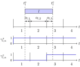
The model we propose as an alternative to that of Node and Morari [10] relies on binary variables that represent the relative position of an event and an interval. These variables are then used to model the overlaps between tasks and intervals.
t 1 2 3 4 ol,1 ol,2 ol,3 0 t γs l,n 1 1 2 3 4 0 t γe l,n 1 1 2 3 4 ts l tel l
Figure 1: Task / interval overlap and time / interval variables.
4.1
Time / interval binary variables
The following formulation, initially introduced in [11], uses binary variables to indicate wether or not an event takes place before or during an interval. Variable γs
l,n is equal to 1 if task l ∈ L begins before or during interval n, 0 otherwise
(Fig. 1).
The corresponding constraints are:
tsl ≥ tn(1 − γl,ns ) n= 1, . . . , |N | − 1 (6) tsl ≤ tn+ T (1 − γl,ns ) n= 1, . . . , |N | − 1 (7) γs l,n+1≥ γ s l,n n= 1, . . . , |N | − 1 (8) γsl,|N |= 1 (9)
In case of regular intervals of duration D, equations (6) and (7) can be written: ts l ≥ D.n(1 − γ s l,n) n= 1, . . . , |N | − 1 (10) tsl ≤ D.n + T (1 − γ s l,n) n= 1, . . . , |N | − 1 (11) Note that if ts
l exactly coincides with interval bound tn, γl,ns can either take
value 0 or 1. This is not a problem because the constraints described in the following section ensure the global consistency of time overlap determination.
4.2
Task / interval overlap
For each couple (task l, interval n), there are six possible configurations (Fig. 2) that correspond to the relative position of the task and the interval. In order to get the overlap ol,n, the type of configuration should be determined.
tn−1 tn ts te ts te ts te ts te ts te ts te (a) (b) (c) (d) (e) (f)
Figure 2: Overlap configurations of a task and an interval.
Nolde and Morari [10] use one binary variable for each configuration and ensure that only one configuration is chosen. Then they determine the appropriate overlap value. The number of binary variables is thus 6 × |N | × |L| = 6 × |N | × P
k∈K|Lk|. Moreover, the selection of the right configuration induces many
big-M constraints. Using the time / interval variables, less binary variables are needed and also less big-M constraints.
For a given task l, scheduled between ts
l and tel, the task / interval overlaps
ol,nwill only be greater than zero for the intervals where γl,ns − γl,n−1e = 1 (Fig.
1). In the same way, all the configurations can be described with time / interval variables. The following constraints give the overlaps between tasks and inter-vals according to these variables (for all task l ∈ L and interval n ∈ N , in case of regular interval of duration D):
0 ≤ ol,n≤ D(γl,ns − γ e l,n−1) (12) ol,n≥ D(γl,n−1s − γl,ne ) (13) ol,n≥ tel − D.n + D.γ s l,n−1− T .γl,ne (14) ol,n≥ D.n(1 − γl,n−1s ) − tsl − Dγ e l,n (15) X n ol,n= tel − tsl (16)
Equations (13)-(15) respectively match configurations (d), (e) and (f) while the other configurations and the global consistency are given by (12) and (16).
Given that there is no interruption between the successive tasks of a same batch, i.e. te
l = t s
l+1, the number of binary variables can be reduced: γ e l,n =
γl,n+1s . We just need to use variables γ s
l,n for the starting dates and add one
binary variable for the end of the last task of each job. Consequently, the number of binary variables is: (|N | − 1) ×P
Table 1: Power consumption of the equipments
Unit i Power consumption pi
[energy unit / min] Electric arc furnace (EAF) 1000
Crane (C) 10
Argon oxygen decarburization (AOD) 80
Ladle furnace (LF) 150
Continuous casting machine (CCM) 50
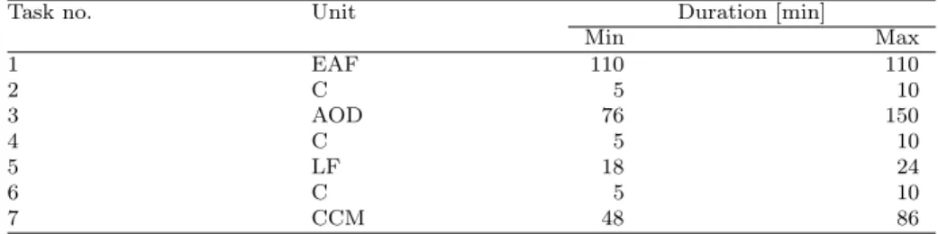
Table 2: Tasks for the production of one steel batch
Task no. Unit Duration [min]
Min Max 1 EAF 110 110 2 C 5 10 3 AOD 76 150 4 C 5 10 5 LF 18 24 6 C 5 10 7 CCM 48 86
4.3
Energy consumption by interval
The mean energy consumption of a task during an interval is given by the following constraint:
wl,n= pi.ol,n ∀i ∈ I, l ∈ Li (17)
The objective function is the sum of all tracking errors:
minX n∈N qn− X l∈L wl,n (18)
where qn is the target energy consumption for interval n.
5
Results
The example from [10] consists in scheduling 15 identical batches in order to track a given energy load curve on an horizon T = 1440 min divided into 96 intervals. Table 1 gives the power consumption of the equipments. Table 2 gives the sequence of tasks and their processing time min/max intervals.
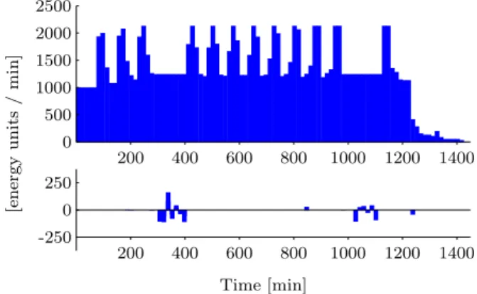
The contracted load curve, resulting from a negotiation with the energy provider, is shown in Figure 3 (top). The model is written in OPL and CPLEX 12.2 is used to solve the MILP. Tests have been performed on an Intel 2.66 GHz CPU. The new proposed formulation is solved to optimality in less than 4 min-utes. Figure 3 (bottom) presents the deviation from the target load curve. Table 3 compares the performance of the new formulation with the one of Nolde and Morari [10] obtained on a 3 GHz CPU.
200 400 600 800 1000 1200 1400 0 500 1000 1500 2000 2500 [e n er g y u n it s / m in ] Time [min] 200 400 600 800 1000 1200 1400 -250 0 250
Figure 3: Load curves: contracted load (top) and optimal deviation (bottom).
Table 3: Performance comparison
Nolde & Morari Ha¨ıt & Artigues
Constraints 233701 100465
Continuous variables 10387 10387
Binary variables 60480 13890
CPU 35 days 4 min.
Objective 1160 1037 (opt.)
6
Conclusion and future work
In this paper we propose a new continuous-time MILP formulation for the steel scheduling problem with energy constraints. This formulation turns out to be very efficient on the case study from [10]. However, the scheduling part is quite simple in this case study. It would be interesting to test the same model on more difficult problems like the steel scheduling problem from [8]. Future work will focus on decomposition approaches to solve such problems. A first application is given in [7] that present a two-level CP/MILP approach to solve parallel machine scheduling with energy costs.
References
[1] M. Agha, R. Thery, G. Hetreux, A. Ha¨ıt, and J.-M. Le Lann, Integrated production and utility system approach for optimizing industrial unit operations, Energy, 35 (2010), pp. 611–627.
[2] E. Boukas, A. Haurie, and F. Soumis, Hierarchical approach to steel production scheduling under a global energy constraint, Annals of operations research, 26 (1990), pp. 289–311.
[3] P. Castro, I. Harjunkoski, and I. Grossmann, A new continuous-time scheduling formulation for continuous plants under variable electricity
cost, Industrial & Engineering Chemistry Research, 48 (2009), pp. 6701– 6714.
[4] K.-Y. Cheung and C.-W. Hui, Total-site scheduling for better energy utilization, Journal of Cleaner Production, 12 (2004), pp. 171–184. [5] D. Gibbs and P. Deutz, Reflexion on implementing industrial ecology
through eco-industrial park development, Journal of Cleaner Production, 15 (2007), pp. 1683–1695.
[6] A. Ha¨ıt and C. Artigues, Scheduling parallel production lines with en-ergy costs, in proceedings of the 13th IFAC symposium on information
control problems in manufacturing INCOM09, Moscow, Russia, 2009. [7] , A hybrid CP/MILP method for scheduling with energy costs,
Euro-pean Journal of Industrial Engineering, to appear, (2010).
[8] I. Harjunkoski and I. Grossmann, A decomposition approach for the scheduling of a steel plant production, Computers and Chemical Engineer-ing, 25 (2001), pp. 1647–1660.
[9] K. Nolde, Optimal Control of Switched-input and Uncertain Systems, PhD thesis, ETH Zurich, Automatic Control Laboratory, 2008.
[10] K. Nolde and M. Morari, Electrical load tracking scheduling of a steel plant, Computers and Chemical Engineering, 34 (2010), pp. 1899–1903. [11] A. Pritsker and L. Watters, A zero-one programming approach to
scheduling with limited resources, Tech. Rep. RM-5561-PR, RAND Corpo-ration, 1968.