Comparison of three vertically resolved ozone data sets: climatology, trends and radiative forcings

(1)

Comparison of three vertically resolved ozone data

sets: climatology, trends and radiative forcings

The MIT Faculty has made this article openly available.

Please share

how this access benefits you. Your story matters.

Citation

Hassler, B., P. J. Young, R. W. Portmann, G. E. Bodeker, J. S. Daniel,

K. H. Rosenlof, and S. Solomon. “Comparison of three vertically

resolved ozone data sets: climatology, trends and radiative forcings.”

Atmospheric Chemistry and Physics 13, no. 11 (June 6, 2013):

5533-5550.

As Published

http://dx.doi.org/10.5194/acp-13-5533-2013

Publisher

Copernicus GmbH

Version

Final published version

Citable link

http://hdl.handle.net/1721.1/80329

Terms of Use

Creative Commons Attribution 3.0

(2)

Atmos. Chem. Phys., 13, 5533–5550, 2013 www.atmos-chem-phys.net/13/5533/2013/ doi:10.5194/acp-13-5533-2013

EGU Journal Logos (RGB)

Advances in

Geosciences

Open Access

Natural Hazards

and Earth System

Sciences

Open Access

Annales

Geophysicae

Open Access

Nonlinear Processes

in Geophysics

Open Access

Atmospheric

Chemistry

and Physics

Open Access

Atmospheric

Chemistry

and Physics

Open Access Discussions

Atmospheric

Measurement

Techniques

Open Access

Atmospheric

Measurement

Techniques

Biogeosciences

Open Access Open Access

Biogeosciences

Discussions

Climate

of the Past

Climate

of the Past

Discussions

Earth System

Dynamics

Earth System

Dynamics

Discussions

Geoscientific

Instrumentation

Methods and

Data Systems

Open Access

_{Geoscientific}

Instrumentation

Methods and

Data Systems

Geoscientific

Model Development

Geoscientific

Model Development

Discussions

Hydrology and

Earth System

Sciences

Open Access

Hydrology and

Earth System

Sciences

Ocean Science

Discussions

Solid Earth

Discussions

The Cryosphere

Natural Hazards

and Earth System

Sciences

Open Access

Discussions

Comparison of three vertically resolved ozone data sets: climatology,

trends and radiative forcings

B. Hassler1,2, P. J. Young1,2,*, R. W. Portmann2, G. E. Bodeker3, J. S. Daniel2, K. H. Rosenlof2, and S. Solomon4

1_{Cooperative Institute for Research in Environmental Sciences (CIRES), University of Colorado at Boulder, Boulder,} Colorado, USA

2_{NOAA, Earth System Research Laboratory, Chemical Sciences Division, Boulder, Colorado, USA} 3_{Bodeker Scientific, Alexandra, Central Otago, New Zealand}

4_{Department of Earth, Atmospheric, and Planetary Sciences, Massachusetts Institute of Technology, Cambridge,} Massachusetts, USA

*_{now at: Lancaster Environment Centre, Lancaster University, Lancaster, UK}

Correspondence to: B. Hassler (birgit.hassler@noaa.gov)

Received: 31 July 2012 – Published in Atmos. Chem. Phys. Discuss.: 9 October 2012 Revised: 28 March 2013 – Accepted: 4 May 2013 – Published: 6 June 2013

Abstract. Climate models that do not simulate changes in

stratospheric ozone concentrations require the prescription of ozone fields to accurately calculate UV fluxes and strato-spheric heating rates. In this study, three different global ozone time series that are available for this purpose are com-pared: the data set of Randel and Wu (2007) (RW07), Cionni et al. (2011) (SPARC), and Bodeker et al. (2013) (BDBP). All three data sets represent multiple-linear regression fits to vertically resolved ozone observations, resulting in a spa-tially and temporally continuous stratospheric ozone field covering at least the period from 1979 to 2005. The main dif-ferences among the data sets result from regression models, which use different observations and include different basis functions. The data sets are compared against ozonesonde and satellite observations to assess how the data sets repre-sent concentrations, trends and interannual variability. In the Southern Hemisphere polar region, RW07 and SPARC un-derestimate the ozone depletion in spring ozonesonde mea-surements. A piecewise linear trend regression is performed to estimate the 1979–1996 ozone decrease globally, covering a period of extreme depletion in most regions. BDBP overes-timates Arctic and tropical ozone depletion over this period relative to the available measurements, whereas the depletion is underestimated in RW07 and SPARC. While the three data sets yield ozone concentrations that are within a range of dif-ferent observations, there is a large spread in their respective ozone trends. One consequence of this is differences of al-most a factor of four in the calculated stratospheric ozone

ra-diative forcing between the data sets (RW07: −0.038 Wm−2, SPARC: −0.033 Wm−2, BDBP: −0.119 Wm−2), important in assessing the contribution of stratospheric ozone depletion to the total anthropogenic radiative forcing.

1 Introduction

Using a realistic representation of the stratospheric ozone distribution and its changes over time in a changing climate is important not only for quantifying the flux of harmful UV radiation from the sun reaching the earth’s surface, but also to understand changes in the dynamics and energy budget of the earth’s atmosphere. Capturing the observed stratospheric ozone depletion in global climate models is crucial for repro-ducing stratospheric temperature changes (Dall’Amico et al., 2010), Southern Hemisphere (SH) tropospheric circulation changes (Son et al., 2009; Polvani et al., 2011), climate and surface temperatures in Antarctica (Gillett and Thompson, 2003), global tropospheric temperature changes (Dall’Amico et al., 2009) and global precipitation changes (Purich and Son, 2012).

Global climate models that do not include interactive chemistry depend on a prescribed ozone field as input to in-corporate these effects of ozone on the climate system. The differences in modelled climate responses arising from dif-ferent input ozone fields can be significant, and can compli-cate the identification of sources of climate signal uncertainty

(3)

(e.g. Miller et al., 2006; Solomon et al., 2012). Furthermore, a data set is necessary to validate global chemistry-climate models, where ozone concentrations are calculated as part of the simulation. Therefore, a realistic ozone data set is impor-tant both for reducing the uncertainty in the climate model output, and for validation purposes.

Although many different measurement systems provide ozone measurements with high vertical resolution (multiple satellite instruments, ozonesondes, ozone lidars, etc.), no sin-gle measurement type has the temporal and spatial coverage required to create a global, zonal mean, spatially and tem-porally continuous (gap-free) stratospheric ozone data set. In particular, the tropics and the high latitudes are regions where long-term coverage is especially limited. Because a data set with incomplete coverage is not suitable as a boundary con-dition for climate models, approaches have been designed to combine different kinds of observations and to fill any re-maining gaps.

This study focuses on three ozone data sets that (i) have high vertical resolution, (ii) cover the entire globe through-out the period from at least 1979–2005, and (iii) have been mainly created to provide climate models with a realistic ozone input. All three data sets are created by using mul-tiple linear regression fits to a selected set of observations, and therefore are not identical to the original raw measure-ments. A comparison between these fitted data sets and di-rect measurements is necessary to understand their strengths and weaknesses.

This study is organised as follows. In Sect. 2, the three ozone data sets are characterized and briefly described. We consider how well the data sets capture the observed inter-annual ozone variability in Sect. 3, comparing the vertically integrated (ozone column) and vertically resolved climatolo-gies against TOMS/SBUV (Total Ozone Mapping Spectrom-eter/Solar Backscatter UltraViolet instrument) and SBUV/2 data. Section 4 discusses the climatological anomalies of the data sets. Time series from the regression-based data sets for selected months, pressure levels, and latitude zones are compared against corresponding individual data points from several measurement systems in Sect. 5. We discuss trends in the data sets in Sect. 6, focussing on the ozone change from 1979 to 1996, a period of extreme depletion in many regions. The purpose of this is to assess the extent to which the data sets capture the observed ozone decreases, although we emphasize that the data sets are not suitable for assess-ing the true ozone trend as they are all based on regression model output and any trends are effectively imposed by the fit to a linear trend or EESC basis function in the regression model. The differences in the three ozone data sets result in differences in global radiative forcing, which are discussed in Sect. 7. Finally, in Sect. 8, measures of the overall agreement between the three data sets and direct measurements from the Stratospheric Aerosol and Gas Experiment II (SAGE II) and ozonesondes are presented.

2 Brief description of the ozone data sets

Three different ozone data sets are considered in this study, all consisting of a regression model fit to observational data. The differences between the data sets arise mainly from (i) different basis functions used for the multiple linear regres-sion fit to the observations, (ii) the use of different observa-tional data to which the regression models are applied, and (iii) inclusion (or not) of the troposphere. A brief descrip-tion of each data set follows, and an overview is provided in Table 1.

2.1 Randel and Wu (RW07)

This ozone data set is described by Randel and Wu (2007). The observational data to which their regression model fit was applied are derived from SAGE I and II measurements (McCormick et al., 1989), covering ∼55◦_{S to 55}◦_{N and the}

polar regions above 30 hPa. Measurements from SAGE I are not used below 20 km. Ozonesonde data from Syowa (69◦S) and Resolute (75◦N) provide data for the polar regions from a climatological tropopause up to 30 hPa. These ozonesonde stations both lie on the edges of their respective polar vor-tices, and hence may underestimate the maximum depletion (e.g. see the comparison of Syowa and South Pole data by Solomon et al., 2005). Between 55◦S and 55◦N, the desea-sonalized data are fitted with a regression model consisting of an equivalent effective stratospheric chlorine (EESC; Daniel et al., 1995) basis function; a solar activity proxy, namely the F10.7 cm radio flux (used only above 20 km); and two or-thogonal basis functions representing the quasi-biennial os-cillation (QBO). The deseasonalized ozonesonde data are fit-ted in the polar regions only with the EESC basis function, and the regression coefficients obtained are applied at all lat-itudes poleward of 65◦. Ozonesonde trends and SAGE trends are then merged by interpolation between 55◦and 65◦. The output from the regression model therefore represents only ozone anomalies. These anomalies are then superimposed on the ozone climatology of Fortuin and Kelder (1998) (here-after FK98) to provide a global ozone data set. FK98 use ozonesonde data from 30 stations and measurements from SBUV/SBUV2 from 1980 to 1991 to create a monthly zonal mean, vertically resolved climatology. The SBUV/SBUV2 observations have a relatively low vertical resolution (about 5 km). This climatology extends from the surface to 0.3 hPa on 19 pressure levels, but the RW07 data set only uses the stratospheric levels.

RW07 spans the period from 1979 to 2005, and extends from the surface to 50km with a vertical resolution of 1 km. Since the RW07 data set is provided on an altitude grid and in ozone units of DU/km, here it has been converted onto pres-sure levels and into volume mixing ratio units (parts per mil-lion volume, ppmv) to facilitate comparisons with the other two data sets. The US standard atmosphere was used for the conversion (see the Supplement).

(4)

B. Hassler et al.: Comparison of three vertically resolved ozone data sets 5535

Table 1. Overview of the characteristics of the three different data sets and information about the basis functions (BF) included in the regression model that was used to create the data sets.

RW07 SPARC BDBP

Ozone units DU km−1 ppmv ppmv

molecules m−3

Vertical units km hPa km

hPa

Temporal resolution monthly monthly monthly

Zonal bands 90◦S–90◦N, 90◦S–90◦N, 87.5◦S–87.5◦N,

5◦zones (37) 5◦zones (37) 5◦zones (36)

Number of vertical levels 50 24 70

Highest pressure level 0.81 hPa∗ 1.0 hPa 0.046 hPa

Time period covered 01/1979–12/2005 01/1979–12/2010 01/1979–12/2006

Includes troposphere – X X Includes stratosphere X X X Linear Trend BF – – X EESC BF X X X QBO BF (2 orthog.) X – X Solar cycle BF X X X Volcano BF – – X ENSO BF – – X

∗_{if converted with the US standard atmosphere.}

2.2 SPARC

The SPARC ozone data set is described by Cionni et al. (2011) and was developed by the Atmospheric Chemistry & Climate (AC&C) initiative, a joint Stratospheric Processes and their Role in Climate (SPARC) and International Global Atmospheric Chemistry (IGAC) activity. The data set con-sists of merged chemistry-climate model and observationally based regression model output, spanning from 1850 to 2100, and was developed in support of the climate model integra-tions conducted as part of the 5th Coupled Model Intercom-parison Project (CMIP5) for the Intergovernmental Panel on Climate Change (IPCC) 5th Assessment Report (AR5) (Tay-lor et al., 2012). In this study we focus on the post 1979, observationally based part of the data set. For this period, the SPARC ozone data set is very similar to RW07, except that the QBO basis functions were omitted from the regres-sion model, which leads to less variability in the data set. As for RW07, the ozone anomalies derived from the regres-sion model are superimposed on the FK98 ozone climatology to provide complete coverage for the observationally based part of the SPARC data set. In contrast to RW07, SPARC also includes data for the troposphere, taken from chemistry-climate model simulations and merged with the stratospheric data across a climatological tropopause.

The observationally based part of the SPARC data set ex-tends from 1979 to 2009, and has a vertical range from the surface to 1 hPa on 24 pressure levels.

2.3 BDBP

The BDBP data set is fully described by Bodeker et al. (2013). The data set is based on a regression model fit to the observational ozone data from Hassler et al. (2008), incorporating measurements from SAGE I and II, the Halo-gen Occultation Experiment (HALOE) instrument, the Po-lar Ozone and Aerosol Measurement (POAM) II and III in-struments, the Limb Infrared Monitor of the Stratosphere (LIMS), the Improved Limb Array Spectrometer (ILAS and ILAS II), and over 130 ozonesonde stations globally, repre-senting substantially more data sources than used in either the RW07 or SPARC data sets. In addition, the regression model used to fit the data contains several more basis func-tions than the other data sets (see Table 1), incorporating a linear trend, EESC, the QBO (two basis functions), El Ni˜no-Southern Oscillation, the volcanic eruption of Mt Pinatubo (1991), and solar activity (F10.7 cm radio flux). Other ver-sions of the BDBP are available that use fewer basis func-tions (see Bodeker et al., 2013). The regression model is used both for determining interannual ozone variability and for de-scribing the underlying annual cycle, whereas the regression models used for the RW07 and SPARC data sets were ap-plied to deseasonalized data. Also in contrast to RW07 and SPARC, the regression model was also used to calculate gap-free ozone fields in the troposphere.

The BDBP data set extends from 1979 to 2006, and from the surface to ∼0.05 hPa (70 km) in the vertical on 70 levels spaced ∼1 km apart. BDBP is available in both a pressure and altitude coordinate system, and includes both ozone vol-ume mixing ratio and ozone number density.

(5)

34 FK98 J F M A M J J A S O N D −90 −60 −30 0 30 60 90 Latitude 5.3 5.3 6.9 6.9 8.5 8.5 SBUV J F M A M J J A S O N D −90 −60 −30 0 30 60 90 5.3 5.3 6.9 6.9 8.5 8.5 RW07 J F M A M J J A S O N D −90 −60 −30 0 30 60 90 5.3 5.3 6.9 6.9 8.5 8.5 SPARC J F M A M J J A S O N D Month −90 −60 −30 0 30 60 90 Latitude 5.3 5.3 6.9 6.9 8.5 8.5 BDBP J F M A M J J A S O N D Month −90 −60 −30 0 30 60 90 3.6 3.6 5.3 5.3 6.9 6.9 8.5 8.5 BDBP (1980−1991) J F M A M J J A S O N D Month −90 −60 −30 0 30 60 90 3.6 3.6 5.3 5.3 6.9 6.9 8.5 8.5 2 4 6 8 10 Ozone [ppmv] 1

Figure 1. Ozone climatologies at 10 hPa as a function of latitude and month, for the Fortuin & 2

Kelder climatology (FK98), a climatology derived from SBUV measurements (period 1979 to 3

2005; SBUV), for the three different data sets (RW07, SPARC and BDBP) calculated for the 4

period 1979 to 2005, and for the BDBP data set calculated for the shorter period 1980 to 1991 5

(BDBP (1980-1991)). Dark orange/brown represent high ozone values, light orange represent 6

low ozone values. 7

8

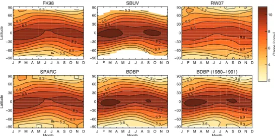
Fig. 1. Ozone climatologies at 10 hPa as a function of latitude and month, for the Fortuin & Kelder climatology (FK98), a climatology derived from SBUV measurements (period 1979 to 2005; SBUV), for the three different data sets (RW07, SPARC and BDBP) calculated for the period 1979 to 2005, and for the BDBP data set calculated for the shorter period 1980 to 1991 (BDBP (1980–1991)). Dark orange/brown represent high ozone values, light orange represent low ozone values.

3 Climatologies

3.1 Ozone at 10 hPa

For all three data sets, climatologies at key pressure levels were calculated for a common period chosen to be from 1979 to 2005. Figure 1 shows the climatologies for 10 hPa for the data sets as compared to the FK98 climatology and the ob-servations from SBUV/2 (Stolarski and Frith, 2006). Note that the SBUV data has a coarser vertical resolution than RW07 and BDBP, and the measurements registered at 10 hPa include information from pressure levels above and below 10 hPa due to the averaging kernel. In addition, Fig. 1 shows the BDBP climatology for the years 1980 to 1991, i.e. cover-ing the same period as the FK98 climatology.

The overall structure is very similar between the three data sets, the FK98 climatology and the SBUV data, notably (i) the low ozone in the tropics with a weak annual cycle maxi-mizing in February/March and again in September/October; (ii) an almost latitudinally symmetric gradient from the high tropical ozone to lower high-latitude ozone; and (iii) slightly higher values in the polar regions in late winter/early spring (Northern Hemisphere (NH): February/March; SH: Octo-ber/November).

Since both the RW07 and SPARC data sets use the ozone climatology described by FK98, their climatologies should be almost identical. While SPARC and FK98 indeed show almost an identical ozone distribution at 10 hPa, the RW07 climatology shows lower ozone than FK98 (and SPARC and BDBP) in the tropics, but similar ozone for the high lati-tudes. The differences between the RW07 and FK98 clima-tologies could be due to their different vertical resolutions. The FK98 climatology consists of 19 levels extending from

1000 hPa to 0.3 hPa, whereas the RW07 data set has 50 levels that range from the surface to about 0.8 hPa, and that were converted onto pressure levels with a standard atmosphere (see Table 1). The interpolation of the climatology onto the more highly resolved RW07 vertical levels may introduce a slight bias in the calculated pressure, with subsequent im-pacts on the conversion from DU/km to volume mixing ra-tio. In contrast, the SPARC data set has 24 levels that extend from 1000 hPa to 1 hPa, which is closer to the levels provided by the FK98 data set.

The BDBP climatology shows the highest ozone in the tropics at 10 hPa of all three data sets, closely matching the peak concentrations in the SBUV climatology. The gradient in ozone between the tropics and the mid-latitudes is steep-est for BDBP, with that data set showing the lowsteep-est 10 hPa polar ozone concentrations of all three data sets. This feature agrees well with the SBUV climatology, for the areas where data is available. The 1980–1991 BDBP climatology is sim-ilar to that calculated for 1979–2005, with slightly increased ozone concentrations due to the lower levels of ozone deplet-ing substances for 1980–1991 compared to 1979 to 2005.

Climatologies for levels lower in the atmosphere show similar patterns to the 10 hPa climatologies, with a pattern of low ozone appearing in the high-latitude spring months at levels below 50 hPa. Due to the use of the FK98 clima-tology in the construction of SPARC and RW07, differences between these data sets might be expected to be negligible. In the case of SPARC, the differences are indeed small and are likely attributable to the interpolation to different pres-sure levels and the higher resolution latitude grid. In contrast, there are more pronounced differences between the RW07 and FK98 climatologies, with ozone values being higher for RW07 from the lower stratosphere up to 50 hPa, at all

(6)

35

70°N to 90°N 1 2 3 4 5 6 7 Ozone [ppmv] 10 100 Pr es su re [h Pa ] 1 2 3 1 2 3 4 5 6 7 Ozone [ppmv] 10 100 Pr es su re [h Pa ] RW07 SPARC BDBP 1 2 3 Ozone [ppmv] 20°S to 20°N 0 2 4 6 8 10 10 100 MAM MAM 0 1 2 90°S to 70°S 7 Ozone [ppmv] Pr es su re [h Pa ] 0 1 2 3 4 5 6 10 100 0 1 2 3 Ozone [ppmv] Pr es su re [h Pa ] 100 0 1 2 3 4 5 6 7 10 100 0 1 2 3 40°N to 55°N 0 2 4 6 8 Ozone [ppmv] 10 100 0 1 2 3 0 1 2 3 0 2 4 6 8 Ozone [ppmv] 10 100 RW07 SPARC BDBP 55°S to 40°S 0 2 4 6 8 Ozone [ppmv] 10 100 4 3 2 1 0 0 2 4 6 8 10 Ozone [ppmv] 10 SON SON 0 1 2 100 0 2 4 Ozone [ppmv] 10 100 4 3 2 1 0 6 8

1 F

igure

2. Cl

im

atol

ogi

ca

l oz

one

prof

ile

s f

rom

the

thre

e oz

one

da

ta

se

ts

for

five

la

tit

ude

re

gi

ons

2 (fi

rs

t c

ol

um

n:

90°

S

to

70°

S

, s

ec

ond

col

um

n:

55°

S

to

40°

S

, thi

rd

col

um

n:

20°

S

to

20°

N

, f

ourt

h

3 col

um

n:

40°

N

to

55°

N

,

fif

th

col

um

n:

70°

N

to

90°

N

)

and

tw

o

se

as

ons

(uppe

r

row

: M

A

M

,

4 low

er

row

: S

O

N

).

T

he

low

er

stra

tos

phe

re

pa

rt

of

the

prof

ile

(100

hP

a t

o

50 hP

a,

gre

y

da

she

d

5 box) i

s e

xpa

nde

d i

n t

he

s

m

all

ins

et i

n e

ac

h gra

ph.

6

7

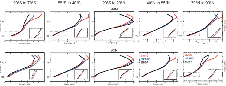
Fig. 2. Climatological ozone profiles from the three ozone data sets for five latitude regions (first column: 90◦S to 70◦S, second column: 55◦S to 40◦S, third column: 20◦S to 20◦N, fourth column: 40◦N to 55◦N, fifth column: 70◦N to 90◦N) and two seasons (upper row: MAM, lower row: SON). The lower stratosphere part of the profile (100 hPa to 50 hPa, grey dashed box) is expanded in the small inset in each graph.

latitudes. At lower pressures however, these differences van-ish almost completely.

3.2 Vertically resolved ozone

Figure 2 shows mean climatological ozone profiles for the three data sets for the Antarctic (90◦S to 70◦S), the tropics (20◦S to 20◦N), the Arctic (70◦N to 90◦N), the SH mid-latitudes (55◦_{S to 40}◦_{S), and the NH mid-latitudes (40}◦_N

to 55◦_{N), for two different seasons (MAM and SON).}

Cli-matological values are lowest for the BDBP data set in the lower stratosphere for the mid- and high latitudes. In particu-lar, there are distinctly lower ozone values over Antarctica in spring, which exist throughout the stratosphere. This might be mainly based on the fact that a logarithmic transforma-tion of the input data allows the BDBP regression model to track low ozone values well (Bodeker et al., 2013). By 50 hPa the differences between the BDBP climatology and the two other data sets become smaller. At the 30 hPa level, all three data sets climatologies are almost identical in the tropics, and BDBP is only slightly lower in the high latitudes. Between approximately 30 and 7 hPa the differences between data sets change sign in the tropics, with BDBP having higher climato-logical ozone values. However, in the polar regions, RW07 is consistently higher than BDBP, and often higher than SPARC between 30 and 7 hPa. In the tropics RW07 shows the high-est climatological values again above about 7 hPa, placing the maximum climatological ozone value clearly higher in altitude than BDBP and SPARC. Climatologies for the SH mid-latitudes show the three data sets in good agreement up to about 20 hPa, at which point the differences between them get more apparent with BDBP showing the lowest values, and RW07 showing the highest. In the NH mid-latitudes the

climatologies of SPARC and BDBP are almost identical for the whole profile, whereas RW07 is slightly higher in the lower stratosphere and from about 7 hPa upward.

These differences in climatologies throughout the strato-sphere could be caused by the different measurements used as input data for the regression models (e.g. the low ozone in Antarctic spring in BDBP). In addition, the different cov-ered time periods on which the BDBP climatology and the FK98 climatology (basis for the RW07 and SPARC clima-tologies) are based could cause some differences in climato-logical values. Furthermore, the fact that the RW07 data set had to be converted into mixing ratio units and interpolated onto pressure levels (see Sect. 2.1) might influence the pres-sure assignment. Conversion sensitivity studies (see the Sup-plement) showed that the peak height of the maximum ozone is only slightly influenced by the conversion from altitude onto pressure levels. However, the associated absolute values of the RW07 ozone profiles can differ significantly depend-ing on latitude and season, with largest differences in polar regions. The conversion chosen for the comparison shown in this study is not the exact replica of the conversion used to create the RW07 data set (combination of 7 km scale height and zonal mean, monthly mean temperature climatology (W. Randel, personal communication, 2012)); however, it puts the RW07 data on average closest to SPARC and BDBP.

4 Anomalies

Figure 3 shows the ozone column anomalies for each of the data sets, relative to their respective 1979 to 2005 climatolo-gies, together with observational data from TOMS/SBUV (Stolarski and Frith, 2006). This provides an overview of the

(7)

36 T OMS / SBUV R W07 S P ARC BDBP

Ozone column anomaly / DU

a)

b)

c)

d)

1

Figure 3. Total column ozone anomalies (with respect to 1979 to 2005) as a function of time 2

and latitude, for (a) TOMS/SBUV, and integrated ozone, from lowest to highest level 3

available, for the three datasets, (b) RW07, (c) SPARC, and (d) BDBP. White regions in (a) 4

indicate where no TOMS/SBUV data were available. Blue colours indicate negative 5

anomalies, red colours indicate positive anomalies. 6

7

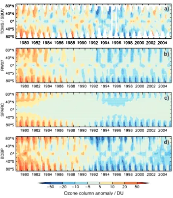
Fig. 3. Total column ozone anomalies (with respect to 1979 to 2005) as a function of time and latitude, for (a) TOMS/SBUV and inte-grated ozone from lowest to highest level available, for the three data sets, (b) RW07, (c) SPARC, and (d) BDBP. White regions in (a) indicate where no TOMS/SBUV data were available. Blue colours indicate negative anomalies, red colours indicate positive anomalies.

general ozone evolution and the degree of variability cap-tured by the three data sets. Column data for TOMS/SBUV, SPARC and BDBP all include tropospheric ozone, while this is excluded with RW07, which begins at a climatological tropopause. However, by comparing the anomalies, we re-move this systematic bias (assuming that the changes in the tropospheric burden make small contributions) and focus on interannual variability. The approach is supported by the fact that the anomalies calculated from the layered SBUV/2 data set (Bhartia et al., 2004), where ozone was integrated from approximately 64 hPa upward, show a very similar pattern to those of the TOMS/SBUV (albeit with slightly weaker posi-tive anomalies at the beginning of the time series and slightly stronger negative anomalies at the end of the time series), suggesting that tropospheric ozone only has a small influence on the total column ozone anomalies.

The TOMS/SBUV anomalies (Fig. 3a) show the well-known pattern of the ozone hole evolution in the SH po-lar region, with positive anomalies before the late 1980s and increasingly more negative anomalies thereafter. The TOMS/SBUV data are only available when the satellite can see the sun, meaning that anomalies cannot be calculated at high latitudes for all months. Figure 3a also shows that ozone depletion is apparent in the NH polar region, although not as

strong as in the SH. In the early 1990s, ozone anomalies were especially low when unusually deep NH polar ozone deple-tion was recorded (see, e.g., Newman et al., 1997). Interan-nual variability is considerable in the tropics and sub-tropics, where, in particular, the QBO signal is strong.

Figure 3b to d show that all three data sets show the de-velopment of SH ozone depletion in spring and the Antarc-tic ozone hole. The most negative anomalies at high south-ern latitudes appear in the mid-1990s, with similar magni-tudes in all data sets. In addition, all data sets show nega-tive NH anomalies in the boreal spring, but the deepest NH ozone depletion appears in the BDBP data. The presence of these more negative anomalies in the BDBP data is likely due, in part, to the volcanic basis functions: several stud-ies have linked enhanced ozone depletion to the eruption of Mt. Pinatubo (e.g. Rosenfield et al., 1997; Solomon et al., 1998; Telford et al., 2009). In addition, Bodeker et al. (2013) ascribe the distinct negative Arctic ozone anomalies during the late 1990s and early 2000s in the BDBP data set to an underestimation of the dynamically forced ozone increases, which is not tracked by the regression model due to the lack of an appropriate basis function. The BDBP more closely replicates the TOMS/SBUV NH polar temporal evolution, but its anomalies are more positive in the beginning of the time period (early 1980s), and stay more negative at the end of the time period. Overall, this results in a larger negative trend in BDBP than in SPARC, RW07 or TOMS/SBUV.

Outside of the polar regions, the impact of the inclusion of additional basis functions in the BDBP regression model is clearly apparent, with the anomalies having much more structure than in RW07 and, especially, in the SPARC data. The BDBP variability compares well to the TOMS/SBUV anomalies, suggesting that the BDBP data set is in this sense closer to reality than RW07 or SPARC. The lack of a QBO basis function in the SPARC data leads to the anomalies in the tropical and mid-latitudes having very little tempo-ral structure. Tropical ozone decreases are strongest in the BDBP data. The evolution of the tropical column ozone anomalies is well captured by the RW07. However, as for the NH polar region, tropical ozone depletion in the BDBP data set might be too strong, whereas it might be slightly too weak for SPARC. The exclusion of a (possibly changing) tropospheric column contribution could contribute to these differences.

Analysis of data set anomalies on different pressure lev-els (not shown) reveals characteristics similar to those evi-dent in the integrated ozone anomalies. Antarctic ozone de-pletion is present in RW07 up to about 50 hPa, weakening at higher altitudes. In the tropics and subtropics the RW07 anomalies are mainly characterised by a QBO pattern. As with the integrated anomalies, vertically resolved SPARC anomalies show the least variability of all three data sets. Po-lar ozone depletion and a general global tropical decreasing trend are represented, the latter being comparable in mag-nitude to RW07 for all pressure levels. The relatively low

(8)

variability for SPARC is to be expected given the smaller number of basis functions included in the fit.

As Fig. 3, the BDBP data set shows the more interannual variability than the other regression-based data sets, but it does agree reasonably well with the other data sets in the evo-lution of Antarctic anomalies. The Antarctic ozone depletion signal correlates across different pressure levels up to 10 hPa, although weakening with increasing altitude. In the Arctic, ozone depletion in the BDBP is stronger than the other two data sets. The most negative anomalies in this region appear at pressure levels up to 50 hPa in 1992/1993, following the Mt. Pinatubo eruption, but this strong anomaly disappears at higher altitudes. Negative tropical ozone anomalies are also largest for BDBP, peaking in the 2000s. In the lower strato-sphere, the tropical BDBP anomalies do not show the QBO pattern as prominently as RW07, but the QBO-signal extends further into the mid-latitudes. The BDBP QBO pattern is more clearly apparent in the mid-stratosphere and with more variability than RW07.

5 Time series

Although the comparison of the vertically integrated ozone climatologies, and anomalies of the three different data sets against TOMS/SBUV provides some validation of the three data sets, high-latitude data gaps in the TOMS/SBUV data preclude validation for those regions. For this reason, we compare the three data sets against data from several ver-tically resolved measurement systems, particularly during time of polar darkness, providing additional validation. The following four sub-sections provide a more detailed descrip-tion of the comparison of the ozone time series in the Arctic and the Antarctic, the NH mid-latitudes, and also in the trop-ics. An expanded range of these comparisons can be found in the Supplement.

We use vertical profiles from the satellite-mounted SAGE I and II, HALOE, POAM II and III instruments, and ozoneson-des from Hassler et al. (2008). These data are stored on a common vertical grid and are quality checked, but are other-wise unaltered. In addition, we use SBUV/2 monthly mean layer data (Bhartia et al., 2004), and data from the Microwave Limb Sounder (MLS) on the Upper Atmosphere Research Satellite (UARS) (Livesey et al., 2003) and the Earth Observ-ing System (EOS Aura) (Livesey et al., 2008) at pressure lev-els and latitude regions where they are available. This latter data set acts as a fully independent data source since it is not used in any of the three data sets as input for the regression models.

5.1 Northern Hemisphere polar region

Figure 4 shows the January and April time series of 80◦– 85◦N lower stratospheric ozone at four pressure levels from the three different data sets with individual measurements

37 1980 1985 1990 1995 2000 2005 Year 0 1 2 3 4 Ozone at 100 hPa [ppmv] 0 1 2 3 4 Ozone at 70 hPa [ppmv] 2 3 4 5 6 7 Ozone at 30 hPa [ppmv] January, 80°N to 85°N 2 3 4 5 6 7 8 Ozone at 10 hPa [ppmv] 1980 1985 1990 1995 2000 2005 Year April, 80°N to 85°N BDBP RW07 SPARC sondes UARS MLS AURA MLS 1

Figure 4. January (left) and April (right) ozone time series 80°N to 85°N for four different 2

pressure levels. Individual ozonesonde measurements available in this zone are shown for 3

these months (grey open circles), together with UARS MLS monthly means (dark grey, filled 4

circles) and AURA MLS monthly means (dark grey, filled stars), and the BDBP (Tier 1.4, 5

black), RW07 (red) and SPARC (blue) time series. The vertical grey line denotes the 6

inflection point selected for piecewise linear trend calculations (see Section 6). 7

8

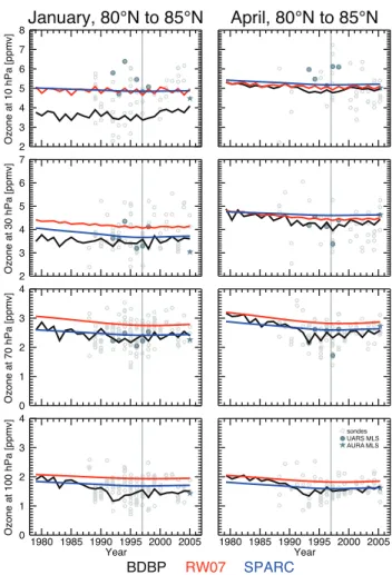
Fig. 4. January (left) and April (right) ozone time series 80◦N to 85◦N for four different pressure levels. Individual ozonesonde mea-surements available in this zone are shown for these months (grey open circles), together with UARS MLS monthly means (dark grey, filled circles) and AURA MLS monthly means (dark grey, filled stars), and the BDBP (black), RW07 (red) and SPARC (blue) time series. The vertical grey line denotes the inflection point selected for piecewise linear trend calculations (see Sect. 6).

from ozonesondes. Only ozonesonde data are shown between 80◦N and 85◦N as no satellite data are available for the com-parison in that region. All ozonesonde measurements were taken at the two Canadian sounding stations, Eureka and Alert. There are more data at the levels lower in the atmo-sphere since the altitudes reached by the ozonesonde vary between soundings.

For both January and April, the RW07 and SPARC time series are almost identical in shape at 100 and 70 hPa, al-though SPARC is consistently lower. At 30 and 10 hPa RW07 shows more variability than SPARC, due to the QBO ba-sis functions used to create this data set, and, furthermore, the offset between RW07 and SPARC becomes smaller. The BDBP time series shows the most variability at all pressure levels, with distinct QBO related features and, especially in the lower stratosphere, influences of the Mt. Pinatubo

(9)

—mboxeruption. In the lower stratosphere, the BDBP time series shows larger changes between the beginning of the time series and the mid-1990s. The overall slope of the BDBP time series is more similar to RW07 and SPARC at altitudes above 70 hPa, and the QBO-related variability dom-inates the time series structure. The BDBP time series shows lower ozone levels than RW07 at all pressure levels. Com-pared to SPARC, BDBP ozone is lower at 30 and 10 hPa, but more similar at 100 and 70 hPa. Offsets between BDBP and the other two data sets appear to depend on season, most likely due to the data set differences in climatologies (Sect. 3).

Time series of all three data sets fall within the range of the available ozonesonde measurements at all pressure levels despite their offsets, partly because the spread in the ozonesonde measurements is large. The RW07 time se-ries tends to fall on the upper end of the ozonesonde data, whereas SPARC and BDBP fall within the middle of the ozonesonde range. In the absence of soundings earlier than the late 1980s, it is difficult to judge how well the ozone de-crease in the NH polar region is represented in the three data sets. It is also unclear from this comparison which data set gives the most realistic ozone decrease as deduced from the raw measurements.

5.2 Northern Hemisphere mid-latitudes

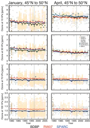
Data availability is high for the Northern Hemisphere mid-latitudes since this is a region frequently seen by satellites, and has a high density of sounding stations. Figure 5 shows the time series of ozone for the latitude band 45◦_{N to 50}◦_N

for January and April, for the three ozone data sets and measurements from SAGE I and II, HALOE, ozonesondes, SBUV/SBUV2, UARS MLS and AURA MLS.

At all four pressure levels shown RW07 is slightly higher than BDBP in January, but similar to SPARC at 30 hPa and 10 hPa. At these pressure levels, all three data sets are al-most identical in April, with the al-most pronounced difference being the higher variability in RW07 and BDBP compared to SPARC. This is due to the higher number of basis func-tions used to create these data sets. In particular, a prominent QBO-like pattern in the RW07 and BDBP can be seen from 70 hPa to 10 hPa. Overall, differences between the ozone data set time series are small, both in absolute values and in the estimated ozone decrease until the mid-1990s.

The spread in the individual measurements in winter and spring (e.g. January shown here) is high at all levels, and for all shown measurement systems, meaning that all three data set time series are well within the measurement range. Compared to January, the measurement frequency is less in April (with notably less measurements from SAGE II and HALOE), which likely contributes to the smaller variabil-ity in the measurements. Nevertheless, all three data sets are clearly within the range of the individual measurements.

38 1980 1985 1990 1995 2000 2005 Year 0.0 0.5 1.0 1.5 2.0 2.5 3.0 Ozone at 100 hPa [ppmv] 0 1 2 3 4 5 Ozone at 70 hPa [ppmv] 3 4 5 6 7 8 Ozone at 30 hPa [ppmv] January, 45°N to 50°N 4 5 6 7 8 9 10 Ozone at 10 hPa [ppmv] 1980 1985 1990 1995 2000 2005 Year April, 45°N to 50°N BDBP RW07 SPARC SAGE I SAGE II sondes HALOE UARS MLS SBUV AURA MLS 1

Figure 5. January (left) and April (right) ozone time series 45°N to 50°N for four different 2

pressure levels. Individual ozonesonde measurements available in this zone are shown for 3

these months (grey open circles), together with SAGE I and II (orange open squares), 4

HALOE (red open diamonds), and SBUV/SBUV2 (dark green, filled triangles), UARS MLS 5

monthly means (dark grey, filled circles), AURA MLS monthly means (dark grey, filled 6

stars), and the BDBP (Tier 1.4, black), RW07 (red) and SPARC (blue) time series are shown. 7

The vertical grey line denotes the inflection point selected for piecewise linear trend 8

calculations (see Section 6). 9

Fig. 5. January (left) and April (right) ozone time series 45◦N to 50◦N for four different pressure levels. Individual ozonesonde mea-surements available in this zone are shown for these months (grey open circles), together with SAGE I and II (orange open squares), HALOE (red open diamonds), and SBUV/SBUV2 (dark green, filled triangles), UARS MLS monthly means (dark grey, filled cir-cles), AURA MLS monthly means (dark grey, filled stars), and the BDBP (black), RW07 (red) and SPARC (blue) time series are shown. The vertical grey line denotes the inflection point selected for piecewise linear trend calculations (see Sect. 6).

For more mid-latitude time series comparison (Northern and Southern Hemisphere) see the Supplement.

5.3 Tropics

Figure 6 shows the tropical ozone time series between 5◦S and 5◦N for all three data sets for April and July, together with ozonesonde measurements from seven stations (Brazav-ille/Congo, Malindi/Kenya, Nairobi/Kenya, San Cristo-bal/Ecuador, Christmas Island/Australia, Sepang/Malaysia, Kaashidoo/Maldives), and measurements from SAGE I and II, HALOE, and SBUV/SBUV2. Note that no data are avail-able in April for RW07 at 100 hPa, as this is masked out by the climatological tropopause.

(10)

B. Hassler et al.: Comparison of three vertically resolved ozone data sets 5541 39 0.0 0.1 0.2 0.3 0.4 Ozone at 100 hPa [ppmv] 0.0 0.2 0.4 0.6 0.8 1.0 1.2 1.4 Ozone at 70 hPa [ppmv] 2 3 4 5 6 Ozone at 30 hPa [ppmv] 6 7 8 9 10 11 12 Ozone at 10 hPa [ppmv] 1980 1985 1990 1995 2000 2005 Year April, 5°S to 5°N 1980 1985 1990 1995 2000 2005 Year July, 5°S to 5°N BDBP RW07 SPARC SAGE I SAGE II sondes HALOE UARS MLS SBUV AURA MLS 1

Figure 6. April (left) and July (right) ozone time series between 5°S to 5°N for four different 2

pressure levels. Individual ozonesonde (grey open circles), SAGE I and II (orange open 3

squares), HALOE (red open diamonds), and SBUV/SBUV2 (dark green, filled triangles), 4

UARS MLS monthly means (dark grey, filled circles), AURA MLS monthly means (dark 5

grey, filled stars), and the BDBP (Tier 1.4, black), RW07 (red) and SPARC (blue) time series 6

are shown. The vertical grey line denotes the inflection point selected for piecewise linear 7

trend calculations. 8

9

Fig. 6. April (left) and July (right) ozone time series between 5◦S

to 5◦N for four different pressure levels. Individual ozonesonde

(grey open circles), SAGE I and II (orange open squares), HALOE (red open diamonds), and SBUV/SBUV2 (dark green, filled trian-gles), UARS MLS monthly means (dark grey, filled circles), AURA MLS monthly means (dark grey, filled stars), and the BDBP (black), RW07 (red) and SPARC (blue) time series are shown. The vertical grey line denotes the inflection point selected for piecewise linear trend calculations.

For 100 and 70 hPa, values from the SPARC time se-ries are bracketed by higher RW07 and lower BDBP values at the pressure levels shown. At 100 hPa in July, RW07 is around 60 % higher than SPARC, and 60 % to 100 % higher than BDBP. At 70 hPa, RW07 is only slightly higher than both BDBP and SPARC, but at 30 hPa the three data sets are almost identical. The lack of a QBO basis function re-duces the interannual variability in the SPARC time series, whereas both RW07 and BDBP show a strong QBO related pattern at 30 hPa, which is even more pronounced in RW07 at 10 hPa. In contrast to the 100 hPa and 70 hPa, the RW07 time series is lower than the other two data sets at 10 hPa. For April at 10 hPa, the difference between the RW07 and SPARC time series ranges from 0.5 ppmv to 1 ppmv, and be-tween the RW07 and BDBP is at least 1 ppmv for all years. While all three data sets show minimal ozone decreases with

40 0.01 0.10 1.00 10.00 Ozone at 100 hPa [ppmv] 0.01 0.10 1.00 10.00 Ozone at 70 hPa [ppmv] 0 1 2 3 4 5 Ozone at 30 hPa [ppmv] 2 3 4 5 6 7 8 Ozone at 10 hPa [ppmv] 1980 1985 1990 1995 2000 2005 Year

October, 90°S to 85°S

BDBP RW07 SPARC POAM sondes 1

Figure 7. October ozone time between 85°S and 90°S for four different pressure levels. 2

Individual ozonesonde (grey open circles), and POAM II and III (violet starts), and the BDBP 3

(Tier 1.4, black), RW07 (red) and SPARC (blue) time series are shown. The vertical grey line 4

denotes the inflection point selected for piecewise linear trend calculations. 5

6

Fig. 7. October ozone time between 85◦S and 90◦S for four

dif-ferent pressure levels. Individual ozonesonde (grey open circles), and POAM II and III (violet starts), and the BDBP (black), RW07 (red) and SPARC (blue) time series are shown. The vertical grey line denotes the inflection point selected for piecewise linear trend calculations.

time at the 30 hPa and 10 hPa levels, at 70 hPa and 100 hPa a clear decrease in ozone is present in the BDBP time series from the beginning of the time series until the late 1990s (as described in Sect. 4).

Figure 6 also shows that the spread between measurements from the different data sources, and even between measure-ments from the same data source, can be large between 5◦S and 5◦N. In particular, there is a step-function type differ-ence between SAGE I (1979–1981) and later measurements. At 100 hPa in July, RW07 ozone is substantially higher than all the measurements except SAGE I values, SPARC falls in the higher range of the measurements, whereas BDBP

(11)

values are consistent with the data from the other sources. At the lowest pressure level (10 hPa), the BDBP time se-ries tracks the ozone values from the bulk of the measure-ments, whereas SPARC, and especially RW07, are at the lower range. While ozone decreases during the first 15 to 20 yr of the period appear to be present in the measurements (e.g. July at 70 hPa), this decrease is linked to the ozone values provided by SAGE I at the very start of the period. Since the measurements are highly variable for the different months and over the analysed pressure range (see figures in the Supplement), the validity of this ozone depletion in the BDBP time series cannot be confirmed. On the other hand, the lack of ozone depletion in RW07 and SPARC also cannot be confirmed (Solomon et al., 2012).

5.4 Southern Hemisphere polar region

Figure 7 shows October ozone mixing ratios for the three data sets at 100, 70, 30 and 10 hPa for the latitude zone 85◦S–90◦S, together with ozonesonde data from the South Pole station (the only station in this latitude band) and mea-surements from both POAM instruments, which are avail-able from the mid-1990s onward. This time and location was chosen for comparison to examine the maximum depletion in the Antarctic ozone hole (e.g. Solomon, 1999). Note that the graphs for 100 hPa and 70 hPa are displayed with a log-arithmic y-axis to show the severe depletions that are often measured within the ozone hole.

RW07 and SPARC time series for 100 hPa and 30 hPa are similar, with a strong ozone decrease through the late 1990s. At 10 hPa SPARC is offset from RW07 and BDBP by about 1 ppmv. There is a QBO-like pattern in RW07, and there is no trend in SPARC, differing significantly from the other layers shown. The SPARC time series for 70 hPa is some-what unusual since it follows RW07 closely until the early 1990s and then drops to much lower values in the late 1990s. This is the atmospheric region of highest ozone depletion in Antarctic spring (e.g. Solomon et al., 2005) and a realistic representation of the degree of ozone depletion is important for climate change attribution studies with climate models, a task for which all three data sets are intended. BDBP shows a distinctly stronger and earlier ozone decrease than RW07 and SPARC at 100 hPa and 70 hPa, but a similar trend at 30 hPa and 10 hPa. BDBP is offset from the two other data sets by up to approximately 1.5 ppmv at 30 and 10 hPa, but all three data sets start at approximately the same 1979 values at 100 hPa and 70 hPa. BDBP appears to agree better with the South Pole observations, which is not surprising since this is the only data set to incorporate those data; both RW07 and SPARC only use observations from Syowa station at 69◦S. As ozone abundances reach lower values in the heart of the south polar vortex, this also explains why the ozone depletion is strongest with BDBP.

South Pole ozonesonde measurements show a clear de-crease in ozone after the mid-1980s, with lowest values in

the late 1990s/early 2000s, between 100 hPa and 30 hPa. Al-though no electrochemical sonde data are available at the South Pole prior to 1986, Solomon et al. (2005) showed that earlier measurements there from the Brewer system also sup-port a strong decline in ozone in the 1980s. The BDBP time series capture the decrease at the three lower levels, and are centred in the measurement spread. While the RW07 and SPARC underestimate the ozone depletion described by the measurements, the sharp decrease in SPARC at 70 hPa from the early to late 1990s shifts that time series closer to the cen-tre of the measurement spread. At 10 hPa, the spread in the measurements is large, encompassing the time series of all three data sets. SPARC lies at the higher end of the measure-ments, RW07 is lower than SPARC but still at the higher end of the measurements, and BDBP closer to the centre.

6 Trends

All three data sets that are part of this comparison are gen-erated using multiple linear regression methods. Any ozone trends in these data sets are effectively imposed by their EESC basis function fit to the underlying measurements. Therefore, the purpose of the trends calculated in this section is to evaluate the differences between the three data sets, and to serve as reality-check when compared to trends derived directly from measurement time series.

We applied a multiple linear regression model to all three data sets, which was similar to that used to construct the three data sets, but replacing the EESC basis function with two piecewise linear trends (Reinsel et al., 2002). The inflec-tion point, i.e. the time when the second trend term of the piecewise linear trend method is allowed to deviate from the first trend term, was set at the end of 1996, as suggested by Reinsel et al. (2002). This approach has also been applied to describe ozone depletion up to the peak of anthropogenic chlorine and bromine concentrations in the stratosphere (e.g. Newchurch et al., 2003; Steinbrecht et al., 2006; Jones et al., 2009). In addition to the two trend terms, the regression model included an offset term (to describe the average an-nual ozone amount) and basis functions to describe ozone variability due to the QBO, solar cycle and ENSO. Autocor-relation in the residuals of the regression model was consid-ered (Bodeker et al., 1998). We focus our discussion on the results for the first trend term, describing the ozone change from the beginning of 1979 to the end of 1996, in the follow-ing sections.

6.1 Annual mean trends

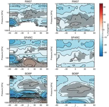
Figure 8 shows the annual mean trends calculated from all three data sets for the period 1979 through 1996 as a func-tion of latitude and pressure. This comparison focuses on the stratosphere, as the tropospheric trends are not statistically significantly different from zero for the analysed time period.

(12)

Annual mean ozone trends displayed as a function of lat-itude and pressure or altlat-itude show a distinct pattern: strong ozone depletion in the high-latitude lower stratosphere, with stronger trends in the SH than the NH (as suggested by to-tal column ozone trends, e.g. WMO, 1999, Fig. 4-18; Randel and Wu, 2007), a weaker ozone decrease in the tropics, and a region in the middle stratosphere where trends are not sta-tistically significantly different from zero (e.g. WMO, 1999, Fig. 4-32; Randel and Wu, 2007; McLinden et al., 2009). In the upper stratosphere between 40 km and 50 km (4 hPa to 1 hPa) a stronger ozone decrease occurs again, especially in the high latitudes of both hemispheres (e.g. McLinden et al., 2009). These general features are all reproduced by all three data sets, although some differences exist. The polar lower stratosphere trends in RW07 and SPARC are very sim-ilar in structure and amplitude, and both show lower trends in the Arctic compared to the Antarctic. The maximum ampli-tude of the ozone depletion in Antarctica is slightly greater in RW07 than in SPARC. The BDBP shows larger ozone de-creases at the highest latitudes near 100 hPa to 70 hPa in both polar regions, while the changes for RW07 and SPARC are constant in latitude poleward of the Syowa (69◦S) and Res-olute (75◦N) ozonesonde stations, the two stations used as raw input for the polar regions in the RW07 and SPARC re-gression models.

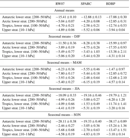
Table 2 summarizes the mean decadal trends for differ-ent regions of the stratosphere for all three data sets. Differ-ences in annual mean trends between RW07 and SPARC in the Antarctic lower stratosphere are about 2–3 % per decade. Trends for BDBP in this region are only slightly larger than RW07 (approx. 2 % more ozone decrease per decade); how-ever, strong negative trends in BDBP extend into the mid-dle stratosphere and farther into the mid-latitudes. Trends in the Arctic lower stratosphere from BDBP are much stronger than either RW07 or SPARC. Such a trend magnitude is not supported by total column ozone trend analyses (e.g. WMO, 1999, Fig. 4-18; Randel and Wu, 2007) and most likely is an artefact of the methods used in creating of the BDBP data set. Individual raw measurements in the Arctic (see Fig. 4) show a wide spread amongst measurements during the same month; however, a decrease in ozone over the years appears to exist in that latitude zone at least for the lower strato-spheric pressure levels. The magnitude of this decrease in the BDBP data set is mainly determined by two factors: (1) the lack of measurements available at the beginning of the time series in this latitude zone, and (2) the presence of unusually low ozone values at the end of the fitting period (mid-1990s; WMO, 2003, Figs. 3-30 and 3-31); e.g. see the time series for 70 hPa in April in Fig. 6. With no data to anchor the trend at the beginning of the time series, the method used to create the BDBP data set (Bodeker et al., 2013) likely overestimates the ozone decrease in the Arctic lower stratosphere.

The annual mean trends in the tropical lower stratosphere also differ considerably amongst the three data sets. Trends derived from RW07 and SPARC are similar, although they

41 RW07 −90 −60 −30 0 30 60 90 1000 100 10 1 Pressure [hPa] −7.5 −7.5 −5.0 −5.0 −5.0 −5.0 −5.0 −2.5 −2.5 −2.5 0.0 0.0 0.0 RW07 −60 −30 0 30 60 10 1 Pressure [hPa] −5.0 −5.0 −5.0 −2.5 −2.5 0.0 SPARC −90 −60 −30 0 30 60 90 1000 100 10 1 Pressure [hPa] −7.5 −7.5 −7.5 −5.0 −5.0 −5.0 −2.5 −2.5 0.0 0.0 2.5 5.0 SPARC −60 −30 0 30 60 10 1 Pressure [hPa] −7.5 −7.5 −5.0 −2.5 −2.5 0.0 BDBP −90 −60 −30 0 30 60 90 Latitude 1000 100 10 1 Pressure [hPa] −15.−10.0₀ −7.5 −7.5 −5.0 −5.0 −5.0 −5.0 −5.0 −2.5 −2.5 0.0 0.0 0.0 2.5 2.5 2.5 5.0 5.0 7.510.0 −30 −20 −10 0 10 20 30 % change/dec BDBP −60 −30 0 30 60 Latitude 10 1 Pressure [hPa] −10.0 −7.5 −5.0 −5.0 −5.0 −2.5 0.0 1

Figure 8. Left column: Annual mean trend [% per decade] as a function of latitude and 2

pressure for the time period 1979 to 1996, for the RW07 dataset, for the SPARC dataset, and 3

the BDBP dataset. Hatched regions show trends that are not significantly different from zero 4

at the 2! level. Blue colours indicate negative trends, red colours indicate positive trends. 5

Contour levels are: ±35, ±30, ±25, ±20, ±15, ±10, ±7.5, ±5, ±2.5, 0. Right column: same as 6

left column, but enlarged to the region 60°S to 60°N, 70 hPa to 1 hPa. Note that no trend 7

values are available for RW07 in the troposphere since RW07 is only defined in the 8

stratosphere. 9

10

Fig. 8. Left column: Annual mean trend (% per decade) as a func-tion of latitude and pressure for the time period 1979 to 1996, for the RW07 data set, for the SPARC data set, and the BDBP data set. Hatched regions show trends that are not significantly different from zero at the 2σ level. Blue colours indicate negative trends, red colours indicate positive trends. Contour levels are ±35, ±30, ±25,

±20, ±15, ±10, ±7.5, ±5, ±2.5, 0. Right column: same as left

column, but enlarged to the region 60◦S to 60◦N, 70 hPa to 1 hPa. Note that no trend values are available for RW07 in the troposphere since RW07 is only defined in the stratosphere.

are slightly larger for RW07 (Fig. 8 left column and Ta-ble 2). BDBP trends are two to four times larger in that re-gion. Forster et al. (2007) calculated tropical lower strato-spheric ozone trends from SAGE II measurements between 1984 and 2005. While the trend pattern they obtained appears similar to the pattern shown for the BDBP trends (Forster et al., 2007), the magnitude of their trends is approximately −5 % to −7 % per decade. This is more similar to the range of the trends from RW07, but somewhat larger than the SPARC trends. Furthermore, Randel and Thompson (2011) combined SAGE II ozone measurements from 20◦S to 20◦N with tropical ozonesonde measurements for the period from 1984 and 2009 and estimated an ozone decrease of approxi-mately −4 % per decade between 1984 and 2009 at ∼70 hPa. This too is closer to trends derived from RW07 and SPARC than to BDBP.

The comparisons suggest that it may be the inclusion of SAGE I data in the BDBP data set that is creating the anomalously large ozone trends in BDBP. However, trends shown in Fig. 8 and Table 2 describe the ozone changes from 1979 to 1996, covering a different time pe-riod than either Forster et al. (2007) or Randel and Thomp-son (2011). Trends from these studies are therefore not

(13)

Table 2. Annual and seasonal mean ozone trends and their 1σ uncertainty for the three different data sets for four different atmospheric

regions. Trends are given % per decade and are calculated for the time period 1979 to 1996. Antarctic region: 90◦S to 70◦S; Arctic

region: 70◦N to 90◦N; tropics: 20◦S to 20◦N. DJF: December-January-February; MAM: March-April-May; JJA: June-July-August; SON:

September-October-November.

RW07 SPARC BDBP

Annual means

Antarctic lower strat. [200–50 hPa] −15.41 ± 0.10 −12.88 ± 0.13 −17.88 ± 0.30

Arctic lower strat. [200–50 hPa] −5.04 ± 0.07 −4.20 ± 0.08 −12.85 ± 0.31

Tropics, lower strat. [100–50 hPa] −4.70 ± 0.21 −2.58 ± 0.21 −12.74 ± 0.53

Upper strat. [10–1 hPa] −4.89 ± 0.06 −5.52 ± 0.06 −3.94 ± 0.04

Seasonal means – DJF

Upper strat. [10–1 hPa] −5.06 ± 0.20 −5.44 ± 0.20 −4.31 ± 0.14

Seasonal means – MAM

Upper strat. [10–1 hPa] −5.40 ± 0.27 −6.15 ± 0.19 −4.57 ± 0.14

Seasonal means – JJA

Upper strat. [10–1 hPa] −4.41 ± 0.19 −5.31 ± 0.19 −3.20 ± 0.16

Seasonal means – SON

Upper strat. [10–1 hPa] −4.58 ± 0.19 −4.83 ± 0.19 −3.10 ± 0.14

necessarily directly comparable to the trends derived here. When the Forster et al. (2007) methodology is applied to the three data sets and linear trends calculated for the same time period (1984 to 2005), the trends derived from BDBP range from around −7 % to −8 % per decade in the tropical lower stratosphere, compared to around −3 % per decade for RW07 and around −2 % per decade for SPARC. BDBP trends then are similar to the trends reported by Forster et al. (2007), whereas RW07 and SPARC trends are clearly smaller.

Several studies show only annual mean trends between 60◦S and 60◦N, from around 70 hPa up to around 1 hPa (e.g. Wang et al., 2002; McLinden et al., 2009; WMO, 2011, Fig. 2-4). This is the region of the stratosphere that is well covered by SAGE II measurements, and therefore trend cal-culations are rather straightforward there. Figure 8 (right col-umn) shows the annual mean trends calculated from the three data sets, displayed for the same geographical and atmo-spheric region as the SAGE data. Trends at around 70 hPa for RW07 are only slightly larger than for SPARC, and both

agree well with trends derived from SAGE I/II by Wang et al. (2002). This is expected since both RW07 and SPARC are heavily based on SAGE data in this region. BDBP trends in this region can be more than double these values, espe-cially in the tropics, which is likely due to additional data sources being used for the creation of the data set and the more complex regression method.

Another region of special interest for annual mean ozone trends is the upper stratosphere where a response to climate change (e.g. increasing greenhouse gas concentrations) is ex-pected in addition to the impact of changes in ozone deplet-ing substances. Upper stratospheric trends for all three data sets strengthen with increasing latitude, but are weaker than in the lower stratosphere (Fig. 8, left column). The magni-tudes of the trends for the three data sets are similar, with BDBP showing a slightly weaker annual mean ozone de-crease (ca. −4 % per decade) than RW07 (ca. −5 % decade) and SPARC (ca. −5.5 % per decade; Table 2). A small area of positive trends in the Antarctic in the BDBP data set, around

(14)

2 hPa, does not likely represent a real ozone increase from 1979 to 1997, but is more likely caused by constraining errors of the BDBP regression method, as described by Bodeker et al. (2013). Overall, SPARC trends are slightly more negative than RW07 and BDBP in the tropics and mid-latitudes in the upper stratosphere. They are strongest in the SH polar region, poleward of 60◦S, and between 4 hPa and 1 hPa (see Cionni et al., 2011). This pattern does not appear in RW07 or BDBP. SAGE data alone show trends in the upper stratospheric region up to −8 % per decade (McLinden et al., 2009) and slightly higher (Wang et al., 2002), with a very similar spa-tial pattern to the trend for the data sets. SPARC is the data set with trends closest to the SAGE trends. Trends derived by analysing only SBUV data, as shown in McLinden et al. (2009), are slightly lower (up to −6 % per decade) and are therefore closer to the trends derived from RW07 and BDBP.

6.2 Seasonal trends

Table 2 shows seasonal trends and their statistical uncertain-ties for the three different data sets. All calculated seasonal trends are statistically significant at the 2σ level, except the MAM trend for BDBP in the SH polar lower stratosphere. Uncertainties are up to three times higher for the BDBP trends than for RW07 and SPARC, owing to the higher vari-ability in this data set. The uncertainties presented in Table 2 show that the three data sets seldom overlap within their re-spective statistical errors, and it is structural uncertainties that dominate the differences between them. Nevertheless, it is useful to examine the seasonality of the statistical uncertain-ties.

Differences between the data sets are most pronounced for the tropical lower stratosphere, where BDBP trends are up to three times higher than RW07 and SPARC trends in all seasons (Solomon et al., 2012), although trends differ only slightly between the seasons for a given data set. Trends in the upper stratosphere also do not differ much for the differ-ent seasons, and the three differdiffer-ent data sets are ranked in the same pattern for all seasons: BDBP shows the smallest trend, followed by RW07 and SPARC with the largest trends. In JJA BDBP trends are up to 40 % smaller than those of SPARC; RW07 trends are up to 15 % smaller than SPARC.

The largest seasonal difference in trends is present for the SH polar lower stratosphere. For BDBP, the trends are not significant in MAM and are approximately −38 % per decade in SON. Seasonal variability in trends for this region is not as high for RW07 and SPARC; however, both these data sets are similar with their smallest trends in MAM and their largest trends in SON. Trends for RW07 are larger than for SPARC (except JJA), and trends for BDBP are stronger than for RW07 (except MAM). Differences are largest in Antarctic spring (SON) when most ozone depletion happens: trends for BDBP are approximately 35 % higher than RW07 trends, and twice as large as SPARC trends.

Trends in the NH polar lower stratosphere are largest in all seasons for BDBP, and are of comparable magnitude for RW07 and SPARC. Differences between BDBP and the other two data sets can reach up to four times the trend value (e.g. in DJF), and are only of comparable magnitude for JJA. Sea-sonal differences are largest for BDBP, ranging from -18% per decade in DJF to −6 % per decade in JJA. The weakest seasonal cycle in trends is found for SPARC, where trends range from −4.8 % per decade in DJF to 3 % per decade in JJA.

7 Radiative forcing

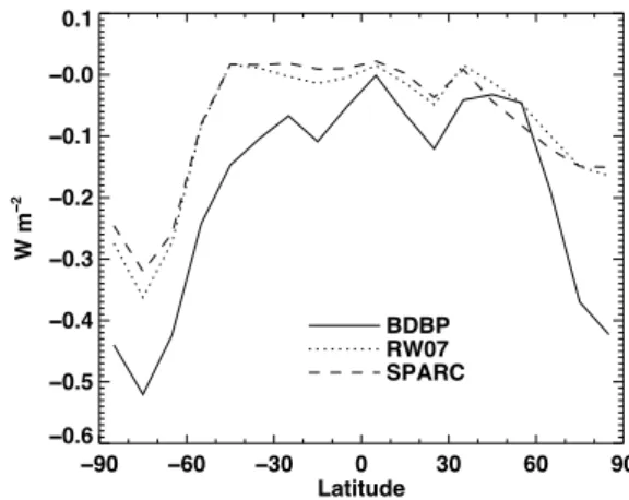
In this section, we compare the ozone radiative forcing im-plied by the three data sets. The ozone radiative forcing is defined as the net change in radiation entering the tropo-sphere due to a change in ozone. The adjusted radiative forc-ing was computed, which is where stratospheric temperatures are adjusted to the ozone changes using the fixed dynamical heating approximation. This adjustment is a first order effect for stratospheric ozone changes, whereas for other forcing agents it is typically only a 10–20 % effect.

The radiative forcing for stratospheric ozone changes is examined over the period of maximum ozone depletion, us-ing averages of 1979–1981 for the background state and 1995–1997 for the heavily depleted period. Data from the In-ternational Satellite Cloud Climatology Project (ISCCP) are used for the temperature and cloud fields and the calculation is done using seasonal averages. This radiative forcing code is the same as used by Portmann et al. (2007), which has been shown to compare well with other codes (Forster et al., 2005).

Table 3 shows the computed radiative forcing values. Tro-pospheric ozone changes are not included because they are relatively small during this time period and because one of the data sets (RW07) does not include tropospheric ozone. The table shows the large cancellation between the instanta-neous forcing and the stratospheric adjustment, which makes the accurate calculation of the total forcing sensitive to small differences. The uncertainty in the total radiative forcing is proportional to the instantaneous and adjustment values, meaning that even a modest 10 % uncertainty in these val-ues translates to a 0.03 Wm−2uncertainty in the total forc-ing. The BDBP data set induces considerably more radia-tive forcing than RW07 or SPARC data sets. This is a con-sequence of larger ozone decreases in the subtropics in both hemispheres and the SH mid-latitudes (see Fig. 9). The dif-ferences in radiative forcing between the ozone data sets im-ply different surface climate responses when the ozone data sets are used in climate models; further, the larger ozone de-creases at mid- and high latitudes in the BDBP data set can be expected to cause larger responses of climatic modes of variability (e.g., the SAM and NAM) compared with RW07 and SPARC data sets.