HAL Id: cea-01270924
https://hal-cea.archives-ouvertes.fr/cea-01270924
Submitted on 8 Feb 2016
HAL is a multi-disciplinary open access
archive for the deposit and dissemination of
sci-entific research documents, whether they are
pub-lished or not. The documents may come from
teaching and research institutions in France or
abroad, or from public or private research centers.
L’archive ouverte pluridisciplinaire HAL, est
destinée au dépôt et à la diffusion de documents
scientifiques de niveau recherche, publiés ou non,
émanant des établissements d’enseignement et de
recherche français ou étrangers, des laboratoires
publics ou privés.
Energy-resolved X-ray variability 1999–2011
V. Grinberg, K. Pottschmidt, M. Böck, C. Schmid, M. A. Nowak, P. Uttley, J.
A. Tomsick, J. Rodriguez, N. Hell, A. Markowitz, et al.
To cite this version:
V. Grinberg, K. Pottschmidt, M. Böck, C. Schmid, M. A. Nowak, et al.. Long term variability of
Cygnus X-1 - VI. Energy-resolved X-ray variability 1999–2011. Astronomy and Astrophysics - A&A,
EDP Sciences, 2014, 565, pp.A1. �10.1051/0004-6361/201322969�. �cea-01270924�
A&A 565, A1 (2014) DOI:10.1051/0004-6361/201322969 c ESO 2014
Astronomy
&
Astrophysics
Long term variability of Cygnus X-1
?
VI. Energy-resolved X-ray variability 1999–2011
V. Grinberg
1,2, K. Pottschmidt
3,4, M. Böck
5, C. Schmid
1, M. A. Nowak
2, P. Uttley
6, J. A. Tomsick
7, J. Rodriguez
8,
N. Hell
1,9, A. Markowitz
1,10,11, A. Bodaghee
7, M. Cadolle Bel
12, R. E. Rothschild
10, and J. Wilms
11 Dr. Karl-Remeis-Sternwarte and Erlangen Centre for Astroparticle Physics (ECAP), Friedrich Alexander Universität
Erlangen-Nürnberg, Sternwartstr. 7, 96049 Bamberg, Germany e-mail: victoria.grinberg@fau.de
2 Massachusetts Institute of Technology, Kavli Institute for Astrophysics, Cambridge MA 02139, USA 3 CRESST, University of Maryland Baltimore County, 1000 Hilltop Circle, Baltimore MD 21250, USA 4 NASA Goddard Space Flight Center, Astrophysics Science Division, Code 661, Greenbelt MD 20771, USA 5 Max-Planck-Institut für Radioastronomie, auf dem Hügel 69, 53121 Bonn, Germany
6 Astronomical Institute “Anton Pannekoek”, University of Amsterdam, Kruislaan 403, 1098 SJ Amsterdam, The Netherlands 7 Space Sciences Laboratory, 7 Gauss Way, University of California, Berkeley CA 94720, USA
8 Laboratoire AIM, UMR 7158, CEA/DSM – CNRS – Université Paris Diderot, IRFU/SAp, 91191 Gif-sur-Yvette, France 9 Lawrence Livermore National Laboratory, 7000 East Ave., Livermore CA 94550, USA
10 Center for Astrophysics and Space Sciences, University of California San Diego, La Jolla, 9500 Gilman Drive, CA 92093, USA 11 Alexander von Humboldt fellow
12 Ludwig-Maximilians University, Excellence Cluster “Universe”, Boltzmannstr. 2, 85748 Garching, Germany
Received 1 November 2013/ Accepted 16 February 2014
ABSTRACT
We present the most extensive analysis of Fourier-based X-ray timing properties of the black hole binary Cygnus X-1 to date, based on 12 years of bi-weekly monitoring with RXTE from 1999 to 2011. Our aim is a comprehensive study of timing behavior across all spectral states, including the elusive transitions and extreme hard and soft states. We discuss the dependence of the timing properties on spectral shape and photon energy, and study correlations between Fourier-frequency dependent coherence and time lags with features in the power spectra. Our main results follow. (a) The fractional rms in the 0.125–256 Hz range in different spectral states shows complex behavior that depends on the energy range considered. It reaches its maximum not in the hard state, but in the soft state in the Comptonized tail above 10 keV. (b) The shape of power spectra in hard and intermediate states and the normalization in the soft state are strongly energy-dependent in the 2.1–15 keV range. This emphasizes the need for an energy-dependent treatment of power spectra and a careful consideration of energy- and mass-scaling when comparing the variability of different source types, e.g., black hole binaries and AGN. PSDs during extremely hard and extremely soft states can be easily confused for energies above ∼5 keV in the 0.125–256 Hz range. (c) The coherence between energy bands drops during transitions from the intermediate into the soft state but recovers in the soft state. (d) The time lag spectra in soft and intermediate states show distinct features at frequencies related to the frequencies of the main variability components seen in the power spectra and show the same shift to higher frequencies as the source softens. Our results constitute a template for other sources and for physical models for the origin of the X-ray variability. In particular, we discuss how the timing properties of Cyg X-1 can be used to assess the evolution of variability with spectral shape in other black hole binaries. Our results suggest that none of the available theoretical models can explain the full complexity of X-ray timing behavior of Cyg X-1, although several ansatzes with different physical assumptions are promising.
Key words.X-rays: binaries – stars: individual: Cygnus X-1 – binaries: close
1. Introduction
The canonical states of accreting black hole binaries have first been observed and defined in the spectral domain: a hard state with a power law spectrum with a photon spectral index of ∼1.7 and a soft state with a spectrum dominated by thermal emission from an accretion disk. They are joined by usually short-lived transitional or intermediate states. The whole sequence of states – from hard state over the intermediate into soft, then again into
?
Appendix A is available in electronic form at http://www.aanda.org
intermediate, and finally into hard state – can best be depicted on a hardness–intensity diagram (HID), where transient sources that undergo a full outburst follow a q-shaped track (Fender et al. 2004, seeMcClintock & Remillard 2006, for a different nomen-clature). Radio emission is detected in the hard state, with jets imaged for Cyg X-1 (Stirling et al. 2001) and GRS 1915+105 (Dhawan et al. 2000;Fuchs et al. 2003). In the soft state, radio emission is strongly quenched. Evidence of similar spectral be-havior also exists in several other classes of accreting objects, such as neutron star X-ray binaries (e.g.,Maitra & Bailyn 2004, Aql X-1), active galactic nuclei (AGN;Körding et al. 2006), and dwarf novae (Körding et al. 2008, SS Cyg).
The spectral states, including the different flavors of the in-termediate state, show distinct X-ray timing characteristics, such as shapes of power spectra or time lags between emission at different energies. Timing parameters seem to be a remarkably sensitive tool for defining state transitions (e.g., Pottschmidt et al. 2003;Fender et al. 2009;Belloni 2010).
While the radio emission, and possibly also the gamma-ray emission above 400 keV (Laurent et al. 2011; Jourdain et al. 2012) originate in the jet, the origin of the X-rays is still un-clear. As shown, e.g., byNowak et al.(2011), the combination of the best resolution and the most broadband X-ray spectra avail-able today fails to enavail-able us to statistically distinguish between jet models (Markoff et al. 2005; Maitra et al. 2009) and ther-mal and/or hybrid Comptonization in a corona (e.g.,Coppi 1999,
2004). The fluorescent Fe Kα line and a reflection hump point towards a contribution by reflection, independent of the origin of the continuum (see Reynolds & Nowak 2003; for a review and
Duro et al. 2011;Tomsick et al. 2014, and references therein for Cyg X-1).
Spectro-timing analysis holds the promise of solving this ambiguity, since a truly physical model has to consistently describe both spectral and timing behavior. While no self-consistent models that would encompass all parameters exist yet, some studies address, for instance, simultaneous modeling of photon spectra and root mean square variability (rms) spectra (Gierli´nski & Zdziarski 2005) or photon spectra and Fourier-dependent time lags (Cassatella et al. 2012b). Theoretical ansatzes to describe the X-ray variability include propagating mass accretion rate fluctuations (usually based on Lyubarskii 1997, see, e.g., Ingram & van der Klis 2013, for an analytical model), upscattering in a jet (Reig et al. 2003; Kylafis et al. 2008), and full magnetohydrodynamic simulations (Schnittman et al. 2013, who concentrate on spectra but also address timing properties).
There is mounting evidence for similarities in timing behav-ior between X-ray binaries, AGN (seeMcHardy 2010, for a re-view), and recently also cataclysmic variables (seeScaringi et al. 2013, for discovery of Fourier-dependent time lags). Because of their brightness and short variability timescales, X-ray binaries remain the best laboratories for investigating these phenomena, and they are key to deciphering the complex and currently highly disputed interplay of accretion and ejection processes. We note especially that AGN are usually seen in a single state due to the very much longer variation timescale, and thus X-ray binaries are needed to study the variety of states and their inter-relationships.
The first step to understanding the X-ray timing characteris-tics is a fundamental overview of their evolution with the spec-tral shape that can only be achieved with a large number of high quality observations densely covering all states, including the elusive transitions. Most previous works concentrate on energy-independent evolution of rms and power spectral dis-tributions (PSDs) with spectral state (e.g., Pottschmidt et al. 2003; Belloni et al. 2005; Axelsson et al. 2006;Klein-Wolt & van der Klis 2008), although further spectral shape-, energy-, and Fourier frequency-dependent correlations have been noted in individual observations and smaller samples (e.g., Homan et al. 2001; Rodriguez et al. 2002, 2004;Kalemci et al. 2004;
Böck et al. 2011; Cassatella et al. 2012a; Stiele et al. 2013), often with a focus on the behavior of narrow quasi-periodic oscillations. Missing are consistent analyses of the energy-resolved evolution of rms and PSDs, Fourier-frequency de-pendent evolution of cross-spectral quantities (coherence func-tion and lags), and correlafunc-tions of features in PSDs and in
Fourier-frequency-dependent cross-spectral quantities over the full range of spectral states and over multiple transitions. In this paper, we address these questions with an extraordinarily long and well sampled RXTE campaign on the high mass black hole binary Cyg X-1 that enables us to conduct the most comprehensive spectro-timing analysis of a black hole binary to date.
Located at a distance of 1.86+0.12−0.11kpc (Reid et al. 2011, consistent with Xiang et al. 2011), Cyg X-1 is bright (in the hard state ∼7 × 10⁻⁹erg cm−2s−1 in the 1.5–12 keV band of RXTE-ASM) and persistent, hence a prime target for both spec-tral and timing studies. Often considered a prototypical black hole binary, it is frequently used for comparisons with other black hole binaries (e.g,Muñoz-Darias et al. 2010) and AGN (Markowitz et al. 2003;McHardy et al. 2004;Papadakis et al. 2009). Although the spectrum of the source is never fully dom-inated by the disk and the bolometric luminosity changes by a factor of only ∼4 (Cui et al. 1997;Shaposhnikov & Titarchuk 2006;Wilms et al. 2006, and references therein), Cyg X-1 often undergoes state transitions (e.g.,Pottschmidt et al. 2003;Wilms et al. 2006;Grinberg et al. 2013) and is therefore also well suited to study the intermediate states.
Here, we analyze data from the 1999–2011 set of RXTE ob-servations of Cyg X-1. This paper is a part of a series where we previously analyzed spectro-timing correlation in the hard state 1998 to 2001 (Pottschmidt et al. 2003), the rms-flux relation (Gleissner et al. 2004b), the radio-X-ray correlations (Gleissner et al. 2004a), the spectral evolution 1999–2004 (Wilms et al. 2006), and states and state transitions 1996–2012 with all sky monitors (Grinberg et al. 2013). We start Sect.2by introducing the data and the general behavior of the source during the time period covered by this analysis and follow with a description of the spectral analysis and employed X-ray timing techniques. In Sect.3, we discuss the energy-independent and -dependent evo-lution of the rms and the PSDs with spectral shape. In Sect.4, we discuss the evolution of cross-spectral quantities with spectral shape. We address the implications of our results for the analysis of other sources in Sect.5and for theories explaining the origin of X-ray variability in Sect.6. Section7summarizes our finding with a focus on the implied directions for further investigations.
2. Data analysis
The data analyzed here are mostly from a bi-weekly observa-tional campaign with RXTE that was initiated by some of us in 1999 and continued until the demise of RXTE at the end of 2011. Parts of the data have been analyzed in the previous papers of this series (Pottschmidt et al. 2003;Gleissner et al. 2004b,a;
Wilms et al. 2006; Grinberg et al. 2013) and by other authors (e.g., Axelsson et al. 2005, 2006; Shaposhnikov & Titarchuk 2006). For all pointed RXTE observations of Cyg X-1 made dur-ing the lifetime of the RXTE satellite (MJD 50 071–55 931), we extracted spectral data in the standard2f mode from Proportional Counter Unit 2 of RXTE’s Proportional Counter Array (PCA,Jahoda et al. 2006) and from RXTE’s High Energy X-ray Timing Experiment (HEXTE,Rothschild et al. 1998) on a satellite orbit by satellite orbit basis. The data reduction was performed with HEASOFT 6.11 as described byGrinberg et al.
(2013) and resulted in a total of 2741 spectra. At the time of writ-ing there had been no changes to relevant pieces of HEASOFT since this release. We stress the importance of the orbit-wise ap-proach, as spectral and timing properties of Cyg X-1 can change on timescales of less than a few hours (Axelsson et al. 2005;
150 100 50 0 2011 2010 2009 2008 2007 2006 2005 2004 2003 2002 2001 2000 1999 1998 1997 1996 3.5 3.0 2.5 2.0 9.4–15.0 keV2.1–4.5 keV 40 30 20 10
4-5–5.7 keV to 2.1–4.5 keV5.7–9.4 keV to 2.1–4.5 keV
9.4–15 keV to 2.1–4.5 keV 55500 55000 54500 54000 53500 53000 52500 52000 51500 51000 50500 20 10 0 year R X T E -A SM 1. 5– 12 ke V [c ps ] Γ1 rm s [% ] MJD ti m e la g [m s]
Fig. 1.Evolution of Cyg X-1 over the RXTE lifetime. Vertical lines represent the starting times of the RXTE calibration epochs used in this work: dashed line for epoch 3, dot-dashed line for epoch 4, and dot-dot-dashed line for epoch 5. The total ASM count rate is color-coded according to ASM-based state definition ofGrinberg et al.(2013), which uses both ASM count rate and ASM hardness of a given measurement: blue represents the hard state, green the intermediate state, and red the soft state. ASM data points after MJD 55 200 are affected by instrumental decline (Vrtilek & Boroson 2013;Grinberg et al. 2013) and shown in gray. The soft photon indexΓ1is shown only for those 1980 RXTE observations that were
conducted in the B_2ms_8B_0_35_Q binned data mode, see Sect.2.3. The rms is calculated in the 0.125–256 Hz range (Sect.3.1), the time lags are averaged values in the 3.2–10 Hz range (Sect.4.3).
2.1. Long-term source behavior
The general behavior of Cyg X-1 during the lifetime of RXTE has been discussed byGrinberg et al.(2013). Figure1presents an overview of the evolution of the RXTE All Sky Monitor (ASM, Levine et al. 1996) count rate, the spectral shape, and a choice of typically used X-ray timing parameters.
The data used here cover periods of different source be-havior, such as pronounced, long hard and soft states, and multiple failed and full state transitions. The strict use of the same data mode means that we do not cover some of the ob-servations included in previous long-term monitoring analyses by Pottschmidt et al. (2003),Axelsson et al. (2005,2006), or
Shaposhnikov & Titarchuk(2006), especially the data from the extreme hard state before 1998 May. The long time span covered in this work that includes the extraordinarily long, hard state of ∼MJD 53900–55375 (mid-2006 to mid-2010), and the fol-lowing series of stable soft states represents, however, a major improvement over all previous analyses.
2.2. Spectral analysis
The spectral analysis presented here is the same as the one we used in Grinberg et al.(2013, Sects. 2.2 and 3.2), so we give only a brief overview. We describe the ∼2.8–50 keV PCA data and the 18–250 keV HEXTE data, both rebinned to a signal-to-noise ratio of 10, using a simple phenomenological model that has been shown to offer the best description of RXTE data of Cyg X-1 (Wilms et al. 2006, who also discuss advantages of this model over more physically motivated approaches). The basic continuum model consists of a broken power law with
soft photon indexΓ1, hard photon indexΓ2, and a break energy
at ∼10 keV. The continuum is modified by a high energy cut-off (Ecut ≈ 20–30 keV, Efold ≈ 100–300 keV, both correlated with
Γ1), an iron Kα-line at about 6.4 keV, and absorption, described
by the tbnew1model, an advanced version of tbabs, with
abun-dances ofWilms et al.(2000) and the cross sections ofVerner et al.(1996). An additional soft excess is modeled by a multi-color disk (diskbb,Mitsuda et al. 1984;Makishima et al. 1986) where necessary, i.e., predominantly in softer observations. A good fit can be achieved with at least one of the two models for all our observations. The disk is accepted as real if the im-provement in χ2is more than 5%, irrespective of the χ2
red-value
of the model without the disk. This approach ensures a smooth transition between models without and with a disk. The domi-nance of systematic errors in the lowest channels that define the disk component prevents us from using a significance-based cri-terion. PCA’s calibration uncertainties are taken into account by adding systematic errors in quadrature to the data (1% added to the fourth PCA bin and 0.5% to the fifth PCA bin in epochs 5 and 4; 1% to the fifth PCA bin and 0.5% to the sixth PCA bin in epoch 3; seeHanke 2011; andBöck et al. 2011).
We identify seven observations where the above χ2criterion
for the model selection results in a preference for the model with a disk but the disk is peculiarly strong and the soft pho-ton index is very steep, making these observations outliers in the tight correlation of Γ1 with ∆Γ = Γ1 −Γ2 (Wilms et al.
2006). The observations can also be clearly seen as outliers in the tight correlation between rms ratio andΓ1discussed in Sect.3.1 1 http://pulsar.sternwarte.uni-erlangen.de/wilms/
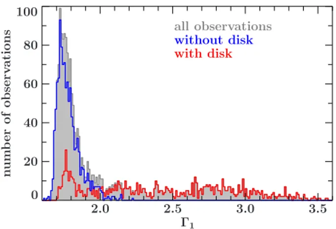
with disk without disk all observations 3.5 3.0 2.5 2.0 100 80 60 40 20 0 Γ1 nu m b er of ob se rv at io ns
Fig. 2. Number of orbit-wise RXTE observations of Cyg X-1 in the B_2ms_8B_0_35_Q mode with a givenΓ1. Shown are both observations
that require a disk (red) and do not require a disk (blue), and the total number of observations (gray).
whenΓ1-values of the models with a disk are used. When
model-ing these seven observations without a disk, all have pronounced residuals at ∼5 keV due to the Xe L-edge (Wilms et al. 2006), no signature of a strong disk in the residuals, and an acceptable reduced χ2 < 1.3. This behavior indicates that the strong disk component and the steeper soft photon index compensate for the instrumental Xe L-edge and are not an adequate description of the source spectrum. We therefore accept the model without a disk as the best fit model for these observations2. TheΓ1-values
for these observations shift from the 2.0–2.2 to the 1.8–2.0 range. We emphasize that if the disk were real and not compensating for sharp calibration features, the removal of the disk compo-nent would result in an increase ofΓ1, contrary to what is seen
here.
We consider the 1980 spectra for which data in the B_2ms_8B_0_35_Q mode is available (see Sect. 2.3). Our fits yield χ2red< 2.5 for all observations, and a fit with χ2red< 1.2 can be achieved for 1721 out of these 1980. In the following, we will useΓ1as a proxy for the spectral state, since all other spectral
parameters show strong correlations withΓ1(Wilms et al. 2006).
In particular, inGrinberg et al.(2013) we have defined the hard state asΓ1 < 2.0, the intermediate state as 2.0 < Γ1 < 2.5, and
the soft state asΓ1 > 2.5. Figure2shows the number of
obser-vations at a givenΓ1; we note not only the good coverage of the
soft and intermediate states, but also the very high number of observations in the hard state.
2.3. Calculation of X-ray timing quantities
We extracted light curves that are strictly simultaneous with the spectral data. For a consistent treatment of the timing proper-ties, we only used observations in the B_2ms_8B_0_35_Q mode, i.e., binned data with eight bands (channels 0–10, 11–13, 14–16, 17–19, 20–22, 23–26, 27–30, and 31–35) and with an intrinsic time resolution of 2−9s ≈ 2 ms, resulting in 1980 RXTE orbits. Because this data mode does not include PCU information, light curves can only be extracted from all PCU units that were op-erating during a particular observation together. Since dead time effects depend on the number of active detectors, we treat each combination of PCUs separately. This approach results in an
2 In our previous study (Grinberg et al. 2013), these seven observations
did not receive any special treatment. This does not, however, influence any of our earlier conclusions.
increase in the number of light curves to 2015, some of them as-sociated with the same spectrum. All analyses in this paper were performed with ISIS 1.6.2 (Houck & Denicola 2000; Houck 2002;Noble & Nowak 2008).
In Table1, we list the channel and energy ranges for the four energy bands that were used throughout this work for calculat-ing the timcalculat-ing properties (bands 3 and 4 combine three channel bands each in order to obtain higher count rates). Most of our data fall into epochs 4 and 5 (Fig.1). The energy range covered by the bands is slightly time dependent because of changes in the high voltage of the PCA, but such small changes will not influence the qualitative analysis presented in this work:
– Band 1 (2.1–4.5 keV) covers the range with a significant contribution from the accretion disk, which can dominate this band in the soft states. At the high soft count rates of the soft states, this band can suffer from telemetry overflow (Gleissner et al. 2004b;Gierli´nski et al. 2008), resulting in artifacts at high frequencies above ∼30–50 keV as can be seen, e.g., in Fig.A.2forΓ1∼ 2.61 and ∼2.713.
– Band 2 (4.5–5.7 keV) covers the soft part of the spectrum above the main contribution of the disk. The band is below the prominent Fe Kα-line at ∼6.4 keV, but since the line is broad its contribution may be significant (Wilms et al. 2006;
Shaposhnikov & Titarchuk 2006;Duro et al. 2011).
– Band 3 (5.7–9.4 keV) includes the Fe Kα-line and covers the spectrum up to the spectral break at ∼10 keV.
– Band 4 (9.4–15 keV) mainly covers the spectrum above the spectral break at ∼10 keV and below the high-energy cut-off. We calculated all timing properties (power spectra [power spec-tral densities, PSD], cross power spectra, coherence, and time lags) following Nowak et al. (1999a) and Pottschmidt et al.
(2003). For the timing analysis, each light curve was split into segments of nbins= 4096 bins, i.e., 8 s length. Timing properties
were calculated for each segment and then averaged over all seg-ments of a given light curve using the appropriate statistics. The mean number of segments used was ∼225, and the mean light curve length therefore ∼30 min. Before rebinning, the values of all timing properties were calculated for discrete Fourier fre-quencies filinearly spaced every∆ f = 1/(nbins∆t) = 0.125 Hz.
The Nyquist frequency of the data is fmax = 1/(2∆t) = 256 Hz,
and the lowest frequency accessible is fmin = 1/(nbins∆t) =
0.125 Hz; i.e., we cover slightly over three decades in temporal frequency. As shown byNowak et al.(1999a), for a source such as Cyg X-1 and using the approach described above, the dead-time-corrected, noise-subtracted PSDs are reliable to at least 100 Hz. The systematic uncertainties for the coherence function are negligible below 30 Hz, and the phase and time lags are de-tectable in the 0.1–30 Hz range (Nowak et al. 1999a, but see also Sect.4.1).
Longer individual segments would enable us to probe lower Fourier frequencies. The lower number of averaged segments per observation would mean higher uncertainties, but generally still reliable results in the case of PSDs. Coherence function and lags are, however, higher order derivative statistics and therefore more sensitive to uncertainties. Thus, to constrain them well, a larger number of segments is necessary; i.e., the individual segments have to be shorter.
3 Telemetry overflow is only a problem for the observations with the
highest count rate, i.e., the observations at the intermediate to soft state transition (Grinberg et al. 2013). Not all observations at a givenΓ1are,
however, affected since spectra with the same Γ1 can vary by a
fac-tor of ∼4. For example for 2.5 < Γ1 < 2.7, the absorbed flux in the
Table 1. Energy bands used for different RXTE calibration epochs.
Epoch Band 1 Band 2 Band 3 Band 4
energy [keV] (channels) energy [keV] (channels) energy [keV] (channels) energy [keV] (channels)
3 ∼1.9b–4.1 (0–10) ∼4.1–5.1 (11–13) ∼5.1–8.3 (14–22) ∼8.3–13.0 (23–35)
4 ∼2.1b–4.6 (0–10) ∼4.6–5.9 (11–13) ∼5.9–9.7 (14–22) ∼9.7–15.2 (23–35)
5a(PCU 0) ∼2.0b–4.6 (0–10) ∼4.6–5.8 (11–13) ∼5.8–9.7 (14–22) ∼9.7–15.4 (23–35)
5a(PCU 1,2,3,4) ∼2.1b–4.5 (0–10) ∼4.5–5.7 (11–13) ∼5.7–9.4 (14–22) ∼9.4–14.8 (23–35)
Notes. Values fromhttp://heasarc.nasa.gov/docs/xte/e-c_table.html. Starting times of epochs are shown in Fig.1. Since the majority of the data is from epoch 5, we cite the band energies throughout this paper as 2.1–4.5 keV for band 1, 4.5–5.7 keV for band 2, 5.7–9.4 keV for band 3, and 9.4–15 keV for band 4.(a)Epoch 5 is defined by loss of the propane layer in PCU 0 due to a micrometeorite impact.(b)Nominally the
0th channel extends to ∼0 keV, but the effective area is negligible below 2 keV (Jahoda et al. 2006).
For PSDs, we choose the normalization of Belloni & Hasinger (1990) and Miyamoto et al. (1991), where the PSD is given in units of the squared fractional rms variability per frequency interval. Since the variance that each frequency con-tributes is given in units of average signal count rate, this nor-malization is most suitable for comparing PSD shapes indepen-dently of source brightness (Pottschmidt 2002). To illustrate the contribution of the variability at a given Fourier frequency, fi, to
the total variability, we show the PSDs in units of PSD times fre-quency, PSD( fi) × fi(Belloni et al. 1997;Nowak et al. 1999a).
We calculated the fractional rms by summing up the contri-butions at individual frequency ranges without employing any modeling of the PSD shape; all rms values in this work are given for the 0.125–256 Hz range.
While the PSD describe the variability of one light curve, the relationship between two simultaneous light curves can be char-acterized by the cross spectral density. Such a cross spectrum is calculated as a product of the Fourier transform of one light curve with the complex conjugate of the Fourier transform of the other light curve.
The coherence function, γ2( fi), a derivative of the norm of
the cross spectrum, measures the Fourier-frequency dependent degree of linear correlation between two time series, in this case the light curves (Vaughan & Nowak 1997). An intuitive geomet-rical interpretation of γ2( f
i) as a length of a vector sum in the
complex plane can be found inNowak et al.(1999a).
For two correlated time series, we can define the Fourier-frequency dependent phase lag φi at a frequency fi as
the difference between the phases of the Fourier transforms of the light curves in both energy bands, calculated as the argu-ment of the complex cross spectrum. The time lag at the fre-quency fi is then given by δt( fi) = φi/(2π fi). Our sign
con-vention is such that the hard light curve lags behind the soft for a positive lag. Since the phase lag, φ, is defined on the in-terval [−π, π[, there is an upper limit for absolute value of the time lag. Experience shows that the lags are below this limit in the considered frequency range in objects such as Cyg X-1 (e.g.,
Nowak et al. 1999a;Pottschmidt et al. 2000,2003;Böck et al. 2011), Swift J1753.5−0127 (Cassatella et al. 2012a), or XTE J1752−223 (Muñoz-Darias et al. 2010).
3. Rms and power spectra
3.1. Evolution of fractional rms with spectral shape
We start with the most basic quantity, the rms variability of the source. As we have previously shown (Grinberg et al. 2013), the total fractional rms in the 0.125–256 Hz frequency band strongly
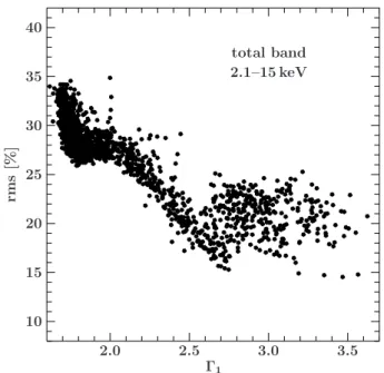
2.1–15 keV total band 3.5 3.0 2.5 2.0 40 35 30 25 20 15 10 Γ1 rm s [% ]
Fig. 3.Fractional rms in the 2.1–15 keV band vs. soft photon indexΓ1.
depends on the spectral state and on the energy band. Here, we analyze this behavior in more detail.
3.1.1. Energy-independent vs. energy-dependent evolution of rms
Figure3 shows how the fractional rms in the 2.1–15 keV band depends on the spectral shape. Here and in the following sec-tions, the errors of the rms are expected to be smaller than the spread of the shown correlations at any giveΓ1. The rms reaches
its highest values of ∼34% at the lowestΓ1of ∼1.6. TheΓ1-rms
correlation is negative belowΓ1 ≈ 1.8, then flat untilΓ1 ≈ 2.0,
again negative untilΓ1 ≈ 2.5–2.7, and finally flattens out at an
rms of ∼20% but with a larger scatter.
The energy-dependent fractional rms reveals where most of this variability in the total 2.1–15 keV band comes from in the different spectral states. Figure1 shows the temporal evolution of the fractional rms in the soft band 1 and the hard band 4 (2.1– 4.5 keV and 9.4–15 keV) over the lifetime of RXTE. During hard states, the variability is high at about ∼30% in both bands. In the soft state, the rms drops to 10–20% in band 1, but in band 4 it is slightly larger than in the hard state. The intermediate state is associated with a decrease in rms in both bands. This behavior is better visualized in Fig.4, where we plot rms as a function ofΓ1
2.1–4.5 keVband 1 3.5 3.0 2.5 2.0 40 35 30 25 20 15 10 4.5–5.7 keV band 2 3.5 3.0 2.5 2.0 5.7–9.4 keVband 3 3.5 3.0 2.5 2.0 9.4–15 keVband 4 3.5 3.0 2.5 2.0 Γ1 rm s [% ] Γ1 Γ1 Γ1
Fig. 4.Fractional rms in the 0.125–256 Hz frequency band for different energy bands vs. the soft photon index, Γ1, of the broken power law fits.
Table 2. Spearmann ρ correlation coefficients for Γ1–rms correlation.
Band ρΓ1<1.8 ρ1.8 <Γ1<2.0 ρ2.0 <Γ1< 2.65 ρ2.65 <Γ1 total −0.61 0.21b −0.89 0.02c 1 −0.50 0.25 −0.89 −0.28 2 −0.55 0.19 −0.88 0.43 3 −0.62 −0.064a −0.84 0.65 4 −0.64 −0.31 −0.70 0.68
Notes. All null hypothesis probabilities P < 10−4except for (a) with
P= 0.18 ;(b)with P= 0.21 ; and(c)with P= 0.66.
behavior (see Table2for correlation coefficients for bands 1–4
and the total band).
– Γ1 < 1.8: the Γ1–rms correlation is negative and becomes
stronger at higher energies in the individual and the total bands;
– 1.8 ≤Γ1 < 2.0: the correlation is positive for bands 1 and 2
and negative for band 4. In band 3, the rms values are con-sistent with being uncorrelated withΓ1, an understandable
behavior given the change of sign in adjacent bands. In the total band, there is no correlation;
– 2.0 ≤Γ1 < 2.65: the correlation is strong and negative in all
bands including the total, though it becomes less steep with increasing energy;
– 2.65 ≤ Γ1: the correlation changes from negative in band 1
(note the negative ρ-value in Table2) to positive in bands 2–4 and becomes stronger with increasing energy. The total rms in the 2.1–15 keV band shows no correlation with spec-tral shape. There is a slight indication of further structure atΓ1∼ 2.8–2.9 in energy bands 2–4.
The changes in slope of the rms-Γ1relationship atΓ1 ∼ 1.8 and
Γ1∼ 2 are present both when considering only observations that
do not require a disk and only observations that do require a disk. These changes are therefore not artifacts caused by the choice of spectral model used to measureΓ1. ForΓ1 > 2, the number of
observations that do not require a disk is negligible (Fig.2). We also note that the Γ1 thresholds represent approximate values,
since the transition from one behavior pattern to the other is not clearly defined.
A compact representation of the rms behavior is given by the ratio of the rms values between the different bands (Fig.5). The relation is tight enough that it can serve as a simple check for the spectral shape of the source without any model assumptions. We used it, for example, to check our broken power law fits for out-liers as described above in Sect.2.2. We emphasize that because of the strong energy dependence of the rms, the total fractional rms in the 2.1–15 keV band (Fig.3) cannot be used to determine whether one soft state observation is softer than another in terms
9.4–15 keV/4.5–5.7 keV rms4/rms2: 9.4–15 keV/2.1–4.5 keV rms4/rms1: 3.5 3.0 2.5 2.0 2.5 2.0 1.5 1.0 Γ1 rm s ra ti o
Fig. 5.Ratio of fractional rms in different energy bands (band 1 – rms1,
band 2 – rms2, band 4 – rms4,) vs. soft photon indexΓ1.
of relative Γ1, while the rms at energies above ∼6 keV or the
ratio of rms at different energies (Fig.5) can.
The energy-independent analyses of RXTE data by
Pottschmidt et al.(2003), who use the 2.1–15 keV range, and
Axelsson et al.(2006), who use the 2–9 keV range, are consistent with the rms evolution presented here, although different time ranges are covered. A decrease in the rms as the source softens was also observed at higher energies, namely in the 10–200 keV range using Suzaku-PIN and Suzaku-GSO byTorii et al.(2011) and in the 27–49 keV band using INTEGRAL-SPI byCabanac et al.(2011), although neither of them observed a full soft state withΓ1 & 2.5, where our analysis shows an increase in the rms
above ∼6 keV.
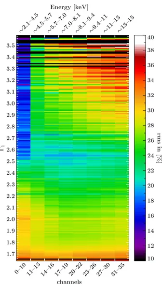
To better understand the behavior of rms with both energy and spectral shape, we looked at the behavior of these quanti-ties in the eight bands of the B_2ms_8B_0_35_Q mode (Fig.6). For each energy band, we determined the average fractional rms from all observations during which a similar photon spectral shape was found. Two photon spectra are considered to be sim-ilar if their respectiveΓ1values fall into the same bin of a
lin-ear grid with steps of∆Γ1 = 0.01 between Γ1,min = 1.64 and
Γ1,max = 3.59. The trends shown in Fig.4and Table2are
con-firmed. The higher energy resolution allows us to see the grad-ual increase in fractional rms withΓ1for Γ1 & 2.7 at all
ener-gies above 4.5 keV. The increase steepens at higher enerener-gies. For 1.8 <Γ1 < 2.3, the variability is lower above 4.5 keV than below
Energy [keV] ∼13– 15 ∼11– 13 ∼9.4– 11 ∼8.1– 9.4 ∼7.0– 8.1 ∼5.7– 7.0 ∼4.5– 5.7 ∼2.1– 4.5 channels 31 –35 27–3 0 23–2 6 20–2 2 17–1 9 14–1 6 11–1 3 0–10 3.5 3.4 3.3 3.2 3.1 3.0 2.9 2.8 2.7 2.6 2.5 2.4 2.3 2.2 2.1 2.0 1.9 1.8 1.7 40 38 36 34 32 30 28 26 24 22 20 18 16 14 12 10 Γ1 rm s in [% ]
Fig. 6.Evolution of fractional rms between 0.125–256 Hz in the eight binned channels of the B_2ms_8B_0_35_Q mode with the X-ray spec-tral shape represented by the soft photon index Γ1. Black horizontal
lines are photon indices for which no data are available.
that energy, but the decrease in rms with energy does not appear smooth and shows an indication of recovery above 11 keV.
Examples of rms spectra shown byGierli´nski et al.(2010) agree with Fig.6, but these authors do not observe an increase in the rms above 11 keV for 1.8 <Γ1 < 2.3. Such an increase is
present (but not pointed out) in the one Cyg X-1 rms spectrum shown byMuñoz-Darias et al.(2010). In the 10–200 keV range,
Torii et al.(2011) show that the fractional rms spectra remain largely flat in hard and intermediate4 states and that the
inter-mediate state shows less variability than the hard state; i.e., the behavior presented here for the 2.1–15 keV range continues at higher energies.
3.2. Evolution of PSDs with spectral shape
Having discussed the overall source variability by studying the rms, we now turn to the Fourier frequency-dependent variabil-ity. For our analysis of the change of PSD shapes with spec-tral state, we choose an approach that does not require us to
4 Torii et al.(2011) speak only of hard states with high ASM count
rates; a comparison with ASM-HID-based state definition ofGrinberg et al.(2013) shows that these states are intermediate.
Γ2.612.72.82.93.03.13.23.33.43.5 2.5 2.4 2.3 2.2 2.1 2.0 1.9 1.8 1.7 100 10 1 2.4 2.2 2.0 1.8 1.6 1.4 1.2 1.0 0.8 0.6 0.4 0.2 Fo ur ie r fr eq ue nc y f [H z] 2. 1– 15 ke V PSD ×f [rms2× 102]
Fig. 7.Evolution of PSDs in 2.1–15 keV band (sum of bands 1–4 and full energy range of the B_2ms_8B_0_35_Q mode) with spectral shape. The color scale represents averaged PSD( fi) × fi values at individual
Fourier frequencies fi. In this and in all following figures, black vertical
lines are photon indices for which no data are available.
model the PSDs and thus does not introduce any assumptions on identification of possible components in individual PSDs and their evolution. For possible pitfalls of such assumptions, see Sect.5.2.
We visualize the evolution of the PSD components as a color map in fi–Γ1-space following an idea ofBöck et al.(2011). As
in the analysis of the rms behavior, we define a grid with steps of∆Γ1 = 0.01 between Γ1,min= 1.64 and Γ1,max = 3.59 and 100
equally spaced steps in logarithmic frequency between 0.125 Hz and 256 Hz. When mapping linear Fourier frequencies to this logarithmic grid, some bins remain empty. We allocate these to adjacent bins containing at least one Fourier frequency, equally divided between higher and lower bins. In the following, we first discuss the energy-independent behavior of the power spectra in Sect.3.2.1, and then turn to the energy-dependent variability in Sect.3.2.2.
3.2.1. Energy-independent evolution of PSDs with spectral shape
Most previous works address the timing quantities in an energy-independent way. Because of the strong changes in spectral shape (seeNowak et al. 2012, for examples of broadband spec-tra of Cyg X-1 in hard and soft states) and hence count rate ratios at different energies, extrapolation from energy-band dependent quantities to the full energy range across all spectral states is nontrivial. Thus, we first address the full 2.1–15 keV range and show the evolution of these PSDs with spectral shape in Fig.7.
For 1.75 < Γ . 2.7, two strong variability components are present. Previous work has shown that such components can be modeled well as (often zero-centered) Lorentzians (e.g.,Nowak 2000), and by visual comparison we can identify the components with the two Lorentzians ofBöck et al.(2011) and with the two lowest frequency Lorentzian components ofPottschmidt et al.
(2003). In the spirit of the approach chosen here that avoids de-pending on models for the variability, we label the lower fre-quency variability component as component 1 and the higher frequency variability component as component 2. Both compo-nents shift to higher frequencies asΓ1softens (see alsoCui et al.
1997;Gilfanov et al. 1999; Pottschmidt et al. 2003;Axelsson et al. 2005;Shaposhnikov & Titarchuk 2006;Böck et al. 2011). The two components appear to have roughly similar strengths. In the PSDs shown in the 2.1–15 keV band, we observe that com-ponent 2 disappears atΓ1 ≈ 2.5, so that the PSD is dominated
by component 1 for 2.5 < Γ1 < 2.7. We also draw attention to
the low variability at the lowest frequencies in theΓ1 ∼ 2.3–2.6
range. At the highest frequencies, the PSDs in allΓ1-ranges are
dominated by low statistics and therefore noise.
For Γ1 . 1.75, we see additional power at frequencies
above ∼2 Hz, i.e., above the frequencies assumed by compo-nents 1 and 2 in this Γ1-range. This behavior is consistent
with the appearance of the third Lorentzian component in the very hard observations analyzed by Pottschmidt et al.(2003) and Axelsson et al.(2005). We note that the hardest obser-vations analyzed by these authors are from before 1998 April, i.e., during a time not covered by the data mode we use, while the hardest spectra analyzed here were ob-served during the long hard state between 2006 and mid-2010 (Nowak et al. 2011;Grinberg et al. 2013). Interestingly, the overall variability amplitude increases in thisΓ1-range at all
frequencies below ∼10 Hz.
ForΓ1& 2.7, the variability is generally low, consistent with
low total rms in this range (Fig. 3). It is continuous, without pronounced components, and strongest at the lowest frequencies and decreases towards higher frequencies.
3.2.2. Energy-dependent evolution of PSDs with spectral shape
The energy-dependent evolution of the fractional rms (Sect.3.1) hints at the PSDs being highly dependent on the energy band considered, especially in the soft spectral state. The shape of the PSDs in all four energy bands is shown in Fig. 8. These maps emphasize the dominant components and use a linear color scale for the PSD( fi) × fivalues, while usually individual
power spectra are presented on a logarithmic PSD( fi) × fi-axis
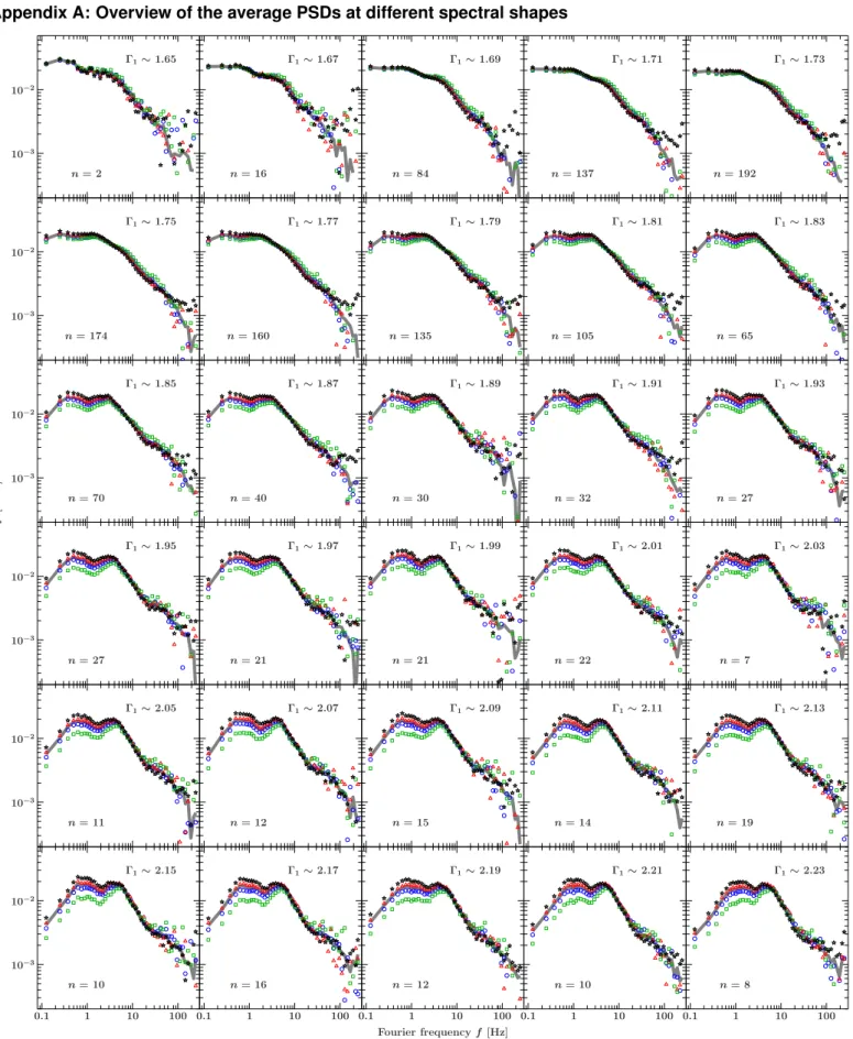
(Figs.A.1−A.4).
For 1.75 . Γ1 . 2.7, we observe the same two
variabil-ity components as in the energy-independent PSDs. Both com-ponents become weaker with increasing energy. The amplitude of component 1 decreases faster than the amplitude of compo-nent 2: compocompo-nent 1 is stronger than compocompo-nent 2 in band 1 (4.5–5.7 keV), but in band 4 (9.4–15 keV) component 2 is more pronounced. Especially in theΓ1≈ 2.4–2.6 range, component 1
dominates the lower energy bands, but component 2 the higher energy bands.
For Γ1 . 1.75, the shape of the PSDs appears
energy-independent, as opposed to the softer observations. The addi-tional higher frequency component discussed in Sect. 3.2.1 is present in all bands.
ForΓ1 & 2.7, the variability shows a behavior that is
funda-mentally different from the behavior of the two components in the 1.75. Γ1 . 2.7 range, as already indicated by the different
behavior of the rms in Sect.3.1. In band 1, the overall variabil-ity is low, consistent with the evolution of the total rms. What variability there is seems to show a slight trend towards lower frequencies with increasingΓ1 (see also Fig.A.3). In bands 2
to 4, the variability increases strongly with increasing energy of the band and within an energy band with increasingΓ1.
FiguresA.1–A.4present average PSDs at different spectral shapes to facilitate comparison with previous work. While the continuous change in the PSD is better illustrated in the ap-proach of Fig. 8, two effects are better represented by looking at fi-PSD( fi) × fi-plots of PSDs. First, in the frequency range
considered here, the power spectra at energies above ∼5 keV are similar for the hardest observations withΓ1 < 1.75 and the
softest observations with Γ1 > 3.15, as can be easily seen on
Figs.A.1–A.4and as shown for two exampleΓ1values in Fig.9.
100 10 1 100 10 1 100 10 1 Γ12.72.82.93.03.13.23.33.43.5 2.6 2.5 2.4 2.3 2.2 2.1 2.0 1.9 1.8 1.7 100 10 1 2.4 2.2 2.0 1.8 1.6 1.4 1.2 1.0 0.8 0.6 0.4 0.2 9. 4– 15 ke V (b an d 4) 5. 7– 9. 4 ke V (b an d 3) 4. 5– 5. 7 ke V (b an d 2) 2. 1– 4. 5 ke V (b an d 1) Fo ur ie r fr eq ue nc y f [H z] PSD ×f [rms2× 102]
Fig. 8.Evolution of the PSDs with spectral shape represented by the soft photon indexΓ1of the broken power law fit in four energy bands
(see Table1). The color scale represents averaged PSD( fi) × fivalues at
individual Fourier frequencies fi.
While the different dependence of the PSDs themselves on the energy and the different cross-spectral properties (see Sect.4) suggest a different origin for these power spectra, the shapes can easily be confused, especially when data are of lower qual-ity. Secondly, there are indications of a weak third hump above 10 Hz for 1.75 . Γ1 . 2.15 that is not visible in this range in
Fig.8and that corresponds to the higher frequency Lorentzian component L3 modeled by Pottschmidt et al. (2003). For the
hardest observations withΓ1 . 1.75, there are also hints of a
further component at ∼30 keV (see alsoRevnivtsev et al. 2000;
Nowak 2000;Pottschmidt et al. 2003).
An energy-dependent approach to both rms and PSDs is clearly necessary for understanding the variability components in different states because they show strikingly different behavior with the changing energy, which is otherwise missed. This result may be especially important when comparing black hole binaries to AGN and cataclysmic variables, where at the same energy we probe different parts of the emission (see also Sect.5.3).
Γ1∼ 3.49 Γ1∼ 1.67 5.7–9.4 keV 100 10 1 0.1 10−2 10−3 Γ1∼ 3.49 Γ1∼ 1.67 2.1–15 keV 100 10 1 0.1 P SD × f [r m s 2] Fourier frequency f [Hz]
Fig. 9. Comparison of average PSDs for Γ1 ∼ 1.67 (blue stars) and
Γ1 ∼ 3.49 (red squares). PSDs are calculated for a logarithmically
binned grid with d f / f = 0.15. Each PSD is the average of all n PSDs falling within theΓ1 ± 0.01 interval for the givenΓ1values. Left : band
2 (5.7–9.4 keV). Right : total band (2.1–15 keV).
3.2.3. Discussion of PSD shapes
The frequency shift of the variability components of the PSDs in the RXTE range with the softening of the source in the hard and intermediate states continues at higher energies (Cui et al. 1997;
Pottschmidt et al. 2006; Cabanac et al. 2011) up to ∼200 keV (Torii et al. 2011), even though such high energy analyses are rare. The different energy dependence of the components has been previously noted for individual observations, both for the presented energy range and above (Cui et al. 1997;Nowak et al. 1999a; Pottschmidt et al. 2006; Böck et al. 2011), but never shown for such a comprehensive data set as presented in this work.
The ∼ f−1-variability of the soft state PSDs can be described by a power law, while the power spectra of intermediate states are often modeled with a combination of Lorentzian components with (cut-off) power law (e.g.,Cui et al. 1997;Axelsson et al. 2005, 2006).Cui et al. (1997) have noted that the power law component becomes stronger with increasing energy for individ-ual soft state observations up to 60 keV; we observe this effect, which has also been noted byChurazov et al.(2001), up to our maximum energy of 15 keV. We also clearly see that at ener-gies above 4.5 keV the variability grows with increasingΓ1for
Γ1> 2.7, but decreases below 4.5 keV.
Our approach does not allow us to track the weak power law in the intermediate state, especially given that our lowest acces-sible frequency is 0.125 Hz. However, we see that the power law dominates the PSDs forΓ1 & 2.7 – the abrupt change can also
be seen in the cross spectral quantities presented in the next sec-tion (Sect.4). In particular, forΓ1 & 2.7, the coherence, which
shows a dip for 2.5 < Γ1 < 2.7, recovers (Sect.4.1); the time
lag spectra lack the previously present structure (Sect.4.2); and the averaged time lags show an abrupt drop and no correlation withΓ1 forΓ1 & 2.65 (Sect.4.3). Cross-spectral quantities are
thus clearly crucial for gaining a better understanding of the vari-ability of the source and are discussed in the following section.
4. Coherence and time lags
4.1. Evolution of Fourier-dependent coherence with spectral shape
We calculate maps of the coherence function, γ2
h,s( fi) where
h ∈ {4, 3, 2} is the harder band and s ∈ {3, 2, 1} is the respective softer band, using the same grid as in our analysis of the power spectra (Sect. 3.2). Figure 10 shows maps of the coherence
100 10 1 100 10 1 Γ1 3.5 3.4 3.3 3.2 3.1 3.0 2.9 2.8 2.7 2.6 2.5 2.4 2.3 2.2 2.1 2.0 1.9 1.8 1.7 100 10 1 coherence function γ2 1.0 8 1.06 1.04 1.02 1.00 0.98 0.96 0.94 0.92 0.90 0.88 0.86 9. 4– 15 to 5. 7– 9. 4 ke V 9. 4– 15 to 4. 5– 5. 7 ke V 9. 4– 15 to 2. 1– 4. 5 ke V Fo ur ie r fr eq ue nc y f [H z]
Fig. 10. Evolution of the coherence, γ2, with spectral shape
repre-sented by the soft photon indexΓ1of the broken power law. The color
scale represents averaged γ2values at individual Fourier frequencies f i.
Upper panel: γ2
4,3between bands 4 and 3, middle panel: γ 2
4,2between
bands 4 and 2, lower panel: γ2
4,1between bands 4 and 1.
function between band 4 and bands 1–3. By eye, we can identify an envelope in all shown coherence functions that follows the high frequency outline of the dominant variability components of the power spectra (Sect.3.2). Outside of this envelope, the coherence fluctuates strongly.
To assess whether the envelope is an intrinsic feature of the source or whether it is due to the low signal at the high frequen-cies, we simulate example light curves with typical spectra and PSDs for different values of Γ1. To do so, we use Monte Carlo
simulation with the software package SIXTE (SImulation of X-ray TElescopes) developed for the analysis of various X-ray instruments (Schmid 2012). For each selected PSD provided in the SIMulation inPUT (SIMPUT) file format5, the simulation software obtains a light curve using the algorithm ofTimmer & König(1995). Here, we use the PSDs in the full 2.1–15 keV band as input PSDs. Based on this light curve, a sample of X-ray photons is generated with the Poisson arrival process genera-tor ofKlein & Roberts(1984). The energies of the photons are distributed according to the observed spectrum, which is cho-sen as constant throughout the simulation. The photons are then processed through a model of the PCA taking instrumental ef-fects into account, such as energy resolution and dead time. The
5 http://hea-www.harvard.edu/HEASARC/formats/
output of this model is a list of simulated events as detected with the PCA, which is converted back to light curves in chosen chan-nel or energy bands for the subsequent analysis. As the spectral shape remains unchanged and only the rate of generated pho-tons, i.e., the normalization of the spectrum, varies with the light curve, the variability in different energy bands is, by definition, coherent.
We simulate light curves in bands 4 and 1 and calcu-late γ2
4,1( fi) as for observed light curves. The trends we observe
in γ24,1( fi) are the same as for observed light curves: the
coher-ence function is ∼1 below approximately 10 Hz and then shows strong variations above that frequency. This threshold frequency weakly depends on state and decreases towards lower frequen-cies in the soft state. We therefore conclude that the envelope seen in the coherence function plots is not source-intrinsic but a consequence of the low signal at higher frequencies.
A feature not present in our simulations of ideally coherent light curves is the decrease in coherence for 2.35. Γ1 . 2.65 in
a region that seems to follow the shape of the PSD components 1 and 2 (see Sect.3.2.1). This decrease is most evident in γ2
4,1( fi),
where the coherence values drop below 0.85, but is also visible in γ24,2( fi) and indicated in γ24,3( fi) (Fig.10).
ForΓ1 & 2.65, the coherence recovers, although the values
between the 9.4–15 keV and 2.5–4.5 keV bands remain signif-icantly lower (∼0.92–0.94) than between 9.4–15 keV and the 4.5–5.7 keV and 5.7–9.4 keV bands. The coherence seems also noisier, although this is likely due to the lower number of observations in the soft state.
4.2. Evolution of Fourier-dependent time lags with spectral shape
The time lags show a strong power law dependence on the Fourier frequency with δt( fi) ∝ fi−0.7 (Nowak et al. 1999a,
and references therein), so that we consider the fraction δt( fi)/ fi−0.7 B ∆δt to visualize structures in the time lag spec-tra and again follow the approach from Sect.3.2. In Fig.11, we present maps of∆δt for band combinations showing the largest lags, i.e., bands with largest separation in energy (Miyamoto et al. 1988;Nowak et al. 1999a). In the phase lag representa-tion, the largest lags between the 2.1–4.5 keV and 9.4–15 keV bands do not exceed ∼0.5 rad, so that the time lags are well de-fined, and the features in Fig.11are not due to the phase lag to time lag conversion (see Sect.2.3).
If the lags strictly followed δt( fi) ∝ fi−0.7, then the only
struc-ture∆δt would show would be a gradient with changing Γ1,
cor-responding to the known changes in average lag with state (e.g.,
Pottschmidt et al. 2003). Such a gradient is indeed visible, with the lags obtaining highest values atΓ1∼ 2.5–2.6.
ForΓ1. 2.7, however, there is a fi-dependent structure
over-laid on theΓ1-dependent gradient. This structure seems to track
the two components 1 and 2 of the PSDs (see Sect.3.2) and is visible for all energy band combinations. A correlation between the features of the PSDs and of time lag spectra has been sug-gested in Cyg X-1 byNowak(2000), but to our knowledge has not been shown for a wide range of spectral states and therefore PSD shapes for any black hole binary previously.
ForΓ1 & 2.7, the lag spectrum shows no structure and has
lower values than for harderΓ1. No evolution withΓ1 is seen in
the soft state.
ForΓ1 < 1.75, where the PSDs show increased variability
and a possible additional component at higher frequencies, no corresponding changes can be seen in the ∆δt maps. The two
Γ1 3.23.33.43.5 3.1 3.0 2.9 2.8 2.7 2.6 2.5 2.4 2.3 2.2 2.1 2.0 1.9 1.8 1.7 100 10 1 30 25 20 15 10 5 0 Γ12.72.82.93.03.13.23.33.43.5 2.6 2.5 2.4 2.3 2.2 2.1 2.0 1.9 1.8 1.7 100 10 1 25 20 15 10 5 0 Γ1 3.23.33.43.5 3.1 3.0 2.9 2.8 2.7 2.6 2.5 2.4 2.3 2.2 2.1 2.0 1.9 1.8 1.7 100 10 1 20 18 16 14 12 10 8 6 4 2 0 -2 Fo ur ie r fr eq ue nc y f [H z] 9. 4– 15 to 2. 1– 4. 5 ke V timelag / f−0.7[ms/Hz−0.7] Fo ur ie r fr eq ue nc y f [H z] 9. 4– 15 to 4. 5– 5. 7 ke V timelag / f−0.7[ms/Hz−0.7] Fo ur ie r fr eq ue nc y f [H z] 5. 6– 9. 4 to 2. 1– 4. 5 ke V timelag / f−0.7[ms/Hz−0.7]
Fig. 11.Evolution of time lags δt in the δt( fi)/ fi−0.7 B ∆δt
represen-tation with spectral shape represented by the soft photon indexΓ1 of
the broken power law. The color scale (note the different scales for the bands presented) represents averaged∆δt values at individual Fourier frequencies fi. Positive lags mean that the hard photons lag behind the
soft.
components 1 and 2 of the hard and intermediate state PSDs are, however, clearly visible in the time lag maps.
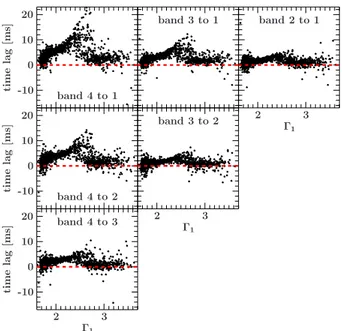
4.3. Evolution of average time lag with spectral shape The usual measure for time lags in the literature are averaged lags δtavg in the 3.2–10 Hz band (e.g.,Pottschmidt et al. 2003;
Böck et al. 2011). To facilitate comparisons, we follow the ap-proach of the previous work: we rebin each raw time lag spec-trum to a logarithmically spaced frequency grid with d f / f = 0.15 and then calculate an average value for the 3.2–10 Hz band. The average time lags (Fig. 12) are larger for bands with a greater difference in energy, but all combinations of energy bands show the same nonlinear trends withΓ1: a strong increase
Table 3. Spearman correlations coefficients ρ and null hypothesis probabilities P for the correlation of averaged time lags in the 3.2–10 Hz band withΓ1for different Γ1ranges (see also Fig.12).
Band 4 to 1 Band 4 to 2 Band 4 to 3 Band 3 to 1 Band 3 to 2 Band 2 to 1
ρ P ρ P ρ P ρ P ρ P ρ P
Γ1< 2.65 0.79 0a 0.72 0a 0.65 0a 0.3 0a 0.52 0a 0.52 0a
Γ1≥ 2.65 −0.14 0.01 −0.12 0.03 −0.06 0.30 −0.09 0.10 −0.10 0.06 −0.09 0.11
Notes.(a)Within numerical accuracy.
band 4 to 1 20 10 0 -10 band 4 to 2 20 10 0 -10 band 4 to 3 3 2 20 10 0 -10 band 3 to 1 band 3 to 2 3 2 band 2 to 1 3 2 ti m e la g [m s] ti m e la g [m s] Γ1 ti m e la g [m s] Γ1 Γ1
Fig. 12.Averaged time lag in the 3.2–10 Hz range vs. soft photon index of the broken power law fitsΓ1 for all combinations of energy bands
(band 1: 2.1–4.5 keV, band 2: 4.5–5.7 keV, band 3: 5.7–9.4 keV, band 4: 9.4–15 keV). Zero time lag is represented by the dashed red line.
drop atΓ1 ∼ 2.65 that has also been noted by, e.g.,Pottschmidt
et al.(2000) andBöck et al.(2011).
Spearman rank coefficients between the average time lag, δtavg, and the soft photon index,Γ1, forΓ1< 2.65 and Γ1≥ 2.65
are listed in Table 3. In all bands, δtavg is strongly positively
correlated with Γ1 for Γ1 < 2.65 and not correlated or weakly
negatively correlated with Γ1 for Γ1 ≥ 2.65. The weak
neg-ative correlation may be an artifact of the choice of threshold Γ1-values of 2.65. Spearman rank coefficients and their low null
hypothesis probabilities do, however, not imply a linear corre-lation: the relationship forΓ1 < 2.65 appears nonlinear, with a
bend atΓ1∼ 1.8–1.9 and a stronger than linear increase towards
higherΓ1(Fig.12, especially time lag between bands 4 and 1).
4.4. Comparison with previous results for coherence and lags
Cross-spectral analysis is generally less present in the litera-ture, and an analysis of the Fourier-dependent coherence func-tion and time lags for Cyg X-1 across the full range of spec-tral states of the source is undertaken in this paper for the first time. However, the available previous results agree well with the long-term evolution presented here, in particular for coherence in different spectral states (Cui et al. 1997; Pottschmidt et al. 2003; Böck et al. 2011) and for average time lags in hard and intermediate states (Pottschmidt et al. 2003;Böck et al. 2011). The return to low values in the soft state has been noted before
(Pottschmidt et al. 2000;Böck et al. 2011), but the abruptness of the change withΓ1can only be seen for an extensive data set,
such as the one presented here, or for the extremely rare, almost uninterruptedly covered transitions such as the one analyzed by
Böck et al.(2011).
In a different approach, Skipper et al.(2013) compute the cross correlation function between the photon index and the 3–20 keV count rate of Cyg X-1 and find different shapes in dim hard states, bright hard states, and soft states. All their hard state cross correlation functions show asymmetries that can only be explained if a part of the hard count rate lags the soft, consistent with our observations of a hard lag. Their dim hard states corre-spond to the hardest states observed byPottschmidt et al.(2003) in 1998. These hardest states are similar to our data falling into the Γ1 < 1.8 range, i.e., mostly data from the long hard
state 2006 to 2010 (Nowak et al. 2011;Grinberg et al. 2013), and therefore before the first bend of the δtavg–Γ1 correlation
(Sect.4.3). Data taken during these states include further com-ponents in the PSD, which can also be seen in the hardest obser-vations presented here. Similar evidence of growing hard lags as the source transits into the intermediate state was also found by
Torii et al.(2011) in cross correlation function of the 10–60 keV and 60–200 keV Suzaku light curves.
The double-humped structure in the phase lag spectra of Cyg X-1 (Sect.4.2, forΓ1 . 2.7) has been suggested since the
late 1980s (Miyamoto & Kitamoto 1989). Correlated features in the PSDs and time lag spectra were noted for individual observa-tions (Cui et al. 1997;Nowak 2000), but there has been only little work on the systematic evolution of these features with spectral state. We stress the importance of this approach by comparing our results toPottschmidt et al. (2000), who discuss time lag spectra for individual observations in different states and argue on their basis for a similar shape of the time lag spectra in hard and soft states. While the f−0.7-behavior is indeed dominant in both states and individual hard and soft observations therefore appear similar, we see features correlated with PSD components in the hard but not in the soft state (Fig.11).
5. Using the variability of Cyg X-1 as a template for other black holes
Before discussing possible implications of the observed vari-ability patterns on physical interpretations of the varivari-ability in Sect. 6, we first address the importance of our model-independent approach for long-term timing analysis and the im-plications for the interpretation and further analysis of variability components in other sources.
5.1. Cyg X-1 and the canonical picture of states and state transitions
A comprehensive analysis of all sources observed with RXTE is out of the scope of this work. In contrast to most transient black
hole binaries (see, e.g., Klein-Wolt & van der Klis 2008, for a sample study) and most notably the canonical X-ray transient GX 339−4 (Belloni et al. 2005), Cyg X-1 does not show strong narrow quasi periodic oscillations (QPOs)6, although there is
ev-idence of short-lived QPOs (Pottschmidt et al. 2003, Remillard, priv. comm.). Common for black hole binaries, however, seem to be the two flavors of the hard state with different X-ray timing properties (e.g.,Cassatella et al. 2012a, for Swift J1753.5−0127; and Done & Gierli´nski 2005, for XTE J1550−564), the fre-quency shift of the main variability components in the hard and intermediate states (e.g, Klein-Wolt & van der Klis 2008), and the sharp change in timing behavior as the source transits into the soft state (e.g.,Nowak 1995;Klein-Wolt & van der Klis 2008), all shown here in unprecedented detail for Cyg X-1.
In the canonical picture of the black hole binary states, the rms drops to a few percent in the soft state (Belloni 2010). The rms of Cyg X-1 does not assume such low values, even when the 2.1−4.5 keV band is considered (Fig.3). However, Cyg X-1 is not the only source showing such behavior: for example, a complex, energy-dependent rms behavior in the soft state with the rms remaining flat in the 3.2–6.1 keV band and increasing in the 6.1–10.2 keV band has also been observed in the 2010 out-burst of MAXI J1659−152 (Muñoz-Darias et al. 2011), a source that, like Cyg X-1, does not show a purely disk-dominated soft state. Similar to Cyg X-1, MAXI J1659−152 also shows increased time lags in the intermediate state (Muñoz-Darias et al. 2011). Correlated features in power and time lag spec-tra were also seen in, e.g., GX 339−4 (Nowak 2000) and Swift J1753.5−0127 (Cassatella et al. 2012b).
5.2. The identification of the variability components
Assuming that we can use Cyg X-1 as a template for the long-term variability of PSDs and cross-power quantities in other black hole binaries, we can avoid misidentification of PSD com-ponents in the different spectral states. This is often a problem in observations that are less well sampled than desirable and there-fore do not allow tracking the frequency dependency of compo-nents in the PSDs with spectral shape. We note, however, that as a persistent source, Cyg X-1 may not cover some of the extreme behavior of the transient sources.
For example, in their study of a state transition of XTE J1650−500,Kalemci et al.(2003) model the power spec-trum in the intermediate state as a Lorentzian, which shifts to a higher frequency when comparing the power spectra taken from the 3–6 keV and the 6–15 keV data. A comparison with Fig.8
shows that the observations ofKalemci et al.(2003) could be ex-plained if this source falls in the spectral range where the lower energy bands are dominated by component 1 and the higher en-ergy bands by component 2 (2.4. Γ1. 2.7 for Cyg X-1).
A comparison with Figs.7and8also reveals a different in-terpretation of the RXTE observations of Swift J1753.5−0127. Here, Soleri et al. (2013) see two broad peaks that decrease in frequency with increasing spectral hardness, and then jump again to higher frequencies for the hardest observations. The overall pattern seen in our Cyg X-1 data suggests the alterna-tive interpretation that for softer observations the model ofSoleri et al. (2013) tracks components 1 and 2, while for the harder
6 Here and in the rest of this work we use the term “QPO” exclusively
for narrow features and do not use the term to describe the broader humps as done, e.g., by Shaposhnikov & Titarchuk(2006). The dif-ference in terminology is phenomenological and does not necessarily imply an assumption of a different origin for the features.
observations, the model picks up the prominent component 3 that appears at higher frequencies than components 1 and 2 in our hardest observations (see alsoPottschmidt et al. 2003). 5.3. Variability in black hole binaries and AGN
Since the physics of accretion is expected to be similar for com-pact objects of different mass, the characteristic frequencies seen in the power spectra are expected to scale with mass. AGN are therefore expected to show timing behavior similar to black hole binaries, albeit at higher timescales of hours to years (McHardy et al. 2006). Timing analysis of AGN is, however, notoriously complicated because of the low fluxes and the low frequencies, which are hard to sample well.
PSDs of AGN generally suffer from lower signal-to-noise and sparser sampling than those of black hole binaries, and they are usually modeled with either power laws or broken/bending power laws (see, e.g.,González-Martín & Vaughan 2012, for analysis of a large sample observed with XMM-Newton). More complex model shapes with two bends (going to a power-law slope of 0 at the lowest temporal frequencies) or two Lorentzians have only been fit in one case so far, namely Akn 564 (McHardy et al. 2007)7. AGN generally show high coherence that drops at higher frequencies and Fourier frequency- and energy-dependent time lags (Vaughan et al. 2003; Markowitz et al. 2007;Sriram et al. 2009). In Akn 564, the time lag spec-tra show features at frequencies corresponding to changes in the components dominating the PSD (McHardy et al. 2007). On short timescales, AGN show soft lags between energy bands dominated by soft excess and the power law (e.g.,Fabian et al. 2009;De Marco et al. 2013), but we note that the mass-scaled frequency range covered by these observations is not accessible for lag studies in X-ray binaries8. Although they differ in details,
the correlations between spectral and timing parameters in AGN and binaries also seem to follow similar trends (Papadakis et al. 2009) and appear to be at least comparable.
As we have seen above (Sects.3.2.2and5.1), PSD shapes in Cyg X-1 and other black hole binaries are, however, strongly energy-dependent. The energy dependence of AGN PSDs has not been studied as well, but relatively higher energy PSDs tend to show either higher break frequencies (e.g., McHardy et al. 2004;Markowitz et al. 2007) or flatter power-law slopes above the break (Nandra & Papadakis 2001; Vaughan et al. 2003;
Markowitz 2005) with PSD shape flattening and normalization dropping above 10 keV in the case of NGC 7469 (Markowitz 2010). A simple comparison of the power spectra of black hole binaries and AGN at frequencies corrected for the different mass but at the same energies may therefore not be appropriate, in par-ticular since the accretion disk temperatures are much lower in AGN (see alsoMcHardy et al. 2004;Done & Gierli´nski 2005;
Markowitz et al. 2007;Papadakis et al. 2009). This is especially important since at the high signal-to-noise available here, we find that for all presented PSD, the overall shape of the PSDs changes with energy, except for the hardest and softest observa-tions (Figs.A.1–A.4). Using bands without a significant direct
7 Markowitz et al.(2003) tentatively modeled a second break in the
PSD of NGC 3783, butSummons et al.(2007) remeasured the PSD, finding only one break.
8 Typical frequencies probed in AGN using XMM long looks that
allow for lag studies are in the 10−5–10−3Hz range,
correspond-ing to roughly 10–1000 Hz in black hole binaries. Broadband AGN PSDs are calculated from combined long-term light curves with XMM and RXTE that probe the 10−8–10−3Hz range, corresponding to