HAL Id: cea-02137304
https://hal-cea.archives-ouvertes.fr/cea-02137304
Submitted on 22 May 2019
HAL is a multi-disciplinary open access
archive for the deposit and dissemination of
sci-entific research documents, whether they are
pub-lished or not. The documents may come from
teaching and research institutions in France or
abroad, or from public or private research centers.
L’archive ouverte pluridisciplinaire HAL, est
destinée au dépôt et à la diffusion de documents
scientifiques de niveau recherche, publiés ou non,
émanant des établissements d’enseignement et de
recherche français ou étrangers, des laboratoires
publics ou privés.
The XXL Survey
V. Guglielmo, B. M. Poggianti, B. Vulcani, S. Maurogordato, J. Fritz, M.
Bolzonella, S. Fotopoulou, C. Adami, M. Pierre
To cite this version:
V. Guglielmo, B. M. Poggianti, B. Vulcani, S. Maurogordato, J. Fritz, et al.. The XXL Survey:
XXXVII. The role of the environment in shaping the stellar population properties of galaxies at 0.1
≤ z ≤ 0.5. Astronomy and Astrophysics - A&A, EDP Sciences, 2019, 625, pp.A112.
https://doi.org/10.1051/0004-6361/201834970 c V. Guglielmo et al. 2019
Astronomy
&
Astrophysics
The XXL Survey
XXXVII. The role of the environment in shaping the stellar population
properties of galaxies at 0.1
≤
z
≤
0.5
V. Guglielmo
1,2, B. M. Poggianti
2, B. Vulcani
2, S. Maurogordato
3, J. Fritz
4, M. Bolzonella
5, S. Fotopoulou
6,
C. Adami
7, and M. Pierre
81 Max-Planck-Institut für Extraterrestrische Physik, Giessenbachstrasse, 85748 Garching, Germany
e-mail: [email protected]
2 INAF-Osservatorio Astronomico di Padova, Vicolo Osservatorio 5, 35122 Padova, Italy
3 Observatoire de la Côte d’Azur, CNRS, Laboratoire Lagrange, Bd de l’Observatoire, Université Côte d’Azur, CS 34229,
06304 Nice Cedex 4, France
4 Instituto de Radioastronomia y Astrofisica, UNAM, Campus Morelia, A.P. 3-72, 58089 Michoacán, Mexico 5 INAF, Osservatorio Astronomico di Bologna, Via Gobetti 93/3, 40129 Bologna, Italy
6 Center for Extragalactic Astronomy, Department of Physics, Durham University, South Road, Durham DH1 3LE, UK 7 Aix Marseille Université, CNRS, LAM (Laboratoire d’Astrophysique de Marseille), UMR 7326, 13388 Marseille, France 8 AIM, CEA, CNRS, Université Paris-Saclay, Université Paris Diderot, Sorbonne Paris Cité, 91191 Gif-sur-Yvette, France
Received 23 December 2018/ Accepted 15 March 2019
ABSTRACT
Exploiting a sample of galaxies drawn from the XXL-North multiwavelength survey, we present an analysis of the stellar population properties of galaxies at 0.1 ≤ z ≤ 0.5, by studying galaxy fractions and the star formation rate (SFR)–stellar mass (M?) relation.
Furthermore, we exploit and compare two parametrisations of environment. When adopting a definition of “global” environment, we consider separately cluster virial (r ≤ 1r200) and outer (1r200 < r ≤ 3r200) members and field galaxies. We also distinguish
between galaxies that belong or do not belong to superclusters, but never find systematic differences between the two subgroups. When considering the “local” environment, we take into account the projected number density of galaxies in a fixed aperture of 1 Mpc in the sky. We find that regardless of the environmental definition adopted, the fraction of blue or star-forming galaxies is the highest in the field or least dense regions and the lowest in the virial regions of clusters or highest densities. Furthermore, the fraction of star-forming galaxies is higher than the fraction of blue galaxies, regardless of the environment. This result is particularly evident in the virial cluster regions, most likely reflecting the different star formation histories of galaxies in different environments. Also the overall SFR–M?relation does not seem to depend on the parametrisation adopted. Nonetheless, the two definitions of environment lead to different results as far as the fraction of galaxies in transition between the star-forming main sequence and the quenched regime is concerned. In fact, using the local environment the fraction of galaxies below the main sequence is similar at low and high densities, whereas in clusters (and especially within the virial radii) a population with reduced SFR with respect to the field is observed. Our results show that the two parametrisations adopted to describe the environment have different physical meanings, i.e. are intrinsically related to different physical processes acting on galaxy populations and are able to probe different physical scales.
Key words. large-scale structure of Universe – X-rays: galaxies: clusters – galaxies: clusters: general – galaxies: evolution – galaxies: star formation – galaxies: stellar content
1. Introduction
Observational studies aiming at understanding the processes that affect galaxy properties and determining the evolution of galax-ies have been focussing more and more on the role played by both the environment in which a galaxy was formed and that in which it is embedded for most of its lifetime (Oemler 1974;Dressler 1980; Balogh et al. 2004a; Kauffmann et al. 2004; Baldry et al. 2006;Poggianti et al. 2009). In particular, galaxies that are gath-ered together and/or hosted in the potential well of dark matter haloes, together with those accreted from the cosmic web into bigger structures, undergo a variety of physical processes that may influence the timescale of star formation and stellar mass assembly. These processes are usually connected to the interac-tion between galaxies and the hot gas permeating the dark matter
haloes of groups and clusters, or to galaxy-galaxy interactions (e.g.,Boselli & Gavazzi 2006,2014, and references therein).
One of the biggest challenges in observational studies aim-ing at describaim-ing the interplay between galaxies and their envi-ronment is the definition of the envienvi-ronment itself (Haas et al. 2012; Muldrew et al. 2012; Etherington & Thomas 2015). Its parametrisation is commonly performed following two different strategies, which are able to probe different physical scales and have intrinsically different physical meanings. The first approach is based on the potential well of dark matter haloes, and thus relies on physical properties of the cosmic structures such as the virial masses and radii, X-ray luminosity, and dynamical masses. According to this definition, which is commonly referred to as “global” environment, going from the largest scale (i.e. the most massive haloes) in the cosmic web down to the scales of single
Open Access article,published by EDP Sciences, under the terms of the Creative Commons Attribution License (http://creativecommons.org/licenses/by/4.0), which permits unrestricted use, distribution, and reproduction in any medium, provided the original work is properly cited.
galaxies we can define superclusters, clusters, groups, filaments, field, and voids.
The second description of environment is based on the com-putation of the projected over-density of galaxies and is referred to as “local” environment. Several methods have been explored for computing the local (projected) density of neighbouring galaxies, either based on computing the area enclosing the Nth neighbour with respect to a central one or counting the number of galaxies enclosed within a fixed aperture. It has been shown that the latter methodology is closer to the real over-density measured in 3D space, more sensitive to high over-densities, less biased by the viewing angle, and more robust across cosmic times than the former (Shattow et al. 2013). For this reasons, we adopt this method to quantify the local environment.
Whatever the definition of environment, its strong connec-tion with the observed properties of galaxies has been exten-sively demonstrated, both in terms of the average stellar age (e.g. Thomas et al. 2005; Smith et al. 2006) and the last episode of star formation (and thus a lower fraction are continuing to form stars; e.g. Lewis et al. 2002; Baldry et al. 2004; Balogh et al. 2004a,b;Kauffmann et al. 2004).
Focussing on the intermediate redshift regime (0.25 ≤ z ≤ 1.2), colour fractions have been found to depend strongly on the global environment; the incidence of blue galaxies is system-atically higher in the field than in groups (Iovino et al. 2010) and clusters (Muzzin et al. 2012) and decreases with increas-ing absolute magnitude. Similarly, also the mean star forma-tion rate (SFR), specific-SFR (sSFR) and star-forming fracforma-tion are always higher in field galaxies than in clusters, decrease from the outskirts to the cluster central region (Treu et al. 2003; Poggianti et al. 2006; Raichoor & Andreon 2014; Haines et al. 2015) and depend on stellar mass in a given environment (Muzzin et al. 2012). Similar results have been found both in the local Universe (e.g.Balogh et al. 2004a) and at higher redshifts. Linking the star formation activity of galaxies with their cold molecular gas reservoir, Noble et al. (2017) discovered a pop-ulation of massive cluster galaxies having higher gas fractions compared to the field, indicating a stronger evolution of mas-sive haloes at high redshifts; a depletion of the cold gas reser-voir emerges instead in a sample of z ∼ 0.4 cluster galaxies in Jablonka et al.(2013) with respect to field galaxies of the same stellar mass, with further decreasing trends towards the centre of the structures.
Considering instead the local density (LD) parametrisation, the colour and star-forming fractions have also found to be lower in denser environments, both in the local Universe (e.g., Balogh et al. 2004b;Baldry et al. 2006) and at intermediate red-shifts (e.g.,Cooper et al. 2008;Cucciati et al. 2006,2010,2017). However, Darvish et al. (2016) found that in the star-forming population the median SFR and sSFR are similar at different val-ues of the local density, regardless of redshift and galaxy stellar mass up to z ∼ 3, and Elbaz et al.(2007) even advocated the increase of the SFR of galaxies at z ∼ 1 in denser environments. The effect of global or local environment on galaxy proper-ties has also been investigated in terms of the relation between the SFR and galaxy stellar mass. The existence of a tight relation of direct proportionality between SFR and galaxy stellar mass (SFR–M?) and sSFR0–M?has been established from z= 0 out to z > 2, with a roughly constant scatter of ∼0.3 dex out to z ∼ 1 (Brinchmann et al. 2004;Daddi et al. 2007;Noeske et al. 2007; Salim et al. 2007;Rodighiero et al. 2011;Whitaker et al. 2012; Sobral et al. 2014;Speagle et al. 2014). Star-forming galaxies lie on the so-called main sequence, whereas the quenched popula-tion occupy a locus with little or non-detectable SFR.
The representation of the SFR–M? plane is necessary to understand the characteristics of the star-forming population of galaxies in different environments and to analyse whether the process leading to the shutting down of the star formation activity in a galaxy (and thus its transformation into a pas-sive galaxy) proceeds similarly in different environments and whether the definition of the environment itself plays a role. In fact, fast quenching processes would leave the cluster /high-density regions SFR–M?relation unperturbed with respect to the
field/low-density regions, leaving the median SFR in agreement at all stellar masses. In contrast, slow quenching mechanisms would increase the number of galaxies with reduced SFRs shift-ing the overall distribution of SFRs towards lower values than those of main sequence galaxies of similar mass.
When inspecting the SFR–M? relation in different global environments, a population of low star-forming galaxies in a transition stage between the main sequence and the quenched population (hereafter “transition” galaxies) has been observed in clusters at all redshfits up to z < 0.8 (Patel et al. 2009; Vulcani et al. 2010;Paccagnella et al. 2016). This population is missing in the field. In particular,Paccagnella et al.(2016) found that at 0.04 < z < 0.07 galaxies in transition are preferen-tially found within the virial radius (R200), and their incidence
increases at distances <0.6R200. These galaxies are older and
present redder colours than galaxies in the main sequence and show reduced mean SFRs over the last 2–5 Gyr, regardless of their stellar mass. Moreover, using spatially resolved observa-tions from SDSS-IV MaNGA,Belfiore et al.(2017) associated the transition population with a population of galaxies having central low ionisation emission-line regions, resulting from pho-toionisation by hot evolved stars, and star-forming outskirts. These galaxies are preferentially located in denser environments such as galaxy groups and are undergoing an inside-out quench-ing process.
On the contrary, studies on galaxy samples based on a local parametrisation of environment do not find differences in the SFR–M? of galaxies at different densities (Peng et al. 2010;
Wijesinghe et al. 2012, but seePopesso et al. 2011at high z). It is important to stress however that different results in the literature obtained by adopting different parametrisations of the environment are hard to compare, either because of the different selection criteria on the samples or custom definitions used to define, for example, the local galaxy over-density.
Theaimofthisworkistostudythestarformationpropertiesand coloursofgalaxiesadoptingdifferentdefinitionsofenvironment,to acquireageneralunderstandingofthephenomenathatcharacterise andinfluencetheobservedpropertiesofgalaxiesatdifferentepochs and in different conditions. The main questions we want to address are: (1) How do the star-forming and blue fractions depend on envi-ronment? (2)Aretheredifferencesinthestar-formingpopulationin differentenvironments?Namely,arestar-forminggalaxiesinclus-ters or dense environments as star-forming as galaxies in the field or lowerdensityenvironments? (3)Howdoesthedefinitionoftheenvi-ronment itself affectsthesetracers?
We characterise galaxies in three redshift bins from z= 0.1 up to z= 0.5, in X-ray massive groups and clusters (1.13×10¹³≤ M200/M 1 ≤ 9.28 × 10¹⁴, hereafter simply clusters) observed
in the XXL Survey. This survey (Pierre et al. 2016; hereafter
1 M
200is the mass of a virialised structure, i.e. the mass budget inside
the virial radius, which corresponds to that radius within which the material is virialised and external to which the mass is still collapsing onto the object. Some simulations suggest that this occurs at a density contrast of 200 with respect to the critical density of the Universe ρc,
XXL Paper I), is an extension of the XMM-LSS 11 deg2survey (Pierre et al. 2004), consisting of 622 XMM pointings cover-ing two extragalactic regions of ∼25 deg2 each, one equatorial (XXL-N) and one in the southern hemisphere (XXL-S). The survey reaches a sensitivity of ∼6 × 10⁻¹⁵erg s−1cm−2 in the
[0.5–2] keV band for point sources.
This study is focussed on computing the fraction of star-forming and blue galaxies and the SFR–M?relation, in the field versus clusters, also distinguishing between structures belong-ing or not to superclusters, and as a function of LD. The paper is organised as follows: in Sect.2we present the catalogues of clusters and galaxies, the tools used to compute galaxy stellar population properties and the computation of the spectroscopic incompleteness weights; in Sect. 3 we characterise different galaxy populations on the basis of their SFR and colours; in Sect. 4 we explore the dependence of the stellar population properties on global environment, performing a detailed anal-ysis on galaxy fractions (Sect.4.1) and on the SFR–M?relation (Sects.4.2and4.3); in Sect.5we analyse the galaxy population properties as a function of local environment, following the same scheme as Sect.4. In Sect.6we discuss our results obtained with the two parametrisations of environments regarding the galax-ies in transitions (Sect. 6.1) and the ratio of star-forming to blue fractions (Sect. 6.2). Finally, we present our conclusions in Sect.7.
Throughout the paper we assume H0 = 69.3 km s−1Mpc−1,
Ωm = 0.29, ΩΛ = 0.71 (Planck Collaboration XVI 2014,
Planck13+Alens). We adopt aChabrier(2003) initial mass func-tion (IMF) in the mass range 0.1−100 M .
2. Data samples and tools 2.1. Catalogue of structures
Our environmental study is grounded in X-ray selected clus-ters from the XXL survey (XXL Paper I). The selection of the cluster candidates starting from X-ray images was presented by Pacaud et al.(2016; hereafter XXL Paper II).
By means of the Xamin pipeline (Pacaud et al. 2006), each structure is assigned to a specific detection class on the basis of the level of contamination from point sources. Class 1 (C1) clus-ters are the highest surface brightness extended sources, which have no contamination from point sources; Class 2 (C2) clus-ters are extended sources that are fainter than those classified as C1 and have a 50% contamination rate before visual inspec-tion. Contaminating sources include saturated point sources, unresolved pairs, and sources strongly masked by CCD gaps, for which not enough photons were available to permit reliable source characterisation. Class 3 (C3) are (optical) clusters asso-ciated with an X-ray emission that is too weak to be charac-terised, and whose selection function is therefore undefined.
The spectroscopic confirmation and redshift assignment of cluster candidates are presented inAdami et al.(2018; hereafter XXL Paper XX, but see also Guglielmo et al. 2018a, hereafter XXL Paper XXII). The procedure is similar to that already used for the XMM-LSS survey (e.g.,Adami et al. 2011), and is based on an iterative semi-automatic process. The final catalogue of spectroscopically confirmed extended sources contains 365 clus-ters, 207 (∼56%) of which are classified as C1, 119 (∼32%) as C2 and the remaining 39 (∼11%) are C3. For the reasons explained above, C3 clusters are not included in the current work. A larger subsample of objects with respect to the first data release (Giles et al. 2016, XXL Paper III) underwent a direct X-ray spectral measurement of luminosity and temperature,
down to a lowest flux of ∼2 × 10⁻¹⁵erg s−1cm−2 in the [0.5–2] keV band and within 60 arcsec (235 clusters).
To have homogeneous estimates for the complete sam-ple, and as already performed in XXL Paper XXII and in Guglielmo et al.(2018b; hereafter XXL Paper XXX), we used the cluster properties derived through scaling relations2 start-ing from the X-ray count-rates. The method is presented in XXL Paper XX, from which (Table F.1) we extracted the val-ues of the X-ray temperature (T300 kpc,scal), r500,scal3, M500,scal4.
The luminosity in the 0.5–2.0 keV range (L500,scalXXL ) was not pub-lished in Paper XX but is available internally to our collab-oration. XXL Paper XXII derived the virial mass M200 from
M500,scalusing the recipe given inBalogh et al.(2006), and
com-puted the velocity dispersion (σ200) through the relation given in
Poggianti et al.(2006), based on the virial theorem.
In XXL Paper XX, 35 superclusters were identified in both XXL-N and XXL-S fields in the 0.03 ≤ z ≤ 1.0 redshift range, by means of a friend-of-friend (FoF) algorithm characterised by a Voronoi tesselation technique. The physical associations with at least three clusters are called “superclusters”. All the details of the methodology are provided in XXL Paper XX.
In this work we focus on clusters observed in the XXL-N region at 0.1 ≤ z ≤ 0.5. The sample is composed of 111 clus-ters that are fully characterised in terms of X-ray luminosities, temperatures, virial masses, and radii. Of these structures, 68 (∼60%) belong to superclusters, thus it is possible to study the impact of the large-scale structure on galaxy properties. To do so, we treat separately galaxies that belong or do not belong to a supercluster, and call these “(S)” and “(NS)”, respectively. Tak-ing as a reference the nomenclature adopted in XXL Paper XX, the superclusters considered in this work are reported in Table1. Figure1shows how M200and LXXL500 vary with redshift within
the sample, for clusters within and outside superclusters. As already mentioned in XXL Paper XXII, selection effects emerge: at z > 0.4 the survey detects only the most massive clusters (M200 ≥ 1014M ). Nonetheless, no systematic differences are
detected between (S) and (NS) clusters. 2.2. Galaxy catalogue
We made use of the galaxy properties included in the spectropho-tometric catalogue presented in XXL Paper XXII. As for the cat-alogue of structures, we focussed on the XXL-N region and on the redshift range 0.1 ≤ z ≤ 0.5.
The photometric and photo-z information in XXL-N were mainly taken from the CFHTLS-T0007 photo-z cata-logue in the W1 Field (8◦ × 9◦, centred at RA= 34.5000◦ and Dec= −07.0000◦). The data cover the wavelength range
3500 Å < λ < 9400 Å in the u∗, g0, r0, i0, and z0filters.
Photomet-ric data for a number of galaxies in the spectroscopic database that did not have any correspondence in the CFHTLS catalogue were taken fromFotopoulou et al. (2016). This catalogue con-tains aperture magnitudes in the g0, r0, i0, z0, J0, H0, and K0bands
that have been converted into total magnitudes using a common subsample of galaxies with the CFHTLS-T0007 W1 field cata-logue (see XXL Paper XXII).
2 All the cluster quantities derived through scaling relations are
there-fore named using the suffix “scal”.
3 r
500,scalis defined as the radius of the sphere inside which the mean
density is 500 times the critical density ρcof the Universe at the cluster
redshift.
4 M
Table 1. List of superclusters detected in XXL Paper XX and included in our sample.
Name RA Dec zmean Members
(deg) (deg) (XLSSC number)
XLSSsC N01 36.954 −4.778 0.296 008,013,022,024,027,028,070,088,104,140,148,149,150,168 XLSSsC N02 32.059 −6.653 0.430 082,083,084,085,086,092,093,107,155,172,197 XLSSsC N03 32.921 −4.879 0.139 060,095,112,118,138,162,176,201 XLSSsC N06 33.148 −5.568 0.300 098,111,117,161,167 XLSSsC N07 36.446 −5.142 0.496 020,049,053,143,169 XLSSsC N08 36.910 −4.158 0.141 041,050,087,090 XLSSsC N09 37.392 −5.227 0.190 074,091,123,151 XLSSsC N10 36.290 −3.411 0.329 009,010,023,129 XLSSsC N11 34.438 −4.867 0.340 058,086,192 XLSSsC N12 34.138 −5.003 0.447 110,142,144,187 XLSSsC N15 34.466 −4.608 0.291 126,137,180,202 XLSSsC N16 36.156 −3.455 0.174 035,043,182 XLSSsC N17 34.770 −4.240 0.203 077,189,193 XLSSsC N18 30.430 −6.880 0.336 156,199,200 XLSSsC N19 35.629 −5.146 0.380 017,067,132
Notes. The first column is the name of the supercluster according to XXL Paper XX nomenclature, the second and third columns are the centroid coordinates (J2000.0 equinox) the fourth column is the mean redshift, and the last column is the list of clusters belonging to each supercluster.
Fig. 1.M200 (top), LXXL500 (bottom) versus redshift for the 111 XXL-N
C1+C2 clusters at 0.1 ≤ z ≤ 0.5. Clusters that belong to superclusters are represented by red stars, cluster that do not belong to any superclus-ters are represented by green points.
All magnitudes are Sextractor MAG_AUTO magnitudes (Bertin & Arnouts 1996) in the AB system corrected for Milky Way extinction according to Schlegel et al. (1998). The error associated with photo-z in the magnitude range we are probing in this work (r < 20.0, see XXL Paper XXII and below) is redshift
Table 2. Number of galaxies above the magnitude and mass complete-ness limits in three redshift bins.
zbin r ≤20 M∗> Mlim
0.1 ≤ z < 0.2 6132 (11 426) 5438 (10 117) 0.2 ≤ z < 0.3 5438 (11 601) 7490 (7803) 0.3 ≤ z ≤ 0.5 4777 (7902) 3352 (5593) All 18 399 (30 929) 13 857 (21 303)
Notes. The quantities in parentheses refer to the number of galaxies weighted for spectroscopic completeness. Values of Mlimare given in
the main text.
dependent, and according to the CFHTLS-T0007 data release document, is σ/(1+ z) ∼ 0.031.
Spectroscopic redshifts are hosted in the XXL spectro-scopic database that is included in the CeSAM (Centre de don-néeS Astrophysiques de Marseille) database in Marseille5. As described in XXL Paper XXII, the database collects spectra and redshifts coming from different surveys covering the XXL pattern (mainly GAMA, SDSS, VIPERS, VVDS, VUDS, and XXL dedicated spectroscopic campaigns, see Table 2 in XXL Paper XXII), and the final spectroscopic catalogue was obtained by removing duplicates using a careful combination of selection criteria (the so-called priorities) and accounting for the quality of the spectra (i.e. the parent survey) and of the redshift mea-surement. Overall, the uncertainties on the galaxy redshift in the database vary from 0.00025 to 0.0005, as computed from mul-tiple observations of the same object; we consider the highest value in this range as the typical redshift error for all objects. We note that the spectroscopic catalogue did not undergo any preselection or flag assignment to identify active galactic nuclei (AGN), and thus our sample may be contaminated by the pres-ence of such peculiar sources. We address this point in more detail and quantify the contribution of AGNs later in this paper.
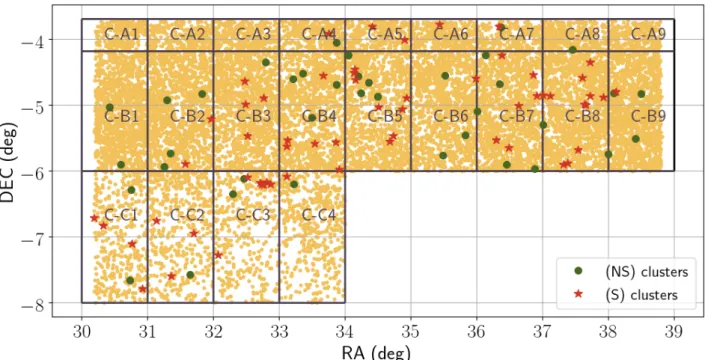
The final galaxy sample is obtained from the crossmatch between the photometric and spectroscopic sample. Figure 2
Fig. 2.Spatial distribution in the XXL-N area of galaxies in the spectrophotometric sample (yellow dots) and of X-ray confirmed clusters. The clusters in superclusters are reprensented with red stars and the clusters outside superclusters with green points. The region is divided into 22 cells (named as indicated inside each cell), used to compute the spectroscopic completeness (see details in AppendixA).
shows the distribution of galaxies and clusters in the coordinates plane, for the magnitude limited sample that is presented below. 2.3. Tools
The stellar population properties of galaxies were derived rely-ing on either their photometric or spectroscopic data. In the first case, we made use of the spectral energy distribution (SED) fitting code LePhare6 (Arnouts et al. 1999; Ilbert et al. 2006) to compute absolute magnitudes, and therefore rest-frame colours, as described in XXL Paper XXII. In the sec-ond case, we fit galaxy spectra via SINOPSIS7 (SImulatiNg
OPtical Spectra wIth Stellar population models), a spectropho-tometric fitting code fully described inFritz et al.(2007,2011, 2017) and already largely used to derive physical properties of galaxies in many samples (Dressler et al. 2009; Vulcani et al. 2015; Guglielmo et al. 2015; Paccagnella et al. 2016, 2017; Poggianti et al. 2017). Among the outputs of the model, we con-sidered SFRs and galaxy stellar masses (M∗), defined as the mass
locked into stars, both those which are still in the nuclear-burning phase, and remnants such as white dwarfs, neutron stars, and stellar black holes.
While LePhare could be applied to the whole spectrophoto-metric sample of galaxies (provided that the catalogue contains magnitudes at least in two filters for each objects), SINOPSIS was run on the subsample of galaxies that have either SDSS or GAMA spectra, which are flux calibrated and have the best avail-able spectral quality. As discussed in Fritz et al.(2014), in the lowest resolution spectra of this work, i.e. GAMA spectra, emis-sion lines can be measured down to a limit of 2 Å, while any emission measurement below this threshold is considered unre-liable. In terms of sSFR, this sets a lower limit of 10−12.5yr−1.
6 http://www.cfht.hawaii.edu/~arnouts/lephare.html 7 http://www.crya.unam.mx/gente/j.fritz/JFhp/SINOPSIS.
html
The final sample is composed of galaxies with reliable out-puts coming from both LePhare and SINOPSIS.
2.4. Samples and spectroscopic completeness
In what follows, we consider galaxies in three redshift bins, 0.1 ≤ z < 0.2, 0.2 ≤ z < 0.3, 0.3 ≤ z ≤ 0.5 and study both magnitude and mass limited samples. As detailed in XXL Paper XXII, magnitude completeness limit was set to an observed magnitude of r= 20.0 at all redshifts, and is converted into a different mass completeness limit at each redshift. To determine this limit, at each redshift we converted the observed magnitude limit into a rest-frame magnitude limit and computed the mass of an ideal object having the faintest magnitude and the reddest colour in that redshift bin. Following XXL Paper XXII, the stellar mass limit of each redshift bin is that corresponding to the lowest limit of each interval; i.e. at 0.1 ≤ z < 0.2 is the stellar mass limit corresponding to z = 0.1. We therefore adopted the following values:
– 0.1 ≤ z < 0.2: M?> 109.5M
– 0.2 ≤ z < 0.3: M?> 1010.3M
– 0.3 ≤ z ≤ 0.5: M?> 1010.8M .
The galaxy magnitude complete sample includes 18 399 galax-ies, the mass complete sample includes 13 857 galaxies. Table2 reports the number of galaxies in the different redshift bins for both samples. Both raw numbers and those corrected for incom-pleteness are given. The method used to compute the spectro-scopic completeness is described in Appendix A. Briefly, as the spectroscopic sample spans a relatively wide redshift range, we sliced the sample into different redshift bins and quanti-fied the number of galaxies that fall/are expected to fall into that given redshift bin, based on both spectroscopic and pho-tometric redshifts. As already performed in XXL Paper XXII, we accounted for the change in the spectroscopic sampling of different surveys by dividing the sky into 22 cells (shown in Fig. 2), and in intervals of 0.5 r-band magnitude within
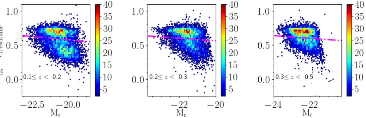
Fig. 3.Colour–magnitude diagrams in the magnitude limited sample in the three redshift bins analysed, with increasing redshift from left to right as indicated in the labels. Single galaxies are plotted as blue dots, while galaxies in higher density regions are grouped together and plotted as rectangles colour-coded according to their number density as indicated in the colour bar located on the side of each panel. The magenta dotted line shows the separation between red and blue objects using the (g − r)rest-framecolour.
each cell. The completeness curves resulting from this com-putation were converted into completeness weights which are attributed to each galaxy given its redshift, astrometry, and magnitude.
3. Galaxy subpopulations
In our analysis we characterised separately the star-forming properties and rest-frame colours of galaxies in different envi-ronments and at different redshifts. We therefore need to define two different criteria to separate star-forming/blue galaxies from passive/red galaxies.
First, we considered as “star forming” those galaxies with sSFR = SFR/M? > 10−12yr−1 and “passive” the remaining galaxies. We point out that this sSFR threshold is the same in the three redshift bins considered, which is justified by the scarce evolution in the sSFR-stellar mass plane in this redshift range (see e.g.Whitaker et al. 2012).
Then, we considered as “blue” galaxies those whose rest-frame colour is bluer than a certain threshold, and “red” the rest. To identify such threshold in colour, we investigated the rela-tion between the (g − r)rest-frame colour and absolute magnitude
Mr, in the three redshift bins separately. Figure3shows the
rest-frame colour–magnitude diagram (CMD) in each redshift bin. To define the slope of the colour–magnitude cut, we focussed on the lowest redshift bin, which has a sufficiently wide magnitude range. We considered five 0.6 absolute magnitude bins and plot the (g − r)rest-framehistogram of each subpopulation (Fig.4). We
then fit the histogram with a double-Gaussian curve and deter-mined the minimum of the distribution between the two peaks. We computed the line interpolating the (g−r)rest-framecolours just
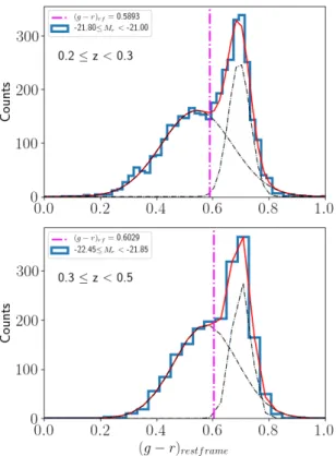
found in the five magnitude bins and used it to divide the galaxy population as shown in Fig.3(magenta dashed line). At higher redshift, the magnitude range is too small to apply the same pro-cedure. As no significant evolution is expected in the slope of the relation, but only in the zero point, we fixed the slope to that of the lowest z bin and computed the appropriate zero points with the same method outlined above (Fig. 5): we considered one magnitude bin at each redshift, we drew the (g − r)rest-frame
colour histogram and fit the distribution with a double-Gaussian curve, finding the local minimum between the two peaks.
To conclude, at 0.1 ≤ z < 0.2 galaxies were assigned to the blue sequence if their colour obeys (g − r)rest-frame< −0.019Mr+
Fig. 4. Rest-frame (g − r) colour distributions in five absolute mag-nitude bins for galaxies at 0.1 ≤ z < 0.2. The red curve shows the double-Gaussian fit performed on the distributions and the single Gaus-sians are represented with the black dashed line. The magenta vertical lines indicate the local minima in the valley between the two Gaus-sian peaks, and define the separation between the red sequence and blue cloud.
0.192, at 0.2 ≤ z < 0.3 the zero point is 0.177 and 0.176 at 0.3 ≤ z ≤ 0.5.
Fig. 5.Rest-frame (g−r) colour distributions performed in one represen-tative absolute magnitude bin in the two highest redshift bins indicated in each panel. Curves and colours are shown as in Fig.4.
As a comparison between the two criteria just described we note that, considering all the redshift bins together, blue galax-ies have a median sSFR ∼ 10−9.7yr−1 (and 90% of galaxies
have sSFR & 10−10.45yr−1). Conversely, star-forming galaxies
have a median (g − r)rest-frame∼ 0.58 (and 90% of galaxies have
(g − r)rest-frame< 0.725).
It is important to bear in mind that the two tracers used to characterise the galaxy populations have a different physi-cal meaning and refer to different timescales. While the SFR is an instantaneous measure of the rate at which a galaxy is form-ing stars at the epoch it is observed, colours are the result of longer processes tracing the predominant stellar population of a galaxy, whose colour is sensitive to its past history and to its cur-rent star formation activity. Moreover, colour is also influenced by other characteristics, such as the metallicity and the pres-ence of dust. In addition, the methodologies adopted to compute SFR and colours are different. The ongoing SFR is a product of the full spectral fitting analysis performed on the spectra, while rest-frame colours are derived by means of SED fitting on the photometry. Therefore, it is important to investigate the two quantities separately and study the incidence of each population over the total, as we do in the next sections.
4. Results I: Galaxy population properties as a function of the global environment
In this section, we study the fractions and star-forming proper-ties of galaxies in different global environments. We consider galaxies in the following environments.
– Cluster virial members are galaxies whose spectroscopic red-shift lies within 3σ from the mean redred-shift of their host clus-ter, where σ is the velocity dispersion of their cluster and whose projected distance from the cluster centre is <1r200.
– Cluster outer members are galaxies whose spectroscopic red-shift lies within 3σ from the mean redred-shift of their host clus-ter, and whose projected distance from the cluster centre is between 1 and 3 r200.
– Galaxies in the field are all galaxies that do not belong to any cluster.
We note that all galaxies belonging to a structure are always included in the same redshift bin. For example, if a cluster is located at the edge of a redshift bin and its members spill over another bin, these are all included in the redshift bin of their host cluster, regardless of their actual redshift.
We also treat separately virial and outer members that belong or do not belong to a supercluster.
Table3reports the number of galaxies in the different envi-ronments and redshift bins. For all of these subsamples, numbers are given for the magnitude limited and mass limited samples. At 0.1 ≤ z < 0.2 our sample includes three superclusters, at 0.2 ≤ z < 0.3 three superclusters, and at 0.3 ≤ z ≤ 0.5 six superclusters.
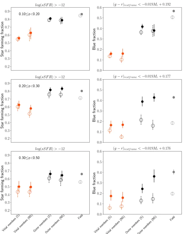
4.1. Fraction of blue and star-forming galaxies
Figure6 shows the fraction of blue and star-forming galaxies, separately, in the different global environments and in the three redshift bins, both for the magnitude limited and mass limited samples. Error bars are computed using a bootstrap method. For galaxies in the field, we include in the error budget both the bootstrap error and the uncertainty due to the cosmic variance. FollowingMarchesini et al.(2009), we sliced our field into nine right ascension subregions and we computed the fraction of star-forming and blue galaxies of each region separately; the con-tribution to the error budget from cosmic variance is then the standard deviation of the newly computed fractions divided by the number of subregions considered.
Overall, at all redshifts, both considering the star formation and colours as tracers, fractions are similar within and outside the superclusters, suggesting that neither additional quenching processes nor triggering of the star formation are associated with the presence of superclusters.
At 0.1 ≤ z < 0.2 (top left), both in the magnitude and in the mass limited samples, the star-forming fraction strongly depends on environment. Virial members have the lowest fraction of star-forming galaxies (55–60%). This fraction increases when considering outer members, where ∼80% of galaxies are star forming. Finally, the percentage of star-forming galaxies in the field is the highest (86 ± 1%). The same trends are recovered when considering galaxy colours, even though fractions are sys-tematically lower: ∼16% of virial members are blue, as are ∼40% of outer members and 57% of field galaxies. Similarly to the star-forming fractions, results in the magnitude and mass limited samples are similar, except for the field value, where they differ by ∼10%; the mass limited sample shows a lower fraction than the magnitude-limited sample.
At 0.2 ≤ z < 0.3 (middle panels of Fig.6), in both samples, virial members still show a significantly lower fraction of star-forming galaxies than the other environments (∼55−60%), while outer members and field galaxies present very similar fractions (∼85%/75% in the magnitude/mass limited samples). Consider-ing colour fractions, the same trends are detected in the mag-nitude limited sample, where blue galaxies are ∼17% in virial members, ∼42% in outer members and in the field. In the mass limited samples, the difference between outer members and the field is much smaller: the fraction of blue galaxies in these envi-ronments is always <20%.
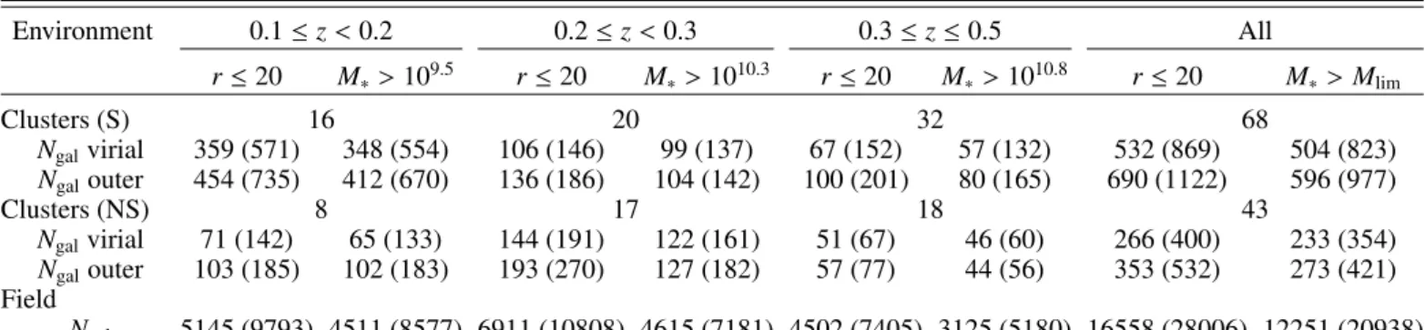
Table 3. Number of galaxies in the different environments (clusters in superclusters (S), clusters not in superclusters (NS), and field) and above the magnitude and mass completeness limits, in three redshift bins.
Environment 0.1 ≤ z < 0.2 0.2 ≤ z < 0.3 0.3 ≤ z ≤ 0.5 All r ≤20 M∗> 109.5 r ≤20 M∗> 1010.3 r ≤20 M∗> 1010.8 r ≤20 M∗> Mlim Clusters (S) 16 20 32 68 Ngalvirial 359 (571) 348 (554) 106 (146) 99 (137) 67 (152) 57 (132) 532 (869) 504 (823) Ngalouter 454 (735) 412 (670) 136 (186) 104 (142) 100 (201) 80 (165) 690 (1122) 596 (977) Clusters (NS) 8 17 18 43 Ngalvirial 71 (142) 65 (133) 144 (191) 122 (161) 51 (67) 46 (60) 266 (400) 233 (354) Ngalouter 103 (185) 102 (183) 193 (270) 127 (182) 57 (77) 44 (56) 353 (532) 273 (421) Field Ngal 5145 (9793) 4511 (8577) 6911 (10808) 4615 (7181) 4502 (7405) 3125 (5180) 16558 (28006) 12251 (20938)
Notes. Galaxies in clusters are further subdivided into virial and outer members. The quantities in parentheses refer to the number of galaxies weighted for spectroscopic completeness.
We recall that this redshift bin contains the XLSSsC N01 supercluster, separately discussed in XXL Paper XXX, and that contributes to the (S) cluster population with 11 out of 20 clus-ters, corresponding to ∼65% of the cluster population. In that supercluster an enhancement of the star formation activity of outer members with respect to the virial population and the field was observed. Nonetheless, general trends are maintained within the errors.
At 0.3 ≤ z ≤ 0.5 (bottom panels of Fig.6), both in the mass and magnitude limited samples, virial members have the lowest star-forming fraction (45–50%), but differences with the other environments are reduced: in outer members and in the field the star-forming fractions are ∼65% in the magnitude limited sample and ∼55−60% in the mass limited sample. Considering colours, in the magnitude limited sample we still detect the usual dif-ferences between virial members and galaxies in other environ-ments, while in the mass limited sample all fractions are lower than 15% and no variation with environment is detected.
As our cluster sample spans a wide range of X-ray luminos-ity (see Fig.1), we repeat the analysis separating the clusters in bins of X-ray luminosity, but find no significant additional trends (plot not shown).
To summarise, at all redshifts, field galaxies have the high-est incidence of star-forming/blue galaxies, while virial members exhibit a noticeable suppression of both star-forming and blue fractions with respect to the other environments. Outer members exhibit a significant suppression of the star-forming/blue frac-tions with respect to the field only at 0.1 ≤ z < 0.2, while at higher redshift they present similar fractions. No significant dif-ferences are detected between galaxies within and outside super-clusters. However, fractional differences within and outside of superclusters do not follow a common trend at all redshifts, likely reflecting the variation of properties of individual supercluster structures at different redshifts. The choice of a mass or magni-tude limited sample only marginally affects the star-forming frac-tions, while it strongly alters those based on colours at z > 0.2.
Overall, star-forming and blue fractions are never consistent within the errors: this is a probe that the two quantities, even though strictly related, are actually reflecting different aspects of the evolution of the galaxies. We note that in our sample no reasonable and physically motivated cut could be adopted to rec-oncile the fractions of star-forming and blue galaxies.
In principle, the difference in the star-forming and blue frac-tions could be due to the presence of AGNs; for example, low-ionisation nuclear emission-line regions (LINERS) identified as
red star-forming galaxies. These AGNs would increase the num-ber of galaxies pertaining to the star-forming population with-out enhancing the fraction of blue galaxies. To test this, we removed broad- and narrow- line AGNs from our galaxy sample, as described in detail in AppendixB, and we computed again the star-forming/blue fractions. The fractions are substantially unchanged (plot not shown), indicating that our results are not driven by the possible presence of AGNs.
We stress that comparisons across the different redshift bins are not possible, as magnitude and mass values used to define the sample are different. Furthermore, we point out that the decrease of the blue/star-forming fraction with increasing redshift is sim-ply an artefact due to the galaxy mass range probed at different redshifts.
4.2. SFR–mass relation
We focus in this section only on the star-forming population and investigate the correlation between the SFR and galaxy stellar mass (SFR–M?). For this analysis we only rely on the mass limited sample. Indeed, in contrast with the magnitude lim-ited sample, applying a mass limit ensures completeness, i.e. to include all galaxies more massive than the limit regardless of their colour or morphological type. This ensures that we do not bias the results because of the absence of galaxies which are under-sampled or missed by selection effects, as might happen when considering a magnitude limited sample. As in the previ-ous section we did not detect any significant difference between galaxies within and outside superclusters, in what follows we do not distinguish between the two subgroups.
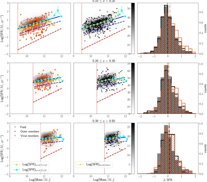
Figure 7 compares the distribution of galaxies in di ffer-ent environmffer-ents and in different redshift bins in the SFR–M?
plane (left and middle panels). Roughly, at all redshifts, galaxies located in the different environments share a common region on the plane, excluding strong environmental effects at play. Com-paring the galaxies at different redshifts, we find a decline in SFR with time at fixed stellar mass, in agreement with many previous literature results (e.g.Noeske et al. 2007;Vulcani et al. 2010).
To probe the apparent lack of environmental effects on a sta-tistical ground, we proceed by first performing a linear regression fit to the relation by considering all the different environments together and then compare the median values of SFR in different mass bins for the various environments to this fit. The values of the best-fit slope, intercept and 1σ are given in Table5. Error bars on the medians are computed in each stellar mass bin as 1.253σ/√n,
Fig. 6.Fraction of star-forming (left) and blue (right) galaxies in different environments and different redshifts, as indicated in the panels. Cluster
members are divided into four subsamples: virial and outer members that belong or do not belong to a supercluster. Values obtained using the magnitude limited sample are represented with filled symbols and solid errors, those obtained using the mass limited sample are represented by empty symbols and dashed error bars. A horizontal shift is applied for the sake of clarity. Errors are derived by means of a bootstrap method.
where σ is the standard deviation of the SFR distribution in the bin and n is the number of objects considered in the bin.
The fit to the SFR–M?relation is dominated by field
galax-ies, whose median trends closely follow the fitting line at all redshifts. In contrast, cluster virial members show hints of lower median SFR with respect to the latter in all the redshift bins; some statistical oscillations are due to the lower number of galaxies at 0.3 ≤ z ≤ 0.5. Furthermore, in this case the limited
mass range could also affect the reliability of the fit. The median SFR of outer members closely follows the field trend at z ≤ 0.2 and is compatible within the error bars with both the field and virial members at higher redshift. We do not plot these values for the sake of clarity.
The right-hand panels of Fig. 7 report the distribution of the differences between the SFR of each galaxy and the value derived from the global fit given the galaxy mass (∆SFR), for
Fig. 7.Left and middle panels: SFR–M?relation for galaxies in the field and cluster virial and outer members (grey 2D histogram and density
contours, orange diamonds, and black stars, respectively) in the mass limited sample. Panels in different lines refer to different redshift bins. The field population is represented with a 2D histogram whose values are given in the colour bar included in the middle panel, and grey contours trace the density levels of the data points. The vertical red dashed line shows the stellar mass limit at each redshift, while the oblique red dashed line sets the limit to the star-forming population, i.e. sSFR= 10−12yr−1. The blue line is the linear fit to the SFR–M
?relation including all the
environments at each redshift, and the dashed blue lines correspond to 1σ errors on the fitting line. The parameters of the fit and the values of σ are given in Table5. The gold diamonds/stars and cyan dots represent the median SFR values computed in mass bins of 0.2 dex width, for the
virial/outer members and field population, respectively. Error bars on the medians are computed assuming a normal distribution of the data points as 1.253σ/√n, where σ is the standard deviation of the distribution and n is the number of objects in the considered stellar mass bin. Right panels: histograms of the differences between the expected SFR computed using the main sequence fitting line at the stellar mass of any given galaxy in our sample and its actual SFR (∆SFR). Positive values of ∆SFR indicate reduced SFR compared to the SFR main sequence of star-forming galaxies. The median values of the distributions are also shown with vertical dashed lines and different environments are colour coded as written in the legend.
any given environment. Positive values of∆SFR correspond to reduced SFR with respect to the expected value. At all red-shifts, it is immediately clear that the shape of distribution of ∆SFR of virial members differs from that of the field population, whereby the former presents a tail of reduced SFR values with respect to the latter. A Kolmogorov–Smirnov (KS) test is able to detect differences between virial members and field galaxies at all redshifts (P(KS) ≤ 0.05); outer members instead have sta-tistically different distributions with respect to the field only at 0.3 ≤ z ≤ 0.5 (P(KS) < 0.02), and with respect to virial
mem-bers only at 0.1 ≤ z < 0.2 (P(KS) < 10−3). Nonetheless, at all
redshifts, median values are compatible within the errors among the different samples, indicating that the tail, although present in virial and outer members, is not able to affect the whole SFR distribution significantly.
4.3. Galaxies in transition
The presence of a non-negligible number of galaxies with reduced SFR among the cluster population motivates a more
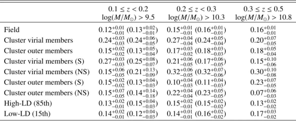
Table 4. Fraction of galaxies in transition in different environments in the three redshift bins.
0.1 ≤ z < 0.2 0.2 ≤ z < 0.3 0.3 ≤ z ≤ 0.5 log(M/M ) > 9.5 log(M/M ) > 10.3 log(M/M ) > 10.8
Field 0.12+0.01−0.01(0.13+0.02−0.01) 0.15+0.01−0.01(0.16+0.01−0.01) 0.16+0.01−0.01 Cluster virial members 0.24+0.03−0.03(0.24+0.06−0.05) 0.27+0.04−0.04(0.24+0.05−0.04) 0.20+0.07−0.05 Cluster outer members 0.15+0.02−0.02(0.13+0.05−0.04) 0.17+0.03−0.02(0.18+0.03−0.03) 0.18+0.05−0.04 Cluster virial members (S) 0.27+0.03−0.03(0.25+0.08−0.07) 0.21+0.06−0.05(0.17+0.06−0.05) 0.15+0.10−0.06 Cluster virial members (NS) 0.15+0.06−0.05(0.21+0.13−0.09) 0.32+0.06−0.05(0.32+0.07−0.06) 0.30+0.10−0.08 Cluster outer members (S) 0.15+0.02−0.02(0.13+0.04−0.03) 0.10+0.04−0.03(0.11+0.04−0.03) 0.23+0.07−0.05 Cluster outer members (NS) 0.15+0.07−0.05(0.14+0.14−0.18) 0.22+0.04−0.04(0.23+0.05−0.05) 0.07+0.06−0.03 High-LD (85th) 0.13+0.02−0.01(0.15+0.04−0.03) 0.15+0.02−0.01(0.15+0.02−0.02) 0.13+0.02−0.02 Low-LD (15th) 0.14+0.02−0.01(0.12+0.04−0.03) 0.14+0.01−0.01(0.16+0.02−0.02) 0.17+0.03−0.02
Notes. Numbers are weighted for spectroscopic incompleteness and are computed above the stellar mass completeness limit of each redshift bin; the values in parenthesis refer to the highest stellar mass limit to allow comparisons at different redshifts. Errors are computed by means of bootstrapping. The last two lines of the table correspond to the values computed in two bins of LD and are analysed in Sect.5.
Table 5. Best-fit parameters of the linear fit to the SFR–M? relations shown in Fig.7, in three redshift bins.
a b σ
0.1 ≤ z < 0.2 0.61 −5.86 0.59 0.2 ≤ z < 0.3 0.35 −2.92 0.52 0.3 ≤ z < 0.5 0.22 −1.31 0.48
Notes. The fit is performed on the sample including all the environ-ments together, and the fitting line has the following general equation: Log(SFR)= aLog(M?)+ b.
detailed investigation on the presence of the so-called galax-ies in transition, i.e. star-forming galaxgalax-ies which are slowly decreasing their SFR and are detected as an intermediate pop-ulation migrating from the star-forming main sequence down to the quenched population. To identify the galaxies in transi-tion we followPaccagnella et al.(2016), and select galaxies with (sSFR) > 10−12yr−1and SFR below 1σ from the SFR–M? fit-ting line. The transition fraction is computed as the ratio of this population to the number of star-forming galaxies in each envi-ronment. We note that, by definition, the percentage of galaxies below a 1σ cut of the SFR–M? relation should be ∼15–17%,
therefore the identification of a population of galaxies in transi-tion is measured as an excess of galaxies compared to this statis-tical value.
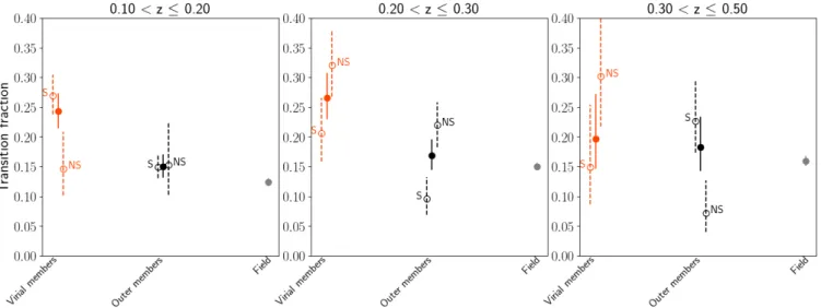
The fractions of galaxies in transition as a function of environment for different redshift bins are presented in Fig.8 and given in Table 4. We compute these fractions also divid-ing virial/outer cluster members residing or not in super-clusters.
The incidence of the population of galaxies in transition depends on environment. As shown in Fig. 8, the fraction of transition galaxies in the field and outer members is (within the errors) almost half of that observed in cluster virial members at z ≤ 0.3. At higher redshift instead, the fractions are simi-lar within the error bars in all environments, likely owing to the high stellar mass limit considered.
Considering separately clusters within and outside super-clusters, no clear trends are observed in the transition fractions, suggesting again that differences among superclusters are most
likely statistical. In this context, we note that at 0.2 ≤ z < 0.3 the fraction of galaxies in transition in the virial and outer regions of (S) clusters is in agreement with the trends found for the XLSSsC N01 supercluster (XXL Paper XXX). The transition fractions are ∼10% lower in both (S) virial and outer members compared to their (NS) counterparts, as in the XLSSsC N01 supercluster where the percentage of galaxies with reduced SFR was <20% in all the environments.
We also tested whether the X-ray luminosity played a role in the determination of the number of galaxies in transition in clus-ters, and we did not find any clear correlation in the luminosity range probed by our cluster sample.
As a general understanding, environmental effects seem to dominate within the cluster virial radii: the substantial di ffer-ence in the number of galaxies with reduced SFR among cluster virial members compared to the field population is responsible for detection of tails in the∆SFR distributions, shown in the right panels of Fig.7.
5. Results II: Galaxy population properties as a function of the local environment
The availability of a large spectrophotometric sample of galax-ies enables the parametrisation of environment also in terms of projected LD of galaxies. In this section we consider together the galaxies in all the aforementioned environments and divide these sources into the usual three redshift bins. For each galaxy, we compute the projected LD as the number of galaxies enclosed into a fixed radial aperture of 1 Mpc at the redshift of the galaxy and within a given redshift range around the centre galaxy. We describe the computation of LD in detail in AppendixC. Figure9 shows the LD distribution in the three redshift bins in logarith-mic units, along with the 15th, 50th, and 85th percentiles, which will be used to define the LD bins used in Sect.5.2. It is evident that going from low- to high-z the peak (i.e. the median) of the LD is shifted towards higher densities, as previously found in other samples (Poggianti et al. 2010).
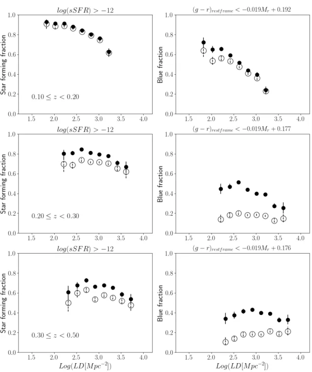
5.1. Fraction of blue and star-forming galaxies
Figure 10 shows the fraction of blue (right) and star-forming (left) galaxies as a function of the projected LD, in the three
Fig. 8. Fraction of galaxies in transition in the mass limited sample in the three redshift bins. Filled dots represent galaxies in the different environments, as written in the x-axis. The (S) and (NS) contribution to the virial and outer member populations are also represented with empty symbols and dashed error bars. Error bars are computed via bootstrapping.
Fig. 9.Distributions of the logarithm of the LD in the three redshift bins, as indicated in the labels. Histograms are drawn after a sigma-clipping has been performed on the parent distributions. The red dashed vertical lines represent the 15th, 50th and 85th percentiles, respectively.
redshift bins, separately, for both the magnitude and mass lim-ited samples. Error are derived by means of bootstrapping.
At 0.1 ≤ z < 0.2 (top panels), both in the magnitude and in the mass limited samples, the fraction of both star-forming and blue galaxies decreases monotonically with increasing LD. The star-forming fraction is close to 90% at low densities and then decreases of a factor &1.5 in a LD range of 2.0 dex; the blue fraction is ∼80% at low densities and decreases of almost four times; the values drop to ∼0.2 at the highest densities.
At 0.2 ≤ z < 0.3 (middle panels of Fig.10), the star-forming fractions are much less dependent on density, both in the mass and magnitude limited samples. Values range between 80 and 60%, at low and high density, respectively. In contrast, in the magnitude limited sample, the blue fraction still shows a signif-icant decrease with LD, ranging from 50% at low densities to 20% at the highest. In the mass limited sample the blue fraction is always.20%, regardless of density.
In the highest redshift bin (bottom panels of Fig.10), both in the magnitude and mass limited samples the star-forming frac-tions seem first to increase with density, reach a plateau and then decrease at the highest values. Overall, values range between 50
and 70% in the magnitude limited sample, 40% to 60% in the mass limited sample. Such increase with LD is also noticeable in the colour fractions: in the magnitude limited sample at low density the fraction is ∼25%, reaches 40% at intermediate den-sities and falls down to 30% at the highest density. In the mass limited sample, the fraction of blue galaxies is always <20%, but shows a statistically meaningful increase from the lowest to the highest densities.
To summarise, the star-forming/blue fraction of galaxies decreases at densities higher than the LD median at each red-shift (see Fig.9). At densities lower than the median, we notice a steady decrease of the fractions at 0.1 ≤ z < 0.2, opposed to an initial increase at z ≥ 0.2. Furthermore, the overall decrease of the star-forming/blue fractions going from the low to high densities is much more pronounced at lower than at higher red-shifts. As it was previously found in Sect.4.1, considering either the magnitude limited sample or the mass limited sample lead to substantial differences only in the fraction of blue galaxies at z > 0.2. Finally, differences in the absolute values of star-forming and blue fractions are again noticeable and are further investigated and discussed in Sect.6.2.
Fig. 10.Fraction of star-forming galaxies in different bins of LD, computed with the sSFR (left panels) and rest-frame colour (right panels).
Three redshift bins from z= 0.1 up to z = 0.5 are represented, and the redshift increases from top to bottom panels as indicated in each panel. A sigma-clipping has been performed on the parent LD distributions to remove outliers and bins with a non-statistically representative number of objects. Panels and symbols are shown as in Fig.6.
5.2. SFR–mass relation and galaxies in transition
We now study the SFR–M? relation of galaxies in two extreme
bins of LD representative of the lowest and highest LD environ-ments. With reference to the histrograms represented in Fig.9, we selected two percentiles that allowed us to seize the wings of the distribution (having previously removed outliers), consider-ing its narrow shape. The selected percentiles are 15th and 85th. In Fig.11we report the SFR–M?relation of galaxies in the
low- and high-LD regimes. We proceed as before and compute the median SFR in stellar mass bins of 0.2 dex width in the low-and high-LD regimes. The median values of the SFR computed
in bins of stellar mass show little variation with LD (yellow diamonds versus cyan stars), whose values that are always con-sistent within the error bars. Differences arising at the highest stellar mass values at z ≥ 0.3 may be mostly driven by the low sample statistics, and therefore should be taken with caution. The right-hand panels of Fig.11show the∆SFR with respect to lin-ear fit to the SFR–M? relation used in Sect. 4.2, computed as previously done for the global environment. The median∆SFR values are very similar in the high- and low-LD regimes at all redshifts, and the statistical similarity between the two samples is further confirmed by the outcome of the KS test: P(KS) 0.05 at all redshifts.
Fig. 11.Left panels: SFR–M?relation for galaxies in two regimes of LD, corresponding to the wings of the LD histograms shown in Fig.9. Panels
and lines are shown as Fig.7. Cyan stars and the gold diamonds represent the median values of the SFR computed in 0.2 dex stellar mass bins, for the low- and high-LD regimes respectively. Error bars are computed as in Fig.7. Right panels: histograms of the differences between the expected SFR computed using the main sequence fitting line at the stellar mass of any given galaxy in our sample and its actual SFR (∆SFR). Median values of the distributions are shown with vertical dashed lines and colour coded as written in the legend.
Finally, we also compute the fraction of transition galaxies in the two extreme LD bins (see Table4), finding no differences within the error, at all redshifts.
6. Discussion
In this paper we have adopted two definitions of environment. The first is based on the X-ray selection of virialised structures; the second is based on the local galaxy number density. We are now in the position of contrasting the results, and we aim to
understand whether the different parametrisations lead to simi-lar conclusions.
In the literature, the environmental dependence of the galaxy properties was previously investigated by many authors, adopt-ing either a global or local parametrisation, but hardly ever directly contrasting the two in homogeneous samples. Nonethe-less, as discussed by Vulcani et al. (2011, 2012, 2013) and Calvi et al. (2018), the two definitions are not interchangeable and can give opposite results, highlighting that different pro-cesses dominate at the different scales probed by the different definitions.
As far as galaxy fractions are concerned, we find that regardless of the environmental definition adopted the frac-tion of blue/star-forming galaxies is systematically higher in the field/least dense regions than in the virial regions of clus-ters/highest densities. This effect is less significant in the high-est redshift bin analysed. Our results are overall in line with what was previously found in the literature, both considering the global (e.g.Iovino et al. 2010;Muzzin et al. 2012) and local (e.g. Balogh et al. 2004b; Cucciati et al. 2017) environments. Similarly, the overall SFR–M?relation also seems not to depend on the parametrisation adopted, which agrees with numerous lit-erature results that claim the invariance of SFR–M?relation on
environment (e.g.Peng et al. 2010).
Nonetheless, the two definitions of environment lead to different results when we analysed the fraction of galaxies in transition. In fact, using the local environment the fraction of galaxies below the main sequence is similar at low and high den-sity, whereas in clusters (and especially in their virial regions) a population with reduced SFR with respect to the field is observed. This population is most likely in a transition phase of star formation and, although clearly detected, it is not able to affect the whole SFR–M?relation because it constitutes a small fraction of all galaxies, as shown in Table4.
6.1. Galaxies in transition in the different environments and their evolution with redshift
The presence of a population of galaxies in transition from being star forming to passive was already detected in galaxy clusters by several works at low and intermediate redshifts (Patel et al. 2009;Vulcani et al. 2010;Paccagnella et al. 2016), and has been interpreted as an evidence for a slow quenching process prevent-ing a sudden relocation of galaxies from the star formprevent-ing to the red sequence.
In the previous sections, it was not possible to investigate the evolution of the incidence of transition galaxies, as a dif-ferent mass complete limit was adopted at each redshift. Now we consider instead the same mass limit, to allow for fair com-parisons. We adopt the most conservative value, that is the mass completeness limit in the highest redshift bin. Fractions are given in parenthesis in Table4.
Figure12shows the fraction of galaxies in transition in the redshift range 0.1 ≤ z ≤ 0.5 considering the global and local environments.
The upper panel shows that in the case of global environment the overall fraction of transition galaxies with log(M?/M ) >
10.8 does not significantly vary with cosmic time, remaining around ∼15%, both in the field and among outer members. In contrast, virial members present higher transition fractions with a tentative increase as time goes by, although uncertainties pre-vent us from drawing solid conclusions.
The same figure also compares our results to those obtained at low redshift (z . 0.1) byPaccagnella et al.(2016), when the subsample of their cluster galaxies within 1r200and with stellar
masses M? ≥ 1010.8M is considered. The resulting transition
fraction weighted for incompleteness is 0.30+0.04−0.03, that is consis-tent with our results within the error bars and point towards the aforementioned increase in the transition fractions at more recent epochs.
In contrast, the lower panel of Fig. 12 shows no depen-dence of the transition fraction with redshift for galaxies located at different local densities, further demonstrating that the local environment does not affect the incidence of such population.
Fig. 12.Fraction of galaxies in transition at 0.1 ≤ z ≤ 0.5 consider-ing the global (top) and local (bottom) parametrisation Fractions are computed for log M/M ≥ 10.8, the stellar mass completeness limit
at 0.3 ≤ z ≤ 0.5. Error bars on the fractions are computed via boot-strapping. In the top panel, the blue star represents the fraction of transition galaxies in the local universe, adapted fromPaccagnella et al.
(2016).
Evidently, the two parametrisations are able to probe dif-ferent physical conditions for galaxies, determining di ffer-ent timescales in the star formation process and quenching timescales.
6.2. Star-forming versus colour fractions in the different environments
In the previous sections we have separately analysed the depen-dence of the star-forming and blue galaxy fractions on the global and local environments. In both analyses a difference between the star-forming and blue fractions emerged, wherein the for-mer is systematically higher than the latter. We stress that this difference is not likely to be due to the definition we adopted for determining the two populations: as previously described in Sect.3, the sSFR and colour threshold adopted for defining the
Fig. 13. Ratio of the fraction of star-forming (FSFing) to blue (Fblue)
galaxies in the mass limited sample in the three redshift bins and in different global (top) and local (bottom) environments. Dashed lines in the top panel show trends when AGNs are removed form the sample as explained in the AppendixB. In both panels, error bars are computed by propagating the asymmetric errors on the single fractions by means of the statistical error propagation.
star-forming and blue populations are physically motivated by the distribution of the galaxy samples in the sSFR–M? plane and by the rest-frame colour distribution at different redshifts. We further explored whether a choice of different cuts either on the sSFR and on the (g − r) rest-frame colour led to more similar galaxy fractions and concluded that the resulting sSFR and/or colour threshold to apply to the population in order to reconcile the fractions were totally non-physical.
As already anticipated in Sect.3, the two quantities present intrinsic differences related to the tracers they are based on: the SFR is derived from the measure of the flux of emission lines sensitive to the short-lived massive stars, while avoiding as much as possible contributions from evolved stellar popu-lations. It is basically able to probe the presence of newly or recently formed stars on timescales of ∼10–100 Myr. On the contrary, galaxy integrated colours are more sensitive to the inte-grated star formation history and in particular to the stellar pop-ulations dominating the galaxy light, and are further influenced by the dust content and metallicity of the galaxy. With this in mind, we can expect a good agreement between galaxy rest-frame colours and SFR indicators when the galaxy is actively forming stars at a steady rate on the main sequence or, con-versely, when it is quiescent and has been passively evolving for some Gigayear. Differences between the two tracers may
be expected for example when the galaxy suddenly interrupts its star formation activity as a consequence of the interactions with external physical mechanisms (e.g. environmentally related phenomena).
We are now in the position of directly comparing the frac-tion of star-forming and blue galaxies with the intent of obtain-ing some clues regardobtain-ing the physical processes occurrobtain-ing in the different environments.
Figure13shows the ratio of the number of star forming to that of blue galaxies as a function of global (top panel) and local (bottom panel) environment, above the stellar mass complete-ness limit of each redshift bin. In the upper panel of the figure, a strong dependence of the FSFing/Fblueratio on the global
envi-ronment emerges. At 0.1 ≤ z ≤ 0.3, this ratio is highest in the virial regions of clusters, while it decreases in the other environ-ments with little difference found between cluster outskirts and the field. Moving towards higher redshift, uncertainties prevent us from drawing solid conclusions, but still a hint of a higher FSFing/Fblueratio within the virial radii of clusters than the other
environments is visible.
In principle, this result might be contaminated by the pres-ence of AGNs, and in particular LINERS, that could be misclas-sified as red star-forming galaxies. The dashed lines in Fig.13 show the FSFing/Fblueratios after AGNs have been removed (see
AppendixB) and that this population cannot be responsible for the observed trends.
Our results suggest that in the innermost regions of clus-ters, besides the suppression of the star formation activity, fur-ther environmentally related physical processes come into play to produce a population of galaxies with a non-negligible SFR that however is not coupled with (blue) rest-frame colours.
This decoupling is most likely due to the different star for-mation histories that characterise galaxies in the different global environments. Indeed,Guglielmo et al.(2015) found that the star formation history of low-redshift star-forming galaxies has been decreasing since z ∼ 2, and in particular the rate at which stars were produced in galaxies in clusters at high-z is higher than in the field, regardless of their stellar mass. This implies that, on average, star-forming galaxies in clusters formed the bulk of their stellar mass at older epochs than their counterparts in the field. Thus these star forming galaxies host older stellar popula-tions which have redder colours, although these galaxies still are forming stars at the epoch of observation.
Alternatively, the presence of a population of red star-forming galaxies may be also associated with a dust obscured star formation phase.Gallazzi et al.(2009) quantified that nearly 40% of the star-forming galaxies in a supercluster at z ∼ 0.17 (Abell 901/902) had red optical colours at intermediate and high densities. These red systems have sSFR similar to or lower than blue star-forming galaxies, thus they are likely undergoing gen-tle mechanisms that perturb the distribution of gas inducing star formation (but not a starburst) and at the same time increase the gas/dust column density.
The incidence of the red star forming population is instead less dependent on the local environment: the lower panel of Fig.13shows no strong trends of the FSFing/Fblueratio with LD
at any redshift, also because of the large uncertainties, especially at higher redshifts.
These tre nds prove, once again, that the two environmental parametrisations are probing galaxies in different physical condi-tions, and that they cannot be used interchangeably. Indeed, there is no constant direct correspondence between the cluster cores and the highest LD regions and, similarly, between the lowest LD regions and the field.