HAL Id: hal-01217654
https://hal.inria.fr/hal-01217654
Submitted on 20 Oct 2015
HAL is a multi-disciplinary open access
archive for the deposit and dissemination of sci-entific research documents, whether they are pub-lished or not. The documents may come from teaching and research institutions in France or abroad, or from public or private research centers.
L’archive ouverte pluridisciplinaire HAL, est destinée au dépôt et à la diffusion de documents scientifiques de niveau recherche, publiés ou non, émanant des établissements d’enseignement et de recherche français ou étrangers, des laboratoires publics ou privés.
Model with Application in Statistical Modeling of
High-Resolution SAR Images
Heng-Chao Li, Vladimir A. Krylov, Ping-Zhi Fan, Josiane Zerubia, William J.
Emery
To cite this version:
Heng-Chao Li, Vladimir A. Krylov, Ping-Zhi Fan, Josiane Zerubia, William J. Emery. Unsupervised Learning of Generalized Gamma Mixture Model with Application in Statistical Modeling of High-Resolution SAR Images. IEEE Transactions on Geoscience and Remote Sensing, Institute of Electrical and Electronics Engineers, 2016, 54 (4), pp.2153-2170. �hal-01217654�
Unsupervised Learning of Generalized Gamma
Mixture Model with Application in Statistical
Modeling of High-Resolution SAR Images
Heng-Chao Li, Senior Member, IEEE, Vladimir A. Krylov, Ping-Zhi Fan, Fellow, IEEE, Josiane Zerubia, Fellow, IEEE, and William J. Emery, Fellow, IEEE
Abstract
The accurate statistical modeling of synthetic aperture radar (SAR) images is a crucial problem in the context of effective SAR image processing, interpretation and application. In this paper a semi-parametric approach is designed within the framework of finite mixture models based on the generalized Gamma distribution (GΓD) in view of its flexibility and compact form. Specifically, we develop a generalized Gamma mixture model (GΓMM) to implement an effective statistical analysis of high-resolution SAR images and prove the identifiability of such mixtures. A low-complexity unsupervised estimation method is derived by combining the proposed histogram-based expectation-conditional maximization (ECM) algorithm and the Figueiredo-Jain algorithm. This results in a numerical maximum likelihood (ML) estimator that can simultaneously determine the ML estimates of component parameters and the optimal number of mixture components. Finally, the state-of-the-art performance of this proposed method is verified by experiments with a wide range of high-resolution SAR images.
Index Terms
Synthetic aperture radar (SAR) images, finite mixture model, generalized Gamma distribution, expectation-conditional maximization (ECM) algorithm, minimum message length (MML), probability density function estima-tion, unsupervised learning.
I. INTRODUCTION
S
YNTHETIC aperture radar (SAR) has become a very important Earth observation technique because of its all-weather, day-and-night, high spatial resolution and subsurface imaging capabilities [1]. As an active imaging system, SAR generates acquisitions via an imaging algorithm over the received echo signals from interactions of electromagnetic waves emitted by the antenna system of sensor with the illuminated ground area. With the rapid advancement of SAR technologies, such imagery is becoming more accessible, further greatly promoting the potential of SAR applications. In the context of SAR image processing and applications, a crucial problem is represented by the need to develop accurate models for the statistics of pixel intensities. To date, a lot of work related to the statistical nature of SAR images has been published in the literature.From a methodological point of view, the strategies of statistical analysis for SAR images can be divided into three categories: non-parametric, semi-parametric and parametric approaches [2]. The non-parametric approach (e.g., Parzen window, support vector machine) is completely data driven but typically computationally expensive [3]. On the other hand, the parametric approach has the substantial advantages of simplicity and applicability. Given a
This version of the manuscript was accepted to the IEEE Transactions on Geoscience and Remote Sensing on October 9, 2015. This work was supported in part by the Program for New Century Excellent Talents in University under Grant NCET-11-0711, by the National Natural Science Foundation of China under Grant 61371165, by the Innovative Intelligence Base Project (111 Project No. 111-2-14), and by the Fundamental Research Funds for the Central Universities under Grant SWJTU12CX004.
H.-C. Li and P.-Z. Fan are with the Sichuan Provincial Key Laboratory of Information Coding and Transmission, Southwest Jiaotong University, Chengdu 610031, China (e-mail: lihengchao 78@163.com). Now H.-C. Li is also with the Department of Aerospace Engineering Sciences, University of Colorado, Boulder, CO 80309 USA.
V. A. Krylov has participated in the work during his postdoc at the Ayin team, INRIA. He is currently with Dept. of Electrical, Electronic, Telecom. Engineering and Naval Architect. (DITEN), University of Genoa, 16145, Genoa, Italy (e-mail: vladimir.krylov@unige.it).
J. Zerubia is with Ayin research team, INRIA, Sophia Antipolis F-06902, France (e-mail: josiane.zerubia@inria.fr).
W.-J. Emery is with the Department of Aerospace Engineering Sciences, University of Colorado, Boulder, CO 80309 USA (e-mail: emery@colorado.edu).
mathematical model, it formulates the probability density function (PDF) estimation as a parameter estimation problem. The well-known examples in this category include the log-normal [1], Weibull [1], Fisher [4], and generalized Gamma [5] empirical models as well as several theoretical ones, such as Rayleigh [1], Nakagami-Gamma [1], [6], heavy-tailed Rayleigh [7], generalized Gaussian Rayleigh (GGR) [8], generalized Nakagami-Gamma Rayleigh (GΓR) [2], K [9] and G [10]. Nowadays, the new generation of high-resolution spaceborne SAR satellites like TerraSAR-X, COSMO-SkyMed, and RADARSAT-2, together with modern airborne SAR systems, enables the systematic acquisition of data with spatial resolutions reaching metric/submetric values. Increasing SAR resolution implies a reduction of the number of scatterers per resolution cell and also an enhancement of the appreciability of backscattering responses from distinct ground cover materials. Therefore, the histograms of high-resolution SAR images, that commonly contain complex land-cover typologies, exhibit heavy-tailed or bi/multimodal characteristics. Under such conditions, it is impossible to apply a single parametric PDF model to accurately describe the statistics. To address this issue, the semi-parametric approach is a good choice, which is designed as a compromise between nonparametric and parametric ones, and is related to the finite mixture model (FMM) [11] in the sense that the underlying PDF is defined as a weighted sum of parametric components. An example is the SAR amplitude model presented in [12], [13], where the components belong to a given dictionary of SAR-specific parametric models. However, this dictionary-based semi-parametric method suffers from several drawbacks. To begin with, it is not designed in general for the intensity data and can be adapted to intensities only after dictionary revision. In addition, some adopted parametric components are usually valid for the low or medium-resolution SAR images, while others take the PDFs in non-analytical form. Furthermore, the method of log-cumulants (MoLC) [4], [14], [40] for component parameter estimation, integrated in stochastic expectation-maximization (SEM) algorithm [15], cannot guarantee the likelihood (or log-likelihood) function to be monotonically increasing, thus resulting in the difficulty of effectively identifying the optimal/true number of mixture components.
In light of these limitations, we employ the generalized Gamma distribution (GΓD) as the type-specific mixture components within the framework of FMM to formulate the generalized Gamma mixture model (GΓMM). Our aim in this paper is to develop an efficient semi-parametric statistical analysis procedure for high-resolution SAR images. As an empirical parametric model for SAR images, the GΓD has been demonstrated to be competitive, and performs commonly better than the majority of the previously developed parametric models in fitting SAR image data histograms for most cases [5]. Its further advantages include a compact analytical form and a rich family of distributions. Most importantly, it has the flexibility to model SAR images covering different kinds of scenes in both amplitude and intensity formats. Thanks to these merits of GΓD, the GΓMM offers high flexibility, robustness, and can be employed as a universally applicable tool for accurately representing arbitrarily complex PDFs of high-resolution SAR image data. Before proposing an estimator, we demonstrate the theoretical property of identifiability of GΓMM. This ensures that any such mixture representation is unique and, therefore, the estimation problem is well-posed. To proceed with the estimation, we first reduce the complexity of parameter estimation by expressing the log-likelihood function as a function of image gray levels, rather than the commonly used image pixels. Then we derive a histogram-based expectation-conditional maximization (ECM) algorithm for iteratively finding the maximum likelihood (ML) solutions of each component parameters. This simplifies the complete-data ML estimation of GΓMM by decomposing a complicated maximization step (M-step) of the expectation-maximization (EM) algorithm into several computationally simpler conditional M-steps (CM-steps). This histogram-based ECM version is incorporated in the Figueiredo-Jain (FJ) algorithm with component annihilation [16] to learn GΓMM in an unsupervised way. Due to the FJ algorithm’s properties, the proposed unsupervised learning method for the GΓMM (hereafter referred to as HECM-FJ-GΓMM) can automatically infer the optimal number of components, and avoid the issues of initialization and possible convergence to the boundary of the parameter space associated with the standard EM algorithm. Additionally, and very importantly, given a SAR image histogram, the computational complexity of HECM-FJ-GΓMM is independent of image size. Finally, performance evaluations are also conducted to verify its validity on a wide range of real high-resolution space/airborne SAR images.
The remainder of this paper is organized as follows. In Section II, we give the definition of GΓMM in detail, and demonstrate its identifiability. Section III derives the histogram-based ECM algorithm for iterative estimation of mixture component parameters on the basis of EM algorithm. Section IV presents the HECM-FJ-GΓMM for unsupervised learning of GΓMM, and describes its complete implementation. Experimental results are presented in Section V. Section VI ends this paper with some concluding remarks.
0 2 4 6 8 10 0 0.1 0.2 0.3 0.4 0.5 0.6 0.7 0.8 0.9 x p (x ) ν= −1.0, κ = 4.0 ν= 1.5, κ = 1.3 ν= 2.0, κ = 1.3 ν= 3.0, κ = 1.3 ν= 1.0, κ = 1.3 (a) 0 2 4 6 8 10 0 0.1 0.2 0.3 0.4 0.5 0.6 0.7 x p (x ) ν= 1.3, κ = 0.8 ν= 1.3, κ = 1.0 ν= 1.3, κ = 5.0 ν= 1.3, κ = 2.0 (b)
Fig. 1. PDFs of the GΓD with unit variance for different pairs of ν and κ: (a) ν =−1, κ = 4.0 and ν = {1.0, 1.5, 2.0, 3.0}, κ = 1.3,
(b) ν = 1.3, κ ={0.8, 1.0, 2.0, 5.0}.
II. MODEL FORMULATION A. Generalized Gamma Distribution
The generalized Gamma distribution was first introduced in 1962 by Stacy [17], and recently has been suggested for use as a flexible empirical statistical model of SAR images by the authors in [5]. The PDF of GΓD is defined as p(x) = |ν| σΓ(κ) (x σ )κν−1 exp { −(x σ )ν} , x∈R+ (1)
where ν is nonzero, κ and σ are positive real values, corresponding to the power, shape and scale parameters, respectively, and Γ(•) denotes the Gamma function. Its mth-order moment is given by E(xm) = σm Γ(κ+m/ν)Γ(κ) if m/ν > −κ, E(xm) = ∞ otherwise. The GΓD family contains a large variety of alternative distributions, including the Rayleigh (ν = 2, κ = 1), exponential (ν = 1, κ = 1), Nakagami (ν = 2), Gamma (ν = 1), Weibull (κ = 1) distributions commonly used for the PDFs of SAR images as special cases and log-normal (κ → ∞) as an asymptotic case.
For illustrative purposes, Fig. 1 shows some examples of equation (1) with unit variance for different pairs of ν and
κ, in which from the unit variance condition the third parameter (i.e., σ) is calculated by σ = √ Γ(κ)
Γ(κ+2/ν)Γ(κ)−Γ(κ+1/ν)2.
It can be seen that the extra index power parameter ν is able to provide more flexibility to control the model shape, which combines with κ to make (1) mimic the PDFs with many behaviors of the mode and tails. When ν becomes smaller, the GΓD exhibits some heavy-tailed characteristics and vice versa. Note that the GΓD can often describe SAR images with unimodal histograms in both amplitude and intensity format better than the majority of the previously developed parametric models [5]. As such, it provides a good candidate for the mixture component to perform an efficient semi-parametric statistical analysis of high-resolution SAR images.
B. Generalized Gamma Mixture Model
Assume a set of data X = {xi|i = 1, · · · , N}, where each xi is a realization of variable x, here denoting the
pixel value defined in an alphabet D = {0, 1, · · · , L − 1} for a given high-resolution SAR image. Considering that the pixel value is a random variable, we propose a generalized Gamma mixture model (GΓMM) to characterize it, which is defined as the weighted sum of M GΓD components i.e.,
p(x|Θ) =
M
∑
m=1
where πm corresponds to the mixture weight of each component, and satisfies πm > 0, M ∑ m=1 πm = 1. (3)
p(x|θm) is a GΓD describing the mthcomponent in the form of (1) with θm={νm, κm, σm}. The symbol Θ refers to
the whole set of parameters of a given M -mixture to be estimated, denoted by Θ ={π1, π2,· · · , πM, θ1, θ2,· · · , θM}.
An unsupervised learning task for a GΓMM is equivalent to the estimation of cM and bΘ. In order for this estimation problem to be well-posed, in the following theorem we demonstrate the identifiability of GΓMM. This property means that any GΓMM allows a unique representation within the class of GΓD mixtures. We stress that this is not a trivial statement, and analogous results have been obtained for some special cases of GΓMM [18], [19].
Theorem 1: Let F = {f : fθ(x) = p(x|ν, κ, σ), ν ̸= 0, κ > 0, σ > 0} be the family of GΓDs. With πm
satisfying (3), the class HF = {
H : H(x) =∑Mm=1πmfθm(x), fθ1≤m≤M(x)∈ F
}
of all finite mixtures of F is identifiable. That is to say, for any two GΓMMs H1,2∈ HF, i.e.,
H1= M1 ∑ m=1 π1mfθ1m(x), H2 = M2 ∑ m=1 π2mfθ2m(x) (4)
with θim = θin ⇔ m = n for i = 1, 2, if H1 = H2, then M1 = M2 and {(π1m, fθ1m)}
M1
m=1 is a permutation of
{(π2m, fθ2m)}
M2
m=1.
Proof: To state the identifiability of GΓMM, according to the work of Atienza in [19], we will prove that
given a linear transformM: fθ(x)→ ϕf with domain S(f ) and a point u0 in S0(f ) ={u ∈ S(f) : ϕf ̸= 0}, there
exists a total order ≺ on F such that
f1 ≺ f2 ⇐⇒ lim
t→t0
ϕf2(u)
ϕf1(u)
= 0 (5)
for any two GΓDs f1, f2 ∈ F.
Let M be a linear mapping which transforms a distribution f ∈ F into the moment generating function ϕf of
log X, i.e.,
M[fθ(x)] : ϕf(u) = E(eu log x)
= E(xu) = ∫ +∞
0
xufθ(x)d x.
(6)
Then by analogy with the derivation process for a Mellin transform of GΓD in [5], substituting fθ(x) = p(x|ν, κ, σ)
of (1) into (6) yields
ϕf(u) = σu
Γ(κ + uν)
Γ(κ) , u∈ (−κν, +∞). (7)
Clearly, S0(f ) = (−κν, +∞) and u0 = +∞ verify (2) in Corollary 1 of [19]. Next, we proceed to show that (5) defines a total order on F.
From Stirling’s formula Γ(z + 1)∼√2πz(z/e)z for z→ +∞, we have
ϕf(u)∼ σu Γ(κ) √ 2π (u ν )κ+u ν− 1 2 × ( 1 +κ− 1 u ν )κ+u ν− 1 2 exp { 1− κ − u ν } ∼ √ 2π Γ(κ)exp { u log σ−u ν } × exp {( κ +u ν − 1 2 ) (log u− log ν) } , (8)
whenever u → +∞. The sign ∼ means that the expressions on both sides are equivalent at u → +∞ up to a constant multiplicative factor. Therefore, for u→ u0
ϕf2(u) ϕf1(u) ∼C exp { ( 1 ν2 − 1 ν1 ) u log u + [ (log σ2− log σ1) − ( 1 ν2 − 1 ν1 ) + ( 1 ν2 log 1 ν2 − 1 ν1 log 1 ν1 ) ] u + (κ2− κ1) log u } (9)
with C a positive constant. Note, that the summands in the exponent are written in descending order, i.e., the first being the greatest for large u. So the ordering (5) can be constructed as f1 ≺ f2 if and only if [ν2 > ν1], or
[ν2 = ν1, σ2 < σ1], or [ν2 = ν1, σ2 = σ1, κ2 < κ1], which is obviously a total order in F. Thus, the GΓMMs are
identifiable.
III. ML ESTIMATION OFΘWITHHISTOGRAM-BASEDECM
In the context of applications in modeling high-resolution SAR images, the crucial step for a M -component GΓMM is to estimate the underlying parameters Θ. The general choice for deriving parameters from observations
X is the maximum-likelihood (ML) estimation due to its desirable mathematical properties, such as consistency,
asymptotic normality, and efficiency. The goal is to estimate Θ by maximizing the log-likelihood function such that b ΘM L= arg max Θ L(X, Θ) (10) with L(X, Θ) = log p(X|Θ) = N ∑ i=1 log (∑M m=1 πmp(xi|θm) ) . (11)
To achieve a significant reduction of computational cost, (11) can be equivalently reformulated as a function of image gray levels, i.e.,
L(X, Θ) = L(Y, Θ) = log p(Y |Θ)
= L∑−1 r=0 h(r) log (∑M m=1 πmp(r|θm) ) (12)
where Y = {h(r) : r ∈ D} is the non-normalized histogram of X, denoting the number of pixels with xi = r.
For example, there are N = 262144 image pixels for the case of a 512× 512 image with 8-bit quantization, whereas only L = 256 distinct gray levels are involved in calculating the log-likelihood function. Clearly, the direct maximization of (12) is a difficult task because of the form of (1) and a logarithmic function of a sum of terms involved in (12).
To address this issue, we resort to the EM algorithm [11], [20], [21], which interprets Y as incomplete data with the missing information being a corresponding set of labels Z = {z(r)|r = 1, · · · , L − 1}. Each label is a binary vector z(r)=[z1(r),· · · , zM(r)], where z(r)m = 1 and zk(r)= 0 for k̸= m indicate that gray level r is produced by the
mth component of the mixture. Accordingly, Y is augmented by Z to form a complete data set. In such case, the resulting complete-data log-likelihood is given by
L(Y, Z, Θ) = log p(Y, Z|Θ)
= M ∑ m=1 L∑−1 r=0 zm(r)h(r) log ( πmp(r|θm) ) . (13)
The EM algorithm generates a sequence of approximate ML estimations of the set of parameters{bΘ(t), t = 1, 2,· · · } by alternating an expectation step and a maximization one, i.e.,
∂Q(Θ, bΘ(t)) ∂νm = L∑−1 r=0 {[( κm− ( r σm )νm) log ( r σm ) + 1 νm ] · p(m|r, bΘ(t))h(r) } (20) ∂Q(Θ, bΘ(t)) ∂κm = L∑−1 r=0 {[ νmlog ( r σm ) − Φ0(κm) ] · p(m|r, bΘ(t))h(r) } (21) ∂Q(Θ, bΘ(t)) ∂σm = νm σm L−1 ∑ r=0 {[( r σm )νm − κm ] · p(m|r, bΘ(t))h(r) } (22)
1) E-step: compute the conditional expectation of the complete log-likelihood
Q(Θ, bΘ(t)) = E
[
log p(Y, Z|Θ)|Y, bΘ(t) ]
, (14)
given Y and the current estimate bΘ(t);
2) M-step: update the parameter estimates according to
b
Θ(t + 1) = arg max
Θ Q(Θ, bΘ(t)); (15)
until convergence is achieved.
Specifically, in the E-step, Q function can be written as follows
Q(Θ, bΘ(t)) = M ∑ m=1 L∑−1 r=0 p(m|r, bΘ(t))h(r) log(πm) + M ∑ m=1 L−1 ∑ r=0 p(m|r, bΘ(t))h(r) log(p(r|θm)) (16)
with p(m|r, bΘ(t)) being the posterior probability of r belonging to the mth component, given by
p(m|r, bΘ(t)) = E [ zm(r)|r, bΘ(t) ] = ∑Mbπm(t)p(r|bθm(t)) k=1bπk(t)p(r|bθk(t)) . (17)
In the M-step, we see from (16) that the Q function contains two independent terms, one depending on πm and
the other on θm ={νm, κm, σm}, which, hence, can be maximized separately. Firstly, we introduce the Lagrange
multiplier λ with the constraint ∑Mm=1πm = 1, and find the estimate of πm as follows
∂ ∂πm [ M ∑ m=1 L∑−1 r=0 p(m|r, bΘ(t))h(r) log(πm) + λ ( M ∑ m=1 πm− 1 ) ] = 0. (18)
Using the fact that ∑Mm=1p(m|r, bΘ(t)) = 1, we get that λ =−∑Lr=0−1h(r) =−N resulting in
bπm(t + 1) = 1 N L∑−1 r=0 p(m|r, bΘ(t))h(r). (19)
Then, substituting (1) into (16) and taking the first derivative of Q(Θ, bΘ(t)) with respect to θm (i.e., νm, κm, and
σm) give us the equations (20), (21), (22) (at the top of next page) with Φ0(•) being the Digamma function [22]. Owing to the parameter coupling and the presence of some complex terms in (20), (21), and (22), we cannot obtain the closed-form solution of θm from ∂Q(Θ, b∂θmΘ(t)) = 0, and thus numerical iteration is required. As such, the EM
bνm(t + 1) = ∑L−1 r=0 [ bν2 m(t) ( r bσm(t) )bνm(t) log2 ( r bσm(t) ) + 1 ] p(m|r, bΘ(t))h(r) ∑L−1 r=0 [ γm(t) ( r bσm(t) )bνm(t) −bκm(t) ] log ( r bσm(t) ) p(m|r, bΘ(t))h(r) (26)
Nevertheless, from (20), (21), and (22), it is not difficult to find that the complete-data ML estimation of θm
is relatively simple, if maximization is undertaken conditionally on some of the parameters. As a consequence, we focus on the use of the ECM algorithm [23] for the estimation of GΓMM, which takes advantage of the simplicity of the complete-data conditional ML estimation. On the (t + 1)th iteration of the ECM algorithm, the E-step is the same as given above for the EM algorithm, while a complicated M-step of the latter is replaced by
S computationally simpler CM-steps, i.e.,
b
Θ(t + s/S) = arg max
Θ Q(Θ, bΘ(t)), s = 1, 2,· · · , S (23)
subject to the constraint gs(Θ) = gs( bΘ(t + (s−1)/S)). Here G = {gs(Θ), s = 1, 2,· · · , S} is a set of S preselected
(vector) functions of Θ. Naturally, bΘ(t + s/S) satisfies
Q( bΘ(t + s/S), bΘ(t))≥ Q(Θ, bΘ(t)) (24)
for all Θ∈ Ωs( bΘ(t + (s− 1)/S)), with
Ωs( bΘ(t + (s− 1)/S))
≡{Θ∈ Ω : gs(Θ) = gs( bΘ(t + (s− 1)/S))
}
. (25)
The output of the final CM-step is then defined as bΘ(t + S/S) = bΘ(t + 1).
In so doing, we partition the vector Θ of unknown parameters in GΓMM into S = 4 subvectors Θ1 =
{π1, π2,· · · , πM}, Θ2 = {ν1, ν2,· · · , νM}, Θ3 = {κ1, κ2,· · · , κM}, and Θ4 = {σ1, σ2,· · · , σM}. Also let us
define the constraint spaces Ωs( bΘ(t+(s−1)/S)) for s = 1, 2, 3, 4 having g1(Θ) = { b Θ2(t), bΘ3(t), bΘ4(t) } , g2(Θ) = { b Θ1(t + 1), bΘ3(t), bΘ4(t) } , g3(Θ) = { b Θ1(t + 1), bΘ2(t + 1), bΘ4(t) } , and g4(Θ) = { b Θ1(t + 1), bΘ2(t + 1), bΘ3(t + 1) } . From (23), the sth CM-step requires the maximization of Q(Θ, bΘ(t)) with respect to the sth subvector Θ
s with
the other (S − 1) subvectors held fixed at their current values. Then the CM-step 1 for calculating bΘ1(t + 1) can be implemented by proceeding as with (19). As for other three CM-steps, it is not difficult to show that
for ∀ m = 1, 2, · · · , M, bνm(t + 1) can be calculated using the generalized Newton method with a non-quadratic
approximation [25] for Θ∈ Ω2( bΘ(t)), given by1(26) (at the top of next page) where γm(t) =bνm(t) log
(
r
bσm(t)
) +1. Similarly, bκm(t + 1) is a solution of the following equation
Φ0(κm) = bνm(t + 1) ∑L−1 r=0 log ( r bσm(t) ) p(m|r, bΘ(t))h(r) ∑L−1 r=0 p(m|r, bΘ(t))h(r) . (27)
This equation can be iteratively solved using a simple bisection method [26] to yield bκm(t + 1), since the Digamma
function Φ0(•) is strictly monotonically increasing on R+. Further, we also have bσm(t + 1) = [ ∑L−1 r=0 rbνm(t+1)p(m|r, bΘ(t))h(r) bκm(t + 1) ∑L−1 r=0 p(m|r, bΘ(t))h(r) ] 1 b νm(t+1) (28) for each m (m = 1, 2,· · · , M).
In detail, the proposed histogram-based ECM algorithm for the estimation of GΓMM parameters performs an E-step followed by four successive CM-steps.
1) E-step: Calculate the posterior probabilities {
p(m|r, bΘ(t)), m = 1, 2,· · · , M
}
using (17), given Y and bΘ(t).
1Here, with ∂2
∂ν2
2) CM-steps
• CM-step 1:Calculate bΘ1(t + 1) by using (19) with Θ2 fixed at bΘ2(t), Θ3 fixed at bΘ3(t), and Θ4 fixed at bΘ4(t).
• CM-step 2: Calculate bΘ2(t + 1) by using (26) with Θ1 fixed at bΘ1(t + 1), Θ3 fixed at bΘ3(t), and Θ4 fixed at bΘ4(t).
• CM-step 3: Calculate bΘ3(t + 1) by solving (27) via bisection method with Θ1 fixed at bΘ1(t + 1), Θ2 fixed at bΘ2(t + 1), and Θ4 fixed at bΘ4(t).
• CM-step 4: Calculate bΘ4(t + 1) by using (28) with Θ1 fixed at bΘ1(t + 1), Θ2 fixed at bΘ2(t + 1), and Θ3 fixed at bΘ3(t + 1).
A CM-step of the algorithm described above might be in closed form or it might itself require iteration, but because these CMs are over smaller dimensional spaces, they are simpler, faster, and more stable than the full maximizations (e.g., jointly solve ∂Q(Θ, b∂π Θ(t))
m=0 and
∂Q(Θ, bΘ(t))
∂θm=0 ) in the original M-step of the EM algorithm. Meanwhile, we have the
following theorem to fulfill.
Theorem 2: LetA : bΘ(t+1) =A(bΘ(t)) denotes an update operation of the ECM algorithm for parameter set Θ of
GΓMM, which increases the log-likelihood of the observed-data model after each iteration, i.e., log p(Y|bΘ(t + 1))≥ log p(Y|bΘ(t)) for all t. If log p(Y|Θ) is bounded, then log p(Y |Θ(t)) → L∗ =L(Y, Θ∗) for some stationary point Θ∗.
Proof: From (24) and with S = 4, we have
Q( bΘ(t + 1), bΘ(t))≥ Q(bΘ(t + 3/4), bΘ(t))≥ Q(bΘ(t + 2/4), bΘ(t))
≥ Q(bΘ(t + 1/4), bΘ(t))≥ Q(bΘ(t), bΘ(t)). (29)
The inequality (29) is a sufficient condition [20] for
L(Y, bΘ(t + 1))≥ L(Y, bΘ(t)) (30)
to hold. In other words, this ECM algorithm monotonically increases the log-likelihood after each CM-step, and hence, after each iteration. Further, any ECM algorithm is a generalized EM (GEM) [23] and therefore, any property established for GEM holds for ECM. Thus, according to Theorem 1 of [27], when the ECM sequence of log-likelihood values
{
L(Y, bΘ(t))
}
is bounded above, L(Y, bΘ(t)) converges monotonically to a finite limit L∗. IV. UNSUPERVISEDLEARNING OFGΓMM
In Section III, during the derivation of the histogram-based ECM algorithm for ML estimation of Θ, we assumed that the number of mixture components M is known in advance. Often in practice, this is not the case. Indeed, such prior information is generally unavailable, and a mixture model with an inappropriate number of components tends to overfit or underfit the data. The determination of M is a typical model selection problem. To automatically identify an optimal M , many deterministic approaches have been suggested from different perspectives, for example, Bayesian information criterion (BIC) [28], Akaike’s information criterion (AIC) [29], minimum description length (MDL) [30], minimum message length (MML) [31], [32], and integrated completed likelihood (ICL) [33]. They all adopt the “model-class/model” hierarchy to select M , i.e.,
c M = arg min M { C(Θ(M ), Mb ) , M = Mmin,· · · , Mmax } (31)
where a set of candidate mixtures are induced for each model-class (i.e., to estimate bΘ(M ) for M ∈ [Mmin, Mmax]),
and then the “best” model is selected according to the underlying selection criterion C (
b
Θ(M ), M )
. To abandon such a hierarchy, Figueiredo and Jain [16] developed an unsupervised algorithm based on a MML-like criterion for learning a FMM, whose idea is to directly find the “best” overall model by integrating parameter estimation and model selection in a single EM algorithm. We now discuss how to extend this algorithm to perform an unsupervised learning of GΓMM based on histogram.
To simultaneously determine M and Θ, we start with the following criterion adopted in [16] b Θ(M ) = arg min M,Θ { − log p(Θ) − log p(X|Θ) +1 2log|I(Θ)| + c 2 ( 1 + log 1 12 ) } (32)
where I(Θ) is the expected Fisher information matrix, |I(Θ)| denotes its determinant, and c = 3M + M is the number of free parameters in GΓMM. Similarly, to reduce the difficulty of computing I(Θ), I(Θ) is replaced by the complete-data Fisher information matrix Ic(Θ)≡ −E
[
∇2
Θlog p(X, Z|Θ) ]
having the block-diagonal structure [34] Ic(Θ) = N block-diag { π1I(1)(θ1),· · · , πMI(1)(θM), A } . (33)
Here, I(1)(θm) is the Fisher information matrix for a single observation associated with the mth component, and
A is the Fisher information matrix of a multinomial distribution with parameters (π1,· · · , πM). Based on the
independency assumption, the prior on the parameter set is taken as
p(Θ) = p(π1,· · · , πM)
M
∏
m=1
p(θm) (34)
where a non-informative Jeffreys’ prior [35] is imposed on θmand πms as p(θm)∝
√
|I(1)(θ
m)| and p(π1,· · · , πM)∝
√
|A| = (π1π1· · · πM)−1/2 in absence of any other knowledge.
By substituting (33), (34) into (32), we finally obtain b Θ(M ) = arg min M,ΘLM M L(X, Θ) (35) with LM M L(X, Θ) = 3 2 ∑ m:πm>0 log ( N πm 12 ) +Knz 2 log N 12 + 2Knz− log p(X|Θ) (36) where Knz= ∑
m[πm> 0] denotes the number of non-zero-probability components. With an equivalence relation
defined in (12), (36) becomes LM M L(X, Θ) =LM M L(Y, Θ) = 3 2 ∑ m:πm>0 log ( N πm 12 ) +Knz 2 log N 12+ 2Knz− log p(Y |Θ) (37)
which is essentially an incomplete-data penalized log-likelihood function [36].
Building on the maximization for (12) established in Section III, the EM algorithm is applied to maximize
−LM M L(Y, Θ) (equivalent to minimizing (37)). With data augmentation, the complete-data penalized log-likelihood
is similarly found to be −LM M L(Y, Z, Θ) = ∑ m:πm>0 L∑−1 r=0 zm(r)h(r) log ( πmp(r|θm) ) −3 2 ∑ m:πm>0 log ( N πm 12 ) −Knz 2 log N 12 − 2Knz. (38)
Concerning the E-step, the corresponding Q function now is QM M L(Θ, bΘ(t)) = ∑ m:πm>0 L∑−1 r=0 p(m|r, bΘ(t))h(r) log(πm) + ∑ m:πm>0 L∑−1 r=0 p(m|r, bΘ(t))h(r) log(p(r|θm)) −3 2 ∑ m:πm>0 log ( N πm 12 ) −Knz 2 log N 12 − 2Knz (39) with p(m|r, bΘ(t)) given in (17).
Then we proceed to the M-step. From (39), it is observed that, compared with (16), none of the three new added terms involves θm, only the term −32
∑ m:πm>0log (N π m 12 )
depends on πm. Thus, maximizing QM M L with
respect to θm is equivalent to maximizing the Q function of (16), and similarly, as above, πm and θm still can
be estimated separately. Proceeding as before with derivation of (19), the updated estimate of πm at the (t + 1)th
iteration becomes bπm(t + 1) = max { 0,[∑Lr=0−1p(m|r, bΘ(t))h(r) ] −3 2 } ∑M k=1max { 0,[∑Lr=0−1p(m|r, bΘ(t))h(r) ] −3 2 }, (40)
by maximizing the objective
∑ m:πm>0 L−1 ∑ r=0 p(m|r, bΘ(t))h(r) log(πm) −3 2 ∑ m:πm>0 log ( N πm 12 ) (41)
under the constraint ∑Mm=1πm = 1. Further, the update process of θm with bπm(t + 1) > 0 is the same as that
proposed in Section III.
It is worth noting that (40), unlike (19), can automatically annihilate components that are not supported by the data during the learning process, which also inexplicitly avoids the possibility of convergence to the boundary of the parameter space. In the pruning paradigm, this algorithm starts with a large number of components all over the space to determine the true/optimal M , thus alleviating the need for a good initialization associated with the EM/ECM algorithms. Because of this, a component-wise EM algorithm [37] has to be adopted to sequentially update πm and
θm, as in [16]. Once bπm(t + 1) = 0 for one component, its probability mass is immediately redistributed to the
remaining components for increasing their chance of survival. We summarize the unsupervised learning algorithm of GΓMM in Algorithm 1.
From Algorithm 1, the specific implementation of HECM-FJ-GΓMM includes two nested loops: the inner loop and the outer loop. The former, corresponding to lines 9-23, performs the histogram-based ECM algorithm to obtain the ML estimate of Θ in a component-wise manner for each Knz, and implements the component annihilation of
(40). The absolute variation of LM M L(Y, Θ) is used as a stopping criterion for this inner loop, in which the
tolerance ϵ determines the tradeoff between accuracy and time complexity. To consider the additional decrease of LM M L(Y, Θ) caused by the decrease in Knz, the outer loop, in lines 8-29, iterates over Knz from Mmax to
Mmin by successively annihilating the least probable component. Finally, we choose the estimates that lead to the
minimum value of LM M L(Y, Θ).
V. EXPERIMENTALRESULTS ANDDISCUSSIONS
A. Datasets for Experiments
In order to demonstrate the effectiveness of our proposed model, we perform experiments on high-resolution amplitude SAR datasets. To provide a relatively large validation set, different typologies of data are considered, including satellite and airborne SAR systems, with different resolutions, frequencies, and polarimetric modes:
Algorithm 1 HECM-FJ-GΓMM
1: Inputs: Y , N , Mmin, Mmax, ϵ
2: Output: Mixture model in bΘbest
3: Initialization
4: t← 0, Knz← Mmax,Lmin← +∞
5: Set initial parameters bΘ(0) ={bπ1,· · · , bπMmax, bθ1,· · · , bθMmax}
6: Calculate p(r|bθm) for m = 1,· · · , Mmax, and r = 0,· · · , L − 1
7: Main Loop
8: While: Knz≥ Mmin do
9: Repeat
10: for m = 1to Mmax do
11: Calculate p(m|r, bΘ(t)) using (17), for r = 0,· · · , L − 1
12: Calculatebπm(t + 1) using (40)
13: {bπ1,· · · , bπMmax} ← {bπ1,· · · , bπMmax}(
∑Mmax
m=1 bπm)−1
14: ifbπm> 0
15: Update bθm(t + 1) using (26), (27), (28) successively
16: Calculate p(r|bθm) for r = 0,· · · , L − 1
17: else Knz ← Knz− 1
18: end if
19: end for
20: Θ(t + 1)b ← {bπ1,· · · , bπMmax, bθ1,· · · , bθMmax}
21: CalculateLM M L(Y, bΘ(t + 1)) using (37)
22: t← t + 1
23: untilLM M L(Y, bΘ(t− 1)) − LM M L(Y, bΘ(t)) < ϵ
24: ifLM M L(Y, bΘ(t))≤ Lminthen
25: Lmin← LM M L(Y, bΘ(t))
26: Θbbest← bΘ(t)
27: end if
28: m∗← arg minm{bπm> 0}, bπm∗ ← 0, Knz← Knz− 1
29: end while
• An excerpt from the TerraSAR-X image acquired in high-resolution SpotLight mode over the Port of Visakha-patnam on India’s eastern coast (India, VV polarization, geocoded ellipsoid corrected, 0.50m× 0.50m pixel spacing, 0.99m (ground range)×1.12m (azimuth) resolution).
• Two sections of the X-band StripMap SAR image taken over Sanchagang near Poyang Lake also by the TerraSAR-X sensor (China, respectively HH- and VV-polarized, enhanced ellipsoid corrected, 2.75m× 2.75m pixel spacing, 5.98m (ground range)×6.11m (azimuth) resolution).
• A single-look scene of the COSMO-SkyMed image for the SpotLight acquisition mode in the region of Livorno (Italy, HH polarization, geocoded ellipsoid corrected, 1m (ground range)×1m (azimuth) resolution).
• A multilook portion of an airborne RAMSES sensor acquisition over Toulouse suburbs (France, single polar-ization, downsampled to approximately 2m ground resolution).
• A portion of the HH channel amplitude image extracted from complex covariance format of L-band fully polarimetric data at the Foulum agricultural test site (Denmark) acquired by the Danish airborne EMISAR system whose nominal single-look spatial resolution is 2m for both gound range and azimuth directions. Hereafter, for simplicity we refer to these test SAR images (shown in Fig. 2 and Fig. 3) as “India-Port”, “Sanchagang-HH”, “Sanchagang-VV” , “Livorno”, “Toulouse”, and “Foulum”.
B. PDF Estimation Results and Analysis
The proposed semi-parametric analysis method has been applied to all the selected SAR images and the resulting PDF estimates have been assessed both quantitatively and qualitatively. Measures for quantitative performance eval-uation are the Kolmogorov-Smirnov (KS) distance [26] and the symmetric Kullback-Leibler (sKL) divergence [38]. Specifically, the KS distance, DKS = maxx∈Ω|F (x) − G(x)|, defines the maximum absolute difference between
the fitted cumulative distribution function (CDF) F (x) and the empirical CDF G(x), while the symmetric KL divergence, DsKL = ∑ x∈Ωf (x) log f (x) h(x) + ∑ x∈Ωh(x) log h(x)
f (x), measures the dissimilarity between the estimated
PDF f (x) and the normalized histogram h(x) from an information theory perspective. Both metrics reflect the significance level of discrepancy between two distributions, for which a small value indicates a better fit of the
(a) (b)
(c) (d)
Fig. 2. Four spaceborne SAR images: (a) “India-Port” TerraSAR-X image (size: 512×512), (b) “Sanchagang-HH” TerraSAR-X image (size:
512× 512), (c) “Sanchagang-VV” TerraSAR-X image (size: 512 × 512), and (d) “Livorno” COSMO-SkyMed image (size: 1024 × 1024).
(a) (b)
TABLE I
QUANTITATIVEMEASURESOBTAINED BYGΓD, 2NMM, EDSEMANDHECM-FJ-GΓMMWITH THEOPTIMALNUMBER OFMIXTURE
COMPONENTS FORSIXACTUALEXPERIMENTALAMPLITUDESAR IMAGES
GΓD 2NMM EDSEM HECM-FJ-GΓMM Image DKS DsKL DKS DsKL M∗ Selected Models DKS DsKL M∗ DKS DsKL “India-Port” 0.0276 0.0395 0.0233 0.0679 2 {f6, f1} 0.0027 0.0022 2 0.0020 0.0018 “Sanchagang-HH” 0.0319 0.0786 0.0686 0.3126 2 {f4, f1} 0.0032 0.0048 4 0.0010 0.0019 “Sanchagang-VV” 0.0417 0.0946 0.0444 0.1387 2 {f1, f4} 0.0027 0.0014 3 0.0024 0.0019
“Livorno” 0.0053 0.0060 0.0563 0.1122 4 {f4, f6, f1, f4} 0.0023 0.0024 4 7.74e-4 8.33e-4
“Toulouse” 0.0486 0.0916 0.2388 7.1484 4 {f1, f4, f6, f4} 0.0075 0.0195 5 0.0025 0.0107
“Foulum” 0.1356 0.6857 0.2268 5.6822 4 {f4, f4, f2, f1} 0.0047 0.0167 6 0.0018 0.0076
particular distribution to empirical data. As far as the qualitative evaluation is concerned, we visually compare the plots of the estimates with those of histograms.
For comparison purpose, the results are compared with those obtained by three following state-of-the-art models: the GΓD [5], the two-component Nakagami mixture model (2NMM) [39] and the enhanced dictionary-based SEM (EDSEM) approach [13]. As a single component case of GΓMM, the GΓD can achieve better goodness of fit than the existing parametric PDFs in most cases with the MoLC parameter estimates [5]. For the 2NMM, the number of mixture components is fixed to 2 in advance, and its noniterative MoLC estimates of the underlying parameters have closed-form expressions. In view of the existence of two roots for mixture weight, we choose the one which generates the better fit accuracy. The EDSEM adopts an enhanced dictionary of eight distinct PDFs for mixture components including log-normal, Weibull, Fisher, GΓD, Nakagami, K, GGR, and SαSGR (respectively, denoted by f1, f2,· · · , f8, and listed in Table I of [13]). In EDSEM, component annihilation along with the MoLC estimation is integrated into the SEM procedure for selecting the number of mixture components and providing the corresponding estimates of each component parameters. In the experiments, the initial maximum number of components for the EDSEM is set to 7, and further increase does not affect the results. As far as the HECM-FJ-GΓMM is concerned, we initialize νm = 2 and κm = 1 for ∀ m ∈ [1, Mmax] (i.e., Rayleigh case) as well as
equal weight πm = 1/Mmax, and uniformly choose Mmax data points from available gray levels of a given SAR
image as the mode of Rayleigh components to determine σm’s. Mmax and ϵ are set as follows: 1) Mmax = 20
for the “India Port” and “Sanchagang-VV” images, Mmax = 30 for the “Toulouse” and “Foulum” ones, all with
ϵ = 3× 10⁻²; 2) Mmax = 40, ϵ = 1× 10⁻² for the “Sanchagang-HH” image, and Mmax = 40, ϵ = 1× 10⁻³ for
the “Livorno” image.
Table I lists the values of both quantitative results of metrics DKS and DsKL obtained by the GΓD, 2NMM,
EDSEM and HECM-FJ-GΓMM approaches. Moreover, the normalized histograms and the estimated PDFs of GΓD, EDSEM and HECM-FJ-GΓMM for six test high-resolution SAR images are shown in Fig. 4, together with the best two cases of 2NMM in Fig. 5, for a visual comparison. Here, it should be noted that, for the “Toulouse” image, the second- and third-order sample second-kind cumulants don’t satisfy the applicability condition of MoLC [40]:
bk2 ≥ 0.63|bk3|2/3, so we make use of Song’s SISE estimator [41] to obtain the estimates of GΓD parameters.2 We
stress at this point, that due to the MoLC-applicability restrictions for this distribution, the use of EDSEM [13] for the estimation of GΓD mixtures, i.e. restricting the dictionary to solely this PDF, is not feasible. Indeed, at some point of the iterative process the applicability condition is violated and the process stops prematurely.
Increasing the resolution causes a reduction of the number of scatterers within each resolution cell. Thus, the SAR images may contain more high intensity pixels, which lead to strong heavy-tailed effects of the underlying PDFs. Furthermore, more complex land-cover topologies are present in the high-resolution imagery, whose different
2This, in fact, means that the set of MoLC equations based on the GΓD distribution assumption doesn’t have a solution for the observed
values of log-cumulants (bk1, bk2, bk3). Thus, the observed data present significant deviations from the GΓD distribution. Nevertheless, the
0 50 100 150 200 250 0 0.005 0.01 0.015 0.02 0.025 0.03 0.035 greylevel n o rm a li z e d h is to g ra m histogram GΓD EDSEM GΓMM (a) 0 50 100 150 200 250 0 0.002 0.004 0.006 0.008 0.01 0.012 0.014 0.016 greylevel n o rm a li z e d h is to g ra m histogram GΓD EDSEM GΓMM (b) 0 50 100 150 200 250 0 0.005 0.01 0.015 0.02 0.025 greylevel n o rm a li z e d h is to g ra m histogram GΓD EDSEM GΓMM (c) 0 50 100 150 200 250 0 0.005 0.01 0.015 0.02 greylevel n o rm a li z e d h is to g ra m histogram GΓD EDSEM GΓMM (d) 0 50 100 150 200 250 0 0.005 0.01 0.015 greylevel n o rm a li z e d h is to g ra m histogram GΓD EDSEM GΓMM (e) 0 50 100 150 200 250 0 0.005 0.01 0.015 0.02 0.025 0.03 0.035 0.04 greylevel n o rm a li z e d h is to g ra m histogram GΓD EDSEM GΓMM (f)
Fig. 4. Histograms and the estimated PDFs: (a) “India-Port” TerraSAR-X image, (b) HH” TerraSAR-X image, (c) “Sanchagang-VV” TerraSAR-X image, (d) “Livorno” COSMO-SkyMed image, (e) “Toulouse” RAMSES image, and (f) “Foulum” EMISAR image.
backscattering properties result in the complicated bi/multimodal statistics from the imaging mechanism of the SAR system. Fig. 4 provides evidence that the normalized histograms of the considered SAR images vary from unimodal to multimodal, and some of them exhibit heavy-tails. Since the GΓD is intrinsically monomodal, it provides a good fit of the “Livorno” histogram as expected. However, it yields poor estimates for other images, whose values of
DKS and DsKL are on average one order of magnitude larger than that of EDSEM and HECM-FJ-GΓMM (see
Table I). At the same time, the results of 2NMM are less accurate on the considered images, even for the “India-Port” and “Livorno” images with relatively simple histograms, as shown in Fig. 5. The reason for this behavior is the fixed number of components (equal to two) and the consequent lower number of degrees of freedom in the
0 50 100 150 200 250 0 0.005 0.01 0.015 0.02 0.025 0.03 0.035 greylevel n o rm a li z e d h is to g ra m histo g ra m 2 NM M (a) 0 50 100 150 200 250 0 0.005 0.01 0.015 0.02 greylevel n o rm a li z e d h is to g ra m histo g ra m 2 NM M (b)
Fig. 5. Histograms and the estimated PDFs of 2NMM: (a) “India-Port” TerraSAR-X image, and (b) “Livorno” COSMO-SkyMed image.
model (three parameters). This underlines the usefulness of the adaptive semi-parametric approach adopted. The EDSEM can effectively detect the uni/bi/multimodal structures of the involving histograms and allows achieving high quantitative results. However, some obvious estimation biases around the peaks and/or valleys are presented for the relatively complex histograms, such as in the cases of the “Sanchagang-HH”, “Toulouse”, and “Foulum” images (see Fig. 4 (b), (e), and (f)). Especially for the latter two images, the histogram fit is more challenging. A comparison between the quantitative measures listed in Table I together with the visual analysis of PDF estimate plots demonstrates that the proposed HECM-FJ-GΓMM performs best and can readily fit all of the SAR images. Only for the “Sanchagang-VV” image, the result of HECM-FJ-GΓMM is inferior to that of EDSEM in terms of DsKL, but its DKS value is slightly better than that of ESDEM. Therefore, we conclude that the proposed
HECM-FJ-GΓMM technique provides very accurate and competitive PDF estimates, and is a powerful technique for modeling the high-resolution SAR images.
To highlight the merit of HECM-FJ-GΓMM, we point out the relevance of automatically selecting an optimal number M∗ of mixture components of the proposed method. Since we lack the ground truth for the experimental datasets, the visual inspection of the optical remote sensing imagery in Google Earth is the only method to assess whether the proposed method has generated a more appropriate GΓMM. To this end, we make use of the classification map, which is generated according to the Bayesian decision rule, i.e., by maximizing the conditional posterior probability. In other words, the pixels related to gray level r are labeled to one of M∗ classes, according to C(r) = arg max m∈{1,··· ,M∗}p(m|r, bΘ) = arg max m∈{1,··· ,M∗}bπmp(r|bΘm). (42)
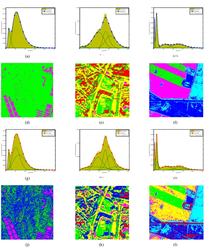
The EDSEM only separates water bodies and land roughly for the first three SAR images. The proposed HECM-FJ-GΓMM can distinguish more scattering components than the EDSEM, besides both correctly identifying two classes for the “India-Port” image. For example, Fig. 6(d) and (j) show the resulting classification maps for EDSEM and HECM-FJ-GΓMM, respectively. The land meta-class in Fig. 6(d) is further divided into three classes in Fig. 6(f): bare land, vegetation-cover land, and man-made building. Moreover, we illustrate the EDSEM and HECM-FJ-GΓMM estimated mixtures with the plots of components for the “Toulouse” and “Foulum” images, and their corresponding classification maps in the second and third columns of Fig. 6. The visual comparison validates the better class-discriminative capability of HECM-FJ-GΓMM. Specifically, as shown in Fig. 6(e), the under-segmentation occurs between the classes trees and buildings. By contrast, the Bayesian classification based on HECM-FJ-GΓMM PDF estimates gives more accurate and complete classification results, see five classes with different backscattering levels: shadow, road, land, tree, and building (respectively corresponding to the purple, yellow, green, blue, red colors in Fig. 6(k)). Similarly, it is interesting to see from Fig. 6(l) that the land class together with the vegetation class detected by EDSEM in Fig. 6(f) is split into two classes due to the wide range of intensities covered within this class (i.e., high variance). The visual interpretation suggests that two types of crops are identified: rye (purple)
0 50 100 150 200 250 0 0.002 0.004 0.006 0.008 0.01 0.012 0.014 0.016 greylevel n or m a li ze d h is tog ra m histogram EDSEM Components (a) 0 50 100 150 200 250 0 0.005 0.01 0.015 greylevel n or m a li ze d h is tog ra m histogram EDSEM Components (b) 0 50 100 150 200 250 0 0.005 0.01 0.015 0.02 0.025 0.03 0.035 0.04 greylevel n or m a li ze d h is tog ra m histogram EDSEM Components (c) (d) (e) (f) 0 50 100 150 200 250 0 0.002 0.004 0.006 0.008 0.01 0.012 0.014 0.016 greylevel n or m a li ze d h is tog ra m histogram GΓMM Components (g) 0 50 100 150 200 250 0 0.005 0.01 0.015 greylevel n or m a li ze d h is tog ra m histogram GΓMM Components (h) 0 50 100 150 200 250 0 0.005 0.01 0.015 0.02 0.025 0.03 0.035 0.04 greylevel n or m a li ze d h is tog ra m histogram GΓMM Components (i) (j) (k) (l)
Fig. 6. The estimated mixtures with the plots of components and their classification maps according to Bayesian decision rule: (Left to
Right) corresponding to the “Sanchagang-HH” TerraSAR-X image, “Toulouse” RAMSES image, and “Foulum” EMISAR image, respectively; (Top to Bottom) EDSEM estimate with the plots of components, EDSEM classification map, HECM-FJ-GΓMM estimate with the plots of components, and HECM-FJ-GΓMM classification map.
Fig. 7. 16-bit “Port-au-Prince” COSMO-SkyMed image (size: 512× 512). TABLE II
QUANTITATIVEMEASURESOBTAINED BYEDSEMANDHECM-FJ-GΓMMWITH THEOPTIMALNUMBER OFMIXTURECOMPONENTS
FORTWO16-BITAMPLITUDE ANDA 8-BITINTENSITYSAR IMAGES
EDSEM HECM-FJ-GΓMM Image M∗ Selected Models DKS DsKL M∗ DKS DsKL “India-Port16” 2 {f4, f1} 0.0056 0.0091 2 0.0018 0.0053 “Port-au-Prince16” 3 {f1, f8, f4} 0.0081 0.0289 5 0.0012 0.0169 “Ottawa” – – – – 4 0.0026 0.0081
with its lower intensity responses and wheat (yellow) with higher intensities, as well as low vegetation (blue) and high vegetation (red). We stress that the classification and modeling results obtained with the proposed method and EDSEM may differ appreciably for some landcover classes due to the different PDF families exploited in the mixture models. Certainly, further classes can be discriminated, if the polarimetric information is available [42].
C. Further Experimental Analysis
The SAR image data are quantized on a discrete scale, for example, 8 bits or 16 bits per pixel. A large-scale quantization yields the wide dynamic range of pixel values. To test the applicability of HECM-FJ-GΓMM, we conduct further experimental evaluation on two 16-bit SAR images: 1) the original 16-bit counterpart to the “India-Port” image shown in Fig. 2(a); and 2) a subscene (see Fig. 7) extracted from a 16-bit quantized StripMap COSMO-SkyMed amplitude image over Port-au-Prince (Haiti, HH polarization, geocoded ellipsoid corrected, 5m (ground range) × 5m (azimuth) resolution). For brevity, they will be denoted as “India-Port16” and “Port-au-Prince16”. The same parameter settings are employed as before except Mmax = 30 and ϵ = 1× 10⁻² for the “India-Port16”
image and Mmax = 40 and ϵ = 1× 10⁻² for the “Port-au-Prince16” image. In this test, a 2-component GΓMM
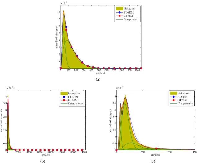
and a 5-component GΓMM are obtained, respectively, for the “India-Port16” and “Port-au-Prince16” images. Test results with corresponding measurements are shown in Fig. 8 and Table II. From these two examples, it can be seen that the estimated PDFs match well the observed heavy-tailed histograms, and the obtained quantitative results confirm the accuracy and effectiveness of the proposed method. In addition, we provide the obtained results with the EDSEM model (see Fig. 8 and Table II) for comparison, which correspondingly yields the PDF estimates with 2 and 3 components. The proposed HECM-FJ-GΓMM outperforms the EDSEM for both indexes.
We proceed by experimentally validating the robustness of the proposed estimator to the radiometric resolution. This is done by comparing the estimates obtained on the above initial 16 bit-per-pixel images and their compressed 8-bit versions. For 8-bit data of the “Port-au-Prince16” image, HECM-FJ-GΓMM also yields the 5-component GΓMM, whose plots are shown in Fig. 9. To perform the quantitative comparison, we stretch the PDF estimate
p(x|Θ) of GΓMM in 8 bits to the original dynamic range by scaling the argument (with a factor inverse to the
0 100 200 300 400 500 600 700 800 900 1000 0 1 2 3 4 5 6 7 8 x 10 greylevel n o rm a li ze d h is to g ra m histogram EDSEM GΓMM Components (a) 0 2000 4000 6000 8000 10000 12000 14000 0 0.5 1 1.5 2 2.5 3 3.5 4 x 10⁻³ greylevel n o rm a li ze d h is to g ra m histogram EDSEM GΓMM Components (b) 0 500 1000 1500 0 0.5 1 1.5 2 2.5 3 3.5 4 x 10⁻³ greylevel n o rm a li ze d h is to g ra m histogram EDSEM GΓMM Components (c)
Fig. 8. Histogram and the estimated PDFs of EDSEM and HECM-FJ-GΓMM with the plots of components: (a) “India-Port16” TerraSAR-X image, (b) “Port-au-Prince16” COSMO-SkyMed image, and (c) Zoomed-in result for (b).
on the initial 16-bit data results in DKS = 0.0020, DsKL = 0.0024 and DKS = 0.0136, DsKL = 0.0101,
respectively, for the “India-Port16” and “Port-au-Prince16” images. On the one hand, the difference obtained on “India-Port16” is almost negligible, which is consistent with the visual interpretation of Fig. 4(a) and Fig. 8(a). On the other hand, the relatively large DKS and DsKL are observed in the case of “Port-au-Prince16”. This is
due to the fact that most pixels cluster in a very narrow range of gray levels such that uniform scaling causes the histogram change from bimodality toward unimodality, see Fig. 9(a). Although the resulting histogram preserves the heavy tails of the initial 16-bit data, the pixels corresponding to the central part of histogram lose a great deal of details, which hinders the follow-up image processing and interpretation. In general, tail truncation is preferable to address this issue before scaling. From Fig. 9(b), we can observe that HECM-FJ-GΓMM is still effective, and the scaling histogram with truncating threshold3 equal to T = 5101 shows the visual bimodal behavior like that of original “Port-au-Prince16” image, exhibiting substantial differences from the uniformly-compressed histogram depicted in Fig. 9(a).
Next the performance of the developed model on the intensity image is investigated. Note that even though the performance of GΓD has been experimentally validated only on amplitude data [5], this model is a generalization of the Gamma distribution – a widely used tool for intensity SAR data modeling. As such, application of the designed HECM-FJ-GΓMM to intensity data is potentially of high interest. In contrast, the EDSEM has to update the underlying dictionary with available PDFs, otherwise the resulting estimates are of little physical interest. For this experiment, we employ another SAR image: a VV polarimetric CONVAIR-580 SAR intensity image over Ottawa (Canada, 8-bit quantized, a 10x azimuth multilooking), denoted as “Ottawa”. In initialization process, we still set equal weights πm = 1/Mmax, but let νm = 1 and κm = 1 for ∀ m ∈ [1, Mmax] (i.e., exponential case)
0 50 100 150 200 250 0 0.05 0.1 0.15 0.2 greylevel n o rm a li z e d h is to g ra m histogram GΓMM (a) 0 50 100 150 200 250 0 0.01 0.02 0.03 0.04 0.05 0.06 0.07 0.08 greylevel n o rm a li z e d h is to g ra m histogram GΓMM (b)
Fig. 9. Histogram and the estimated PDFs of HECM-FJ-GΓMM on the “Port-au-Prince16” COSMO-SkyMed image: (a) 8-bit
uniformly-compressed version, and (b) 8-bit uniformly-compressed statistics after truncation.
and uniformly choose Mmax data points from available gray levels of a given image as the mean of exponential
components to determine σm’s. Initial values for Mmax and ϵ are selected to be Mmax = 30 and ϵ = 1× 10⁻².
Fig. 10 shows the “Ottawa” image and its corresponding PDF estimate of HECM-FJ-GΓMM with the plots of components. It allows achieving the 0.0026 KS distance and the 0.0081 sKL divergence. As expected, the proposed method demonstrates good results in fitting the statistics of intensity SAR image.
Finally, we consider the “India-Port” image to analyze the effect of downsampling. In the following experiments, the downsampling in 2× 2 and 4 × 4 blocks by averaging is employed to create subsampled images. Note that since the pixel spacing is roughly half the value of the spatial resolution for this dataset, the original dataset is oversampled and the 2×2 averaging yields the data at its actual physical resolution. With the same initial conditions as presented in Section B (i.e., Mmax = 20, ϵ = 3× 10², and πm = 1/Mmax), the proposed HECM-FJ-GΓMM
algorithm has been applied to these two downsampled images. The resulting PDF estimates both are 2-component GΓMM, which, together with the corresponding normalized histograms, are illustrated in Fig. 11. The quantitative results are as follows: DKS = 0.0043, DsKL = 0.0074, and DKS = 0.0040, DsKL = 0.0131, after 2× 2 and
4× 4 downsampling, respectively. In both cases, HECM-FJ-GΓMM performs well in fitting the histograms of the
downsampled images. It is well known that downsampling is equivalent to spatial multilooking. Higher values of the equivalent number of looks (ENL) result in the lower the presence of speckle noise in the images. With the increase of ENL, two regions become more distinguishable such that the histogram exhibits obvious bimodal structure, which can be readily observed in Fig. 11. The “Toulouse” image is an example of high ENL in test dataset, for which we further do the experiment to compare with standard Gaussian mixture model (GMM). To this end, 5-component GMM (denoted as 5GMM) fitting estimate is presented in Fig. 12(a), reporting DKS = 0.0078
and DsKL = 0.0169 from the data. The quantitative comparison with the values in Table I for GΓMM suggests that
5GMM yields relatively worse result, and therefore less efficient for this dataset. In addition, from Fig. 12(a), we can see that a visually unsatisfactory accuracy of fit is presented by 5GMM. On the contrary, due to the flexibility of GΓD, GΓMM can improve the estimation performance, especially in the peak and the left-hand tail of histogram, see Fig. 12(b).
VI. CONCLUSION
This paper has explored the statistical analysis of high-resolution SAR images from the semi-parametric per-spective. To accomplish this goal, we have introduced a generalized Gamma mixture model (GΓMM) due to the good properties of the underlying GΓD, such as its very flexible and compact form. The identifiability of this kind of mixtures has been demonstrated to ensure that the statistical estimation problem is well-posed. Further, the unsupervised learning algorithm for GΓMM, namely HECM-FJ-GΓMM, has been developed by integrating the proposed histogram-based ECM algorithm into the Figueiredo-Jain algorithm, that allows us to simultaneously estimate the parameters of the model and determine the optimal number of mixture components at a relatively low computational cost. The experimental results, obtained from the considered wide range of space/airborne SAR
(a) 0 50 100 150 200 250 0 0.002 0.004 0.006 0.008 0.01 0.012 0.014 0.016 greylevel n o rm a li z e d h is to g ra m histogram GΓMM Components (b)
Fig. 10. (a) “Ottawa” CONVAIR-580 SAR image (size: 220× 220). (b) Histogram and the estimated PDF of HECM-FJ-GΓMM with the
plots of components. 0 50 100 150 200 250 0 0.005 0.01 0.015 0.02 0.025 0.03 0.035 0.04 greylevel n o rm a li z e d h is to g ra m histogram GΓMM Components (a) 0 50 100 150 200 250 0 0.005 0.01 0.015 0.02 0.025 0.03 0.035 0.04 0.045 0.05 greylevel n o rm a li z e d h is to g ra m histogram GΓMM Components (b)
Fig. 11. Histogram and the estimated PDF of HECM-FJ-GΓMM with the plots of components: (a) 2×2 downsampled image of “India-Port”,
and (b) 4× 4 downsampled image of “India-Port”.
0 50 100 150 200 250 0 0.005 0.01 0.015 greylevel n o rm a li z e d h is to g ra m histogram 5GMM Components (a) 0 50 100 150 200 250 0 0.005 0.01 0.015 greylevel n or m a li ze d h is tog ra m histogram GΓMM Components (b)
Fig. 12. Histogram and the estimated PDF of 5GMM and GΓMM with the plots of components for the “Toulouse” image: (a) 5GMM,
images with various scenes, prove the proposed GΓMM model and the designed estimator to be efficient and flexible in modeling the challenging bi/multimodal, heavy tailed SAR image data. Future work will be devoted to investigating the unsupervised contextual segmentation of high-resolution SAR images by combining HECM-FJ-GΓMM and spatial context within a Markov random field (MRF) framework.
ACKNOWLEDGMENT
The authors would like to thank European Space Agency (ESA) and Infoterra GmbH for providing the “Foulum”, “Ottawa”, and “India-Port”, “Sanchagang” SAR images, which are available at http://earth.esa.int/polsarpro/ and http://www.infoterra.de/, respectively, as well as Italian Space Agency (ASI) for providing the “Livorno” and “Port-au-Prince16” COSMO-SkyMed images. The experiments on the “Toulouse” RAMSES image, given by the French space agency (CNES), have been performed at INRIA by the second and fourth authors. The authors would also like to thank the Editor-in-Chief, the anonymous Associate Editor, and the reviewers for their insightful comments and suggestions, which have greatly improved the paper.
REFERENCES
[1] C. J. Oliver and S. Quegan, Understanding Synthetic Aperture Images. Norwood, MA: Artech House, 1998.
[2] H. C. Li, W. Hong, Y. R. Wu and P. Z. Fan, “An efficient and flexible statistical model based on generalized Gamma distribution for amplitude SAR images,” IEEE Trans. Geosci. Remote Sens., vol. 48, no. 6, pp. 2711-2722, Jun. 2010.
[3] R. O. Duta, P. E. Hart, and D. G. Stork, Pattern Classification, 2nd ed. New York, USA: John Wiley & Sons, 2001.
[4] C. Tison, J. M. Nicolas, F. Tupin, and H. Maitre, “New statistical model for Markovian classification of urban areas in high-resolution SAR images,” IEEE Trans. Geosci. Remote Sens., vol. 42, no. 10, pp. 2046-2057, Oct. 2004.
[5] H. C. Li, W. Hong, Y. R. Wu, and P. Z. Fan “On the empirical-statistical modeling of SAR images with generalized Gamma distribution,”
IEEE J. Sel. Topics Signal Process., vol. 5, no. 3, pp. 386-397, Jun. 2011.
[6] J. W. Goodman, “Statistical properties of laser speckle patterns,” in Laser Speckle and Related Phenomena. Heidelberg, Germany: Springer-Verlag, 1975, pp. 9-75.
[7] E. E. Kuruoglu and J. Zerubia, “Modeling SAR images with a generalization of the Rayleigh distribution,” IEEE Trans. Image Process., vol. 13, no. 4, pp. 527-533, Apr. 2004.
[8] G. Moser, J. Zerubia, and S. B. Serpico, “SAR amplitude probability density function estimation based on a generalized Gaussian model,” IEEE Trans. Image Process., vol. 15, no. 6, pp. 1429-1442, Jun. 2006.
[9] C. J. Oliver, “A model for non-Rayleigh scattering statistics,” Opt. Acta, vol. 31, no. 6, pp. 701-722, Jun. 1984.
[10] A. C. Frery, H. J. Muller, C. C. F. Yanasse, and S. J. S. Sant’Anna, “A model for extremely heterogeneous clutter,” IEEE Trans. Geosci.
Remote Sens., vol. 35, no. 3, pp. 648-659, May 1997.
[11] G. J. McLachlan and D. Peel, Finite Mixture Models. New York: Wiely, 2000.
[12] G. Moser, J. Zerubia, and S. B. Serpico, “Dictionary-based stochastic expectation-maximization for SAR amplitude probability density function estimation,” IEEE. Trans. Geosci. Remote Sens., vol. 44, no. 1, pp. 118-200, Jan. 2006.
[13] V. A. Krylov, G. Moser, S. B. Serpico, and J. Zerubia, “Enhanced dictionary-based SAR amplitude distribution estimation and its validation with very high-resolution data,” IEEE. Geosci. Remote Sens. Lett., vol. 8, no. 1, pp. 148-152, Jan. 2011.
[14] J. M. Nicolas, “Introduction to second kind statistic: application of log-moments and log-cumulants to SAR image law analysis,” Trait.
Signal, vol. 19, no. 3, pp. 139-167, Mar. 2002.
[15] G. Celeux and J. Diebolt, “The SEM algorithm: a probabilistic teacher algorithm derived from the EM algorithm for the mixture problem,” Comput. Stat. Quart., vol. 2, no. 1, pp. 73-82, Jan. 1985.
[16] M. A. T. Figueiredo and A. K. Jain, “Unsupervised learning of finite mixture models,” IEEE Trans. Pattern Anal. Mach. Intell., vol. 24, no. 3, pp. 381-396, Mar. 2002.
[17] E. W. Stacy, “A generalization of the Gamma distribution,” Ann. Math. Statist., vol. 33, no. 3, pp. 1187-1192, Mar. 1962. [18] H. Teicher, “Identifiability of finite mixtures,” Ann. Math. Statist., vol. 34, no. 4, pp. 1265-1269, Dec. 1963.
[19] N. Atienza, J. G. Heras, and J. M. M. Pichardo, “A new condition for identifiability of finite mixture distributions,” Metrika, vol. 63, no. 2, pp. 215-221, Apr. 2006.
[20] A. P. Dempster, N. M. Laird, and D. B. Rubin, “Maximum likelihood from incomplete data via EM algorithm,” J. Royal Statist. Soc.,
Ser. B, vol. 39, no. 1, pp. 1-38, 1977.
[21] J. Bilmes, “A gentle tutorial on the EM algorithm and its application to parameter estimation for Gaussian mixture and hidden Markov models,” University of Berkely, Tech. Rep. ICSI-TR-97-021, 1997.
[22] M. Abramowitz and L. A. Stegun, Handbook of Mathematical Functions. New York: Dover, 1972.
[23] X. L. Meng and D. Rubin, “Maximum likelihood estimation via the ECM algorithm: a general framework,” Biometrika, vol. 80, no. 2, pp. 267-278, 1993.
[24] X. L. Meng, “On the rate of convergence of the ECM algorithm,” Ann. Statist., vol. 22, no. 1, pp. 326-339, 1994.
[25] T. P. Minka, “Beyond Newton’s method,” [Online]. Available: http://research.mi-crosoft.com/ minka/papers/newton.html, 2000. [26] W. R. Press, S. A. Teukolsky, W. T. Wetterling, and B. P. Flannery, Numerical Recipes in C. London, U.K.: Cambridge Univ. Press,
2002.
[27] C. F. J. Wu, “On the convergence properties of the EM algorithm,” Ann. Statist., vol. 11, no. 1, pp. 95-103, 1983. [28] G. Schwarz, “Estimating the dimension of a model,” Ann. Statist., vol. 6, no. 2, pp. 461-464, 1978.