Factors influencing the precision and accuracy of Nd isotope measurements by thermal ionization mass spectrometry

HAL Id: hal-01720763

https://hal.uca.fr/hal-01720763

Submitted on 5 Mar 2018

HAL is a multi-disciplinary open access

archive for the deposit and dissemination of sci-entific research documents, whether they are pub-lished or not. The documents may come from teaching and research institutions in France or abroad, or from public or private research centers.

L’archive ouverte pluridisciplinaire HAL, est destinée au dépôt et à la diffusion de documents scientifiques de niveau recherche, publiés ou non, émanant des établissements d’enseignement et de recherche français ou étrangers, des laboratoires publics ou privés.

Factors influencing the precision and accuracy of Nd

isotope measurements by thermal ionization mass

spectrometry

Marion Garçon, Maud Boyet, Richard Carlson, Mary Horan, Delphine

Auclair, Timothy Mock

To cite this version:

Marion Garçon, Maud Boyet, Richard Carlson, Mary Horan, Delphine Auclair, et al.. Factors influenc-ing the precision and accuracy of Nd isotope measurements by thermal ionization mass spectrometry. Chemical Geology, Elsevier, 2018, 476, pp.493-514. �10.1016/j.chemgeo.2017.12.003�. �hal-01720763�

Factors influencing the precision and accuracy of Nd isotope

measurements by thermal ionization mass spectrometry

Marion Garçon

, Maud Boyet

, Richard W. Carlson

, Mary F. Horan

,

Delphine Auclair

, Timothy D. Mock

Published in Chemical Geology

1 _{ETH Zürich, Department of Earth Sciences, Institute of Geochemistry and Petrology,}

Clausiusstrasse 25, 8092 Zürich, Switzerland

2 _{Université Clermont Auvergne, CNRS, IRD, OPGC, Laboratoire Magmas et Volcans,}

F-63000 Clermont-Ferrand, France

3 _{Carnegie Institution for Science, Department of Terrestrial Magnetism, 5241 Broad Branch}

Road, NW, Washington DC 20015-1305, United States

* Corresponding author

E-mail: marion.garcon@erdw.ethz.ch Phone: +41 44 632 3745

Present address: ETH Zürich, Department of Earth Sciences, Institute of Geochemistry and Petrology, Clausiusstrasse 25, 8092 Zürich, Switzerland

To cite this paper:

Garçon M., Boyet M., Carlson R.W., Horan M. T., Auclair D., Mock T.D., Factors influencing the precision and accuracy of isotope measurements by thermal ionization mass spectrometry. Chemical Geology, 476, 493-514 (2018)

Abstract

Taking the example of Nd, we present a method based on a 4-mass-step acquisition scheme to measure all isotope ratios dynamically by thermal ionization mass spectrometry (TIMS); the aim being to minimize the dependency of all mass fractionation-corrected ratios on collector efficiencies and amplifier gains. The performance of the method was evaluated from unprocessed JNdi-1 Nd standards analyzed in multiple sessions on three different instruments over a period of ~ 1.5 years (n = 61), as well as from standards (18 JNdi-1 and 19 BHVO-2) processed through different chemical purification procedures. The Nd isotopic compositions of standards processed through fine-grained (25-50 µm) Ln-spec resin show a subtle but clear fractionation caused by the nuclear field shift effect. This effect contributes to the inaccuracy of Nd isotope measurements at the ppm level of precision.

Following a comprehensive evaluation of the mass spectrometer runs, we suggest several criteria to assess the quality of data acquired by TIMS, in particular to see whether the measurements were affected by domain mixing effects on the filaments. We define maximum tolerable Ce and Sm interference corrections and the minimum number of ratios to acquire to ensure the best possible accuracy and precision for all Nd isotope ratios. Changes in fractionation of Nd isotope ratios in between acquisition steps can result in significant inaccuracy and bias dynamic µ142 values by more than 15 ppm. To correct for these effects,

we developed a systematic drift-correction based on the monitoring of Nd isotope ratios through time. The residual components of scatter in the JNdi-1 and BHVO-2 datasets were further investigated in binary isotopic plots in which we modeled the theoretical effects of domain mixing on filaments, nuclear field shift and correlated errors from counting statistics using Monte-Carlo simulations. These plots indicate that the 4-step method returns precisions limited by counting errors only for drift-corrected dynamic Nd isotope ratios. Data acquired on three different TIMS instruments suggest the following composition for the JNdi-1 reference standard: 142Nd/144Nd = 1.141832 ± 0.000006 (2s), 143Nd/144Nd = 0.512099 ± 0.000005 (2s), 145Nd/144Nd = 0.348403 ± 0.000003 (2s), 148Nd/144Nd = 0.241581 ± 0.000003 (2s), and 150Nd/144Nd = 0.236452 ± 0.000006 (2s) when normalized to 146Nd/144Nd = 0.7219. Measurements performed on different instruments (TritonTM vs. Triton PlusTM) show resolvable differences of about 10 ppm for absolute 143Nd/144Nd, 145Nd/144Nd and 148Nd/144Nd ratios. The different criteria and corrections developed in this study could be applied to other isotopic systematics to improve and better evaluate the quality of high-precision data acquired by TIMS.

Keywords: Neodymium, TIMS, dynamic, static, isotopic composition 1. Introduction

Thermal ionization mass spectrometry (TIMS) is the state-of-the-art technique to measure isotope ratios at the ppm precision level provided that the element of interest has the right properties to ionize efficiently (see Carlson, 2014 for a review). The advent of multicollector TIMS allowed isotope ratios to be calculated by simultaneous collection of the ion beams of different masses, reducing the consequences of temporal variations in ion intensity and increasing the amount of signal integration per measurement interval, both of which foster higher precision isotope ratio determinations. The simplest of these methods is so-called static multicollection where all the ion beams are measured simultaneously. To calculate accurate isotope ratios from simultaneously detected ion beams requires knowledge of the amplifier gains and collection efficiencies of each faraday detector used in the measurement. The amplifier gains and faraday efficiencies theoretically can be eliminated through the technique of dynamic multicollection. In this approach, at least two magnet steps are made that move both the target and a standardizing isotope into the same faraday cup. The unknown isotope ratio is then calculated by combining the equations for the unknown ratio and the standardizing ratio in a way where the cup gains and efficiencies divide out. The relative deterioration of faraday collectors and their change of efficiency through time has been pinpointed as an important source of imprecision and inaccuracy for the determination of isotope ratios using static multicollection since the 1990’s (Makishima and Nakamura, 1991; Thirlwall, 1991). Similarly, changes in amplifier gain during measurement can affect isotope ratio determinations. The role of amplifier drift has been addressed by electronically rotating amplifiers between faraday cups so that any inaccuracy in the amplifier gains will be averaged over the entire measurement. By minimizing the consequences of relative cup inefficiencies and amplifier gain variability, the dynamic acquisition of isotope ratios avoids the consequences of cup deterioration and amplifier gain changes and yields better long-term precision and accuracy than static multicollection (Carlson, 2014; Fukai et al., 2017; Thirlwall, 1991).

Many studies have used the dynamic technique to investigate the small 142_{Nd anomalies}

created by the decay of 103 million year half-life 146_{Sm in both terrestrial and extra-terrestrial}

materials. Recent studies typically yield external isotope ratio precisions ranging from 3 to 8 ppm (2s) on the 142Nd/144Nd ratios of reference standards repeatedly measured through

different analytical sequences (cf. Bouvier and Boyet, 2016; Burkhardt et al., 2016; Carlson et al., 2007; O'Neil et al., 2008; Rizo et al., 2012; Roth et al., 2013). More recently, Burkhardt et al. (2016) and Fukai et al (2017) used a two mass-step acquisition method to calculate dynamic 148Nd/144Nd and 150Nd/144Nd ratios, in addition to 142Nd/144Nd ratios. Here, we propose a new method based on a 4 mass-step acquisition routine able to return all Nd isotope ratios dynamically, including the radiogenic 143Nd/144Nd ratio. We investigate the potential sources of imprecision and inaccuracy in the measurement of Nd isotope ratios by TIMS, and additionally suggest corrections to improve the quality of the data as well as criteria to recognize poor-quality runs after acquisition. While the study focuses on Nd, the processes, corrections and recommendations discussed here could potentially be applied to the measurement of other isotopic systems and provide keys to improve both the acquisition and the reduction of high-precision isotopic data in general.

2. The 4 mass-step method: principles and equations

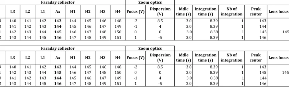
The dynamic measurement of all Nd isotope ratios involves the use of 4 different magnet settings per cycle. Two different mass-step sequences were tested to investigate how the mass fractionation rate affected the measurement of dynamic Nd isotope ratios (cf. Roth et al., 2014). They are shown in Table 1 together with run parameters such as voltages employed in the zoom optics, integration times, and the idle time spent before initiating signal integration after mass steps. The two tested configurations have the same collector positions, with the axial faraday cup successively centered on 143Nd, 144Nd, 145Nd, and 146Nd, and only differ by the order in which the acquisition lines are measured. Each 4-step cycle returns four static ratios for 142Nd/144Nd, 143Nd/144Nd, and 145Nd/144Nd, three static ratios for 148Nd/144Nd, one static ratio for 150Nd/144Nd, two dynamic ratios for 142Nd/144Nd, 143Nd/144Nd, and 148Nd/144Nd, three dynamic ratios for 145Nd/144Nd, and one dynamic 150Nd/144Nd ratio, all normalized to

146_Nd/144_{Nd = 0.7219.}

2.1. Equations for dynamic 142Nd/144Nd ratios

Dynamic ratios are calculated assuming that Nd mass fractionation follows an exponential law during the run (Andreasen and Sharma, 2009; Upadhyay et al., 2008). The veracity of this assumption for our measurements is re-examined below when evaluating the results in Section 4.1.1.a. The first dynamic 142Nd/144Nd ratio, !"#_!""!"_!"

the 142Nd/144Nd ratio measured on line 1, !"#_!""!"_!"

Meas 1, together with the

146_Nd/144_{Nd ratio}

measured on line 3, !"#_!""!"_!"

Meas 3, to minimize the difference of efficiencies and amplifier

gains between faraday collectors L1 and H1. This gives:

Nd !"# Nd !"" !"# ! = Nd !"# Nd !"" !"#$ ! × m!"# m!"" !! with F!= ln Nd !"# Nd !"" !"#$ Nd !"# Nd !"" !"#$ ! ln m!"# m_!"" (Eq. 1)

where m142, m144, and m146 are the atomic masses of isotopes 142Nd, 144Nd and 146Nd,

respectively; !"#_!""!"_!"

True= 0.7219 is the normalizing ratio used for mass fractionation

correction. Given that the measured ion-beam intensities depend on the collector efficiencies and amplifier gains, we can write:

Nd !"# Nd !"" !"#$ ! = 𝐼!"#Nd!"#$ ! 𝐼!""Nd !"#$ ! = 𝐼!"#Nd ! × 𝐶!! × 𝐺!! 𝐼!""Nd ! × 𝐶!! × 𝐺!! and !"#Nd Nd !"" !"#$ ! = 𝐼!"#Nd!"#$ ! 𝐼!""Nd !"#$ ! = 𝐼!"#Nd ! × 𝐶!! × 𝐺!! 𝐼!""Nd ! × 𝐶!! × 𝐺!! where 𝐼!"#Nd

!, 𝐼!""Nd!, 𝐼!"#Nd!, and 𝐼!""Nd! are the “ true ” intensities of the different Nd

isotope beams on acquisition lines 1 and 3; 𝐶!! and 𝐶!! are the efficiencies of the faraday

collectors L1 and H1 that change with time depending on instrument use; 𝐺!! and 𝐺!! are the

gains of the amplifiers to which the faraday collectors L1 and H1 are attached. Using this notation, (Eq.1) can be re-written as follows:

Nd !"# Nd !"" !"# ! = 𝐼!"#Nd! × 𝐶!! × 𝐺!! 𝐼!""Nd ! × 𝐶!! × 𝐺!! × exp ln Nd !"# Nd !"" !"#$ 𝐼!"#Nd ! × 𝐶!! × 𝐺!! 𝐼!""Nd ! × 𝐶!! × 𝐺!! ln m!"# m_!"" × ln m!"# m!"" ⟺ !"#Nd Nd !"" !"# ! = 𝐼!"#Nd! × 𝐶!! × 𝐺!! 𝐼!""Nd ! × 𝐶!! × 𝐺!! × Nd !"# Nd !"" !"#$ 𝐼!"#Nd ! × 𝐶!! × 𝐺!! 𝐼!""Nd ! × 𝐶!! × 𝐺!! ! with φ = ln m_!"# m_!"" ln m!"# m!"" ⟺ Nd !"# Nd !"" !"# ! =𝐼 Nd !"# ! 𝐼!""Nd ! × Nd !"# Nd !"" !"#$ ! × 𝐼 Nd !"# ! 𝐼!""Nd ! !! × 𝐶!! × 𝐺!! 𝐶!! × 𝐺!! !!! (Eq. 2)

Using m142 = 141.907729; m144 = 143.910093 and m146 = 145.913123 (AME2012, Wang et

al.(2012)), 𝜑 is equal to -1.013677, hence the faraday cup efficiencies and amplifier gains (i.e.

!!! × !!!

!!! × !!!) almost divide out completely in (Eq.2). This means that the calculation of dynamic

ratios mathematically reduces the non-ideal behavior of both the faraday collectors and the amplifier gains to a negligible contribution compared to the contribution they have on a static ratio. Indeed, following the same notation, the static !"#_!""!"_!" ratio from acquisition line 1 corresponds to: Nd !"# Nd !"" !"#"$% ! =𝐼!"#Nd! 𝐼!""Nd ! × Nd !"# Nd !"" !"#$ ! × 𝐼!"#Nd! 𝐼!""Nd ! !! ×𝐶!! × 𝐺!! 𝐶!! × 𝐺!! × 𝐶_!! × 𝐺_!! 𝐶!! × 𝐺!! !!

The relative difference between the static ratio from acquisition line 1 and the true value

!"

!"#

!"

!""

!"#$, that is the ideal case for which the faraday collector efficiencies C and the

amplifier gains G are all equal to 1, can be expressed in ppm as follows:

µ !"#" ! = !"#_!""Nd_Nd !"#"$% ! Nd !"# Nd !"" !"#$ − 1 × 10!₌ 𝐶!! 𝐶!!× 𝐶_!! 𝐶!! !! ×𝐺!! 𝐺!!× 𝐺_!! 𝐺!! !! − 1 × 10!

Similarly, the relative difference between the first dynamic ratio and the true value is:

µ !"# != !"#_!""Nd_Nd !"# ! Nd !"# Nd !"" !"#$ − 1 × 10!₌ 𝐶!! 𝐶!! !!! × 𝐺!! 𝐺!! !!! − 1 × 10!

Because 𝜑 ~ -1, one can see that µ !"# ! will always be close to zero while µ !"#" ! will scale to

~ !!!

!!! × !!!! ×

!!!

!!! × !!!!. One consequence of this result is that the precise calibration of the

amplifier gains is less critical when measuring dynamic ratios than it is for static ratios; nevertheless, we calibrate the gains every 24h to ensure the best possible accuracy and precision for our dynamic isotope measurements (see section 3.2.). Note also that the electronic rotation of the amplifiers at the end of a block that is available in the Triton software can help to decrease the contribution of 𝐺𝐿1

𝐺𝐻3 × 𝐺𝐻12 for the static ratio under the

conditions that each isotope is measured with every amplifier through the course of the run. Since the faraday collectors cannot be physically rotated, their efficiencies C, however, will always be an additional source of inaccuracy and imprecision in the acquisition of static and multistatic ratios compared to dynamic ratios.

As previously discussed by Roth et al. (2014), the fact that 𝜑 is not strictly equal to -1 implies that dynamic ratios also are not totally immune from collector inefficiencies and amplifier gains. The long-term accuracy of dynamic ratios should thus degrade slowly through time as collector performance deteriorates. Assuming that the amplifier gainsare properly calibrated and do not vary during a run (i.e. GH1 = GL1 = GH3 = 1), a simple sensitivity test shows that if

faraday collector L1 deteriorates faster than faraday collectors H1 and H3 so that !!!

!!! =

0.999900 and !!!

!!! = 1, then the static

!"

!"#

!"

!"" ratio will be shifted by µ !"#" ! = -100 ppm while

the dynamic !"#!""!"_!" ratio will only be biased by µ !"# ! = +1.4 ppm relative to the true value.

In percentage, this means that ~98.6% of the faraday collector effects are removed by the dynamic acquisition scheme.

Given the 4-line acquisition scheme, combining steps 2 and 4 provides another dynamic

142_Nd/144_{Nd ratio that removes ~98.6% of the relative cup efficiencies and amplifier gains of}

collectors L2 and Ax. This second dynamic ratio can be expressed as : Nd !"# Nd !"" !"# ! = Nd !"# Nd !"" !"#$ ! × Nd !"# Nd !"" !"#$ ! × Nd !"# Nd !"" !"#$ ! !! (Eq. 3) Or, in more detail:

Nd !"# Nd !"" !"# ! = 𝐼!"#Nd! 𝐼!""Nd ! × Nd !"# Nd !"" !"#$ ! × 𝐼!"#Nd! 𝐼!""Nd ! !! × C!" × G!" C!" × G!" !!!

The 4-line configuration thus allows the determination of two independent dynamic

142_Nd/144_{Nd ratios per cycle. Therefore, even if a 4-line cycle lasts twice as long as a 2-line}

cycle, the total signal acquisition time of a run is nearly the same as for the common 2-line method line to get a given number of dynamic ratios. For example, aiming to get 1000

142_Nd/144_{Nd dynamic ratios per run would require the acquisition of 1000 cycles with the}

common 2-line method and only 500 cycles with the 4-line method because each cycle produces two independent 142Nd/144Nd dynamic ratios.

2.2. Equations for dynamic 143Nd/144Nd ratios

Using the same principles as above, we combine ratios measured on steps 1-2-3 and 2-3-4 to calculate the two dynamic 143_Nd/144_{Nd ratios. The first dynamic} 143_Nd/144_{Nd ratio,}

!" !"#

!" !""

Dyn 1, is obtained by multiplying the

!" !"#

!" !""

Meas 1, by the one measured on line 2, !" !"#

!" !""

Meas 2, to cancel out the efficiency and

gain of the axial collector, and then by using the 146Nd/144Nd ratio measured on line 3,

!" !"#

!" !""

Meas 3, to correct for mass fractionation. This gives:

Nd !"# Nd !"" !"# ! = !"#Nd Nd !"" !"#$ ! × !"#Nd Nd !"" !"#$ ! × m!"# m_!"" !"! with F!= ln Nd !"# Nd !"" !"#$ Nd !"# Nd !"" !"#$ ! ln m!"# m_!"" that can be re-written as:

Nd !"# Nd !"" !"# ! = Nd !"# Nd !"" !"#$ ! ! ! × Nd !"# Nd !"" !"#$ ! ! ! × Nd !"# Nd !"" !"#$ ! × Nd !"# Nd !"" !"#$ ! !! (Eq. 4) = 𝐼 Nd !"# ! 𝐼!""Nd ! ! ! × 𝐼 Nd !"# ! 𝐼!""Nd ! ! ! × Nd !"# Nd !"" !"#$ ! × 𝐼 Nd !"# ! 𝐼!""Nd ! !! × C!" × G!" C!" × G!" ! !!! with γ = ln m!"# m_!"" ln m!"# m_!""

Using m143 = 142.909820; m144 = 143.910093 and m146 = 145.913123 (AME2012, Wang et

al.(2012)), γ = -0.504603. A variation of +100 ppm of the !!" × !!"

!!" × !!" ratio produces an increase

of ~ +0.5 ppm of the dynamic 143Nd/144Nd ratio, cancelling out ~99.5% of the relative cup efficiencies and gains between H1 and L1. The dynamic measurement of 143Nd/144Nd ratios is thus slightly more efficient in removing the relative cup gains and efficiencies than the dynamic 142_Nd/144_{Nd ratios.}

We derive a second dynamic 143Nd/144Nd ratio combining steps 2-3-4 to reduce relative efficiencies and gains between faraday cups L2 and Ax by ~99.5%:

Nd !"# Nd !"" !"# ! = !"#Nd Nd !"" !"#$ ! ! ! × !"#Nd Nd !"" !"#$ ! ! ! × !"#Nd Nd !"" !"#$ ! × !"#Nd Nd !"" !"#$ ! !! (Eq. 5) = 𝐼!"#Nd! 𝐼!!!Nd ! ! ! × 𝐼!"#Nd! 𝐼!""Nd ! ! ! × !"#Nd Nd !"" !"#$ ! × 𝐼!"#Nd! 𝐼!""Nd ! !! × C!" × G!" C_!" × G_!" ! !!!

The calculation of the three dynamic 145Nd/144Nd ratios is very similar to that of the dynamic

143_Nd/144_{Nd ratios. They result from the combination of ratios measured on lines 1-2, 2-3 and}

3-4 as shown below: Nd !"# Nd !"" !"# ! = !"#Nd Nd !"" !"#$ ! ! ! × !"#Nd Nd !"" !"#$ ! ! ! × !"#Nd Nd !"" !"#$ ! × !"#Nd Nd !"" !"#$ ! !! (Eq. 6) = 𝐼!"#Nd! 𝐼!""Nd ! ! ! × 𝐼!"#Nd! 𝐼!""Nd ! ! ! × !"#Nd Nd !"" !"#$ ! × 𝐼!"#Nd! 𝐼!""Nd ! !! × C!" × G!" C_!" × G_!" ! !!! Nd !"# Nd !"" !"# ! = Nd !"# Nd !"" !"#$ ! ! ! × Nd !"# Nd !"" !"#$ ! ! ! × Nd !"# Nd !"" !"#$ ! × Nd !"# Nd !"" !"#$ ! !! (Eq. 7) = 𝐼 Nd !"# ! 𝐼!""Nd ! ! ! × 𝐼 Nd !"# ! 𝐼!""Nd ! ! ! × Nd !"# Nd !"" !"#$ ! × 𝐼 Nd !"# ! 𝐼!""Nd ! !! × C!" × G!" C!" × G!" ! !!! Nd !"# Nd !"" !"# ! = Nd !"# Nd !"" !"#$ ! ! ! × Nd !"# Nd !"" !"#$ ! ! ! × Nd !"# Nd !"" !"#$ ! × Nd !"# Nd !"" !"#$ ! !! (Eq. 8) = 𝐼!"#Nd! 𝐼!""Nd ! ! ! × 𝐼!"#Nd! 𝐼!""Nd ! ! ! × !"#Nd Nd !"" !"#$ ! × 𝐼!"#Nd! 𝐼!""Nd ! !! × C!" × G!" C!" × G!" ! !!! with ϖ = ln m!"# m_!"" ln m!"# m_!""

Using m145 = 142.912579; m144 = 143.910093 and m146 = 145.913123 (AME2012, Wang et

al.(2012)), ω = 0.502213. Dynamic 145Nd/144Nd ratios are the most efficient in cancelling out the relative difference in cup efficiencies and gains, reducing it by ~99.8%. Therefore a variation of +100 ppm of the !!"

!!" ratio generates a decrease of ~ 0.2 ppm of the second

dynamic 145Nd/144Nd ratio.

2.4. Equations for dynamic 148Nd/144Nd ratios

The two dynamic 148_Nd/144_{Nd ratios are calculated in a slightly different way, using measured} 148_Nd/146_{Nd ratios as in Fukai et al.(2017). Combining ratios measured on lines 1 and 3 gives:}

Nd !"# Nd !"" !"# ! = !"#Nd Nd !"# !"#$ ! × !"#Nd Nd !"" !"#$ × m!"# m_!"# !!

with F! = ln Nd !"# Nd !"" !"#$ Nd !"# Nd !"" !"#$ ! ln m!"# m_!"" Hence, Nd !"# Nd !"" !"# ! = !"#Nd Nd !"# !"#$ ! × !"#Nd Nd !"" !"#$ !!! × !"#Nd Nd !"" !"#$ ! !! (Eq. 9) = 𝐼!"#Nd! 𝐼!"#Nd ! × Nd !"# Nd !"" !"#$ !!! × 𝐼!"#Nd! 𝐼!""Nd ! !! × C!" × G!" C!" × G!" !!! with θ = ln m!"# m!"# ln m_m!"# !""

Similarly, we can combine lines 2 and 4 to obtain a second dynamic ratio: Nd !"# Nd !"" !"# ! = Nd !"# Nd !"# !"#$ ! × Nd !"# Nd !"" !"#$ !!! × Nd !"# Nd !"" !"#$ ! !! (Eq. 10) = 𝐼!"#Nd! 𝐼!"#Nd ! × Nd !"# Nd !"" !"#$ !!! × 𝐼!"#Nd! 𝐼!""Nd ! !! × C!" × G!" C!" × G!" !!! θ = 0.986731 using m148 = 147.916899; m144 = 143.910093 and m146 = 145.913123

(AME2012, Wang et al.(2012)). This means that dynamic 148Nd/144Nd ratios reduce the relative difference in cup efficiencies and gains by ~98.7%.

2.5. Equations for dynamic 150_Nd/144_{Nd ratios}

The calculation of the dynamic 150Nd/144Nd ratio is less straightforward than other dynamic ratios as it involves the efficiencies and gains of three cups while the other dynamic ratios involved only two cups. This also means that the dynamic 150Nd/144Nd ratio will be more affected by cup aging and deterioration. Note that the way we calculate dynamic 150Nd/144Nd ratios is different from Fukai et al.(2017). The latter used ratios measured in four different cups and involved the measured 142Nd/144Nd ratio while our calculations rely on three cups only and do not use 142Nd. Only one dynamic 150Nd/144Nd ratio can be calculated with our cup configuration. Combining ratios from steps 1 and 3 gives:

Nd !"# Nd !"" !"# ! = !"#Nd Nd !"# !"#$ ! × !"#Nd Nd !"! !"#$ × m!"# m_!"# !!!

with F!′ = ln Nd !"# Nd !"" !"# ! Nd !"# Nd !"" !"#$ ! ln m_m!"# !"" Hence, Nd !"# Nd !"" !"# ! = Nd !"# Nd !"# !"#$ ! × Nd !"# Nd !"" !"#$ × Nd !"# Nd !"" !"# ! ! × Nd !"# Nd !"" !"#$ ! !! with χ = ln m!"# m!"# ln m_m!"# !""

Using (Eq. 9), this can be re-written as follows Nd !"# Nd !"" !"# ! = !"#Nd Nd !"# !"#$ ! × !"#Nd Nd !"" !"#$ !!!!!" × !"#Nd Nd !"" !"#$ ! !!" × !"#Nd Nd !"# !"#$ ! ! × !"#Nd Nd !"" !"#$ ! !! (Eq. 11) = 𝐼!"#Nd! 𝐼!"#Nd ! × Nd !"# Nd !"" !"#$ !!!!!" × 𝐼!"#Nd! 𝐼!""Nd ! !!" × 𝐼!"#Nd! 𝐼!"#Nd ! ! × 𝐼!"#Nd! 𝐼!""Nd ! !! × C!" × G!" C_!" × G_!" !!! × C!" × G!" C_!"× G_!" !!!" θ = 0.986731 and χ = 0.986693 using m148 = 147.916899; m144 = 143.910093; m150 =

149.920902 and m146 = 145.9131226 (AME2012, Wang et al.(2012)). Assuming that faraday

cups H4 and H3 degrade similarly relative to H1, this translates into a reduction of 53.7% of the total cup efficiencies and amplifier gains, which is much less efficient than other dynamic ratios but still better than static multicollection. If the ratio !!" × !!"

!!" × !!" degrades faster than

!!" × !!"

!!"× !!" , then the total reduction of efficiencies and gains is better, for example about

81.9% if !!" × !!"

!!" × !!" varies by 80 ppm and

!!" × !!"

!!"× !!" by only 20 ppm. 3. Methods

We evaluated the results of the 4-step method using more than 60 individual runs of the JNdi-1 Nd reference standard (Tanaka et al., 2000) analyzed in multiple sessions over a period of ~1.5 years on 3 different instruments. Additionally, we processed JNdi-1 Nd standards through chemistry following two different Nd separation procedures and analyzed the

reference basalt BHVO-2 to see whether the precision and accuracy calculated from unprocessed standards were applicable to samples.

3.1. Sample digestion and separation of Nd by ion chromatography

The Nd isotopic composition of reference basalt BHVO-2 was analyzed from 10 different dissolutions, all independently processed through column chemistry. We digested about 100 mg of rock powder per Savillex beaker in a mixture of 5 mL of 29N HF + 1 mL of 14N HNO3

on a hot plate at ~130°C for ~60h. After complete dissolution, and evaporation of the acids, the residues were treated two times with 5 mL of 14N HNO3 to eliminate fluorides. The

samples were then converted to chlorides by adding 3 mL of 6N HCl, twice, drying between applications. The light rare earth elements (LREEs) were separated from the matrix on primary columns (Biorad columns) filled with cation-exchange resin AG50W-X8 (200-400 mesh) by eluting the major elements in 2N HCl, then the LREEs in 6N HCl.

From there, two different separation procedures were used to isolate Nd from the other LREEs. They are shown schematically in Figure 1. The first method, the MLA method, consisted of eluting the LREE with 2-methylactic acid (2-MLA) on long and thin quartz columns (20 cm length x 0.2 cm inner diameter) filled with cation-exchange resin AG50W-X8 (200-400 mesh) in NH3+ form to separate Nd from other LREEs (see Boyet and Carlson,

2005 for further details). The thin geometry of the columns allows a better separation of Nd from other LREEs, but has the inconvenience of significantly slowing down the elution of the acid through the resin. We thus performed the separation under pressure using pure N2 to

accelerate the elution to about 0.05 mL per minute. For each batch of 2-MLA acid, the pH was carefully adjusted to 4.7 and the REE elution profile was recalibrated to ensure good yields and efficient separation of Nd from other LREEs. The MLA separation (Figure 1) was performed twice to ensure the best possible removal of Ce, which interferes with Nd on mass 142. Finally, the Nd cut was further purified on quartz columns (6 cm length x 0.4 cm inner diameter) filled with Ln-Spec resin (50-100 µm) using large volumes of 0.2 N HCl as eluent. This allowed the almost total removal of residual Sm, which interferes with Nd on masses 144, 148 and 150. Overall, the MLA method can be performed in about 4 days. It usually provides a good separation of Nd from other REEs for basaltic matrices and yields relatively low blanks, here < 55 pg of Nd (n = 2). The main inconveniences are (1) the setting-up and calibration of the 2-MLA acid for the 2nd _{step of the method, (2) the non-reproducibility of the}

Nd yields from one sample to another, ranging from 60 to 100% Nd recovery, and (3) the sporadic presence of residual Ce in the Nd cuts for non-basaltic samples.

The second separation procedure, the NaBrO3 method (Figure 1), uses the oxidation of Ce to

Ce4+ to separate it from the other trivalent LREEs. Details about this technique can be found in Tazoe et al. (2007) and Li et al. (2015). In brief, it involves dissolving the LREE cut from the primary column in a mixture of 10N HNO3 + 20 mM NaBrO3 to oxidize Ce(III) to

Ce(IV). The concentrated nitric solution containing trivalent LREEs, therefore Nd(III), was then eluted on Ln-Spec resin (50-100 µm) in small columns (1.2 cm length x 0.7 cm inner diameter) while Ce(IV) complexed with the HDEHP of the Ln-Spec resin and remained adsorbed on the resin. This step was performed twice to ensure the total elimination of Ce from the LREE cut. The Nd cut was then processed through a fine Ln-Spec resin (25-50 µm) in quartz columns (6 cm length x 0.4 cm inner diameter) using 0.2N to 0.25N HCl as eluents to recover Nd. We used the finest type of Ln-Spec resin to achieve a better separation of Nd from its neighboring REE, in particular from Pr that is almost not separated from Nd with a coarser resin. Finally, the Nd cut was purified on a small column (2 cm length x 0.8 cm inner diameter) filled with cation resin AG50W-X8 (200-400 mesh) using 2N HNO3 and 2.5N to

6N HCl to remove the residual traces of Ba and NaBrO3. Compared to the MLA method, this

technique offers the advantage of being easy to set up (no calibration for the 2nd step) and is slightly quicker (i.e. ~ 3.5 days). The method provides good Nd recoveries, generally between 80 and 100%, and a good separation of Nd from Ce and Sm in all types of samples. In this study the NaBrO3 method yielded slightly higher blanks than the MLA method, perhaps due

to the use of NaBrO3. We measured 125 pg of Nd in the total procedural blank (n=1) but

acknowledge that the higher Nd content of the blank could also be due to random contamination (cf. Garçon et al., 2017). The main inconvenience of the NaBrO3 method is its

inability to totally eliminate Pr from the final Nd cut. The use of the finest Ln-Spec resin allows the removal of ~80-90% of Pr which usually produces mean 141Pr/144Nd ratios < 0.2 during Nd measurements on TIMS. We tested the effects of Pr on Nd isotope analyses by doping a JNdi-1 Nd standard with different amounts of Pr. The results are shown in Appendix A and discussed in Section 4.1.1.d.

Following the chemistry, we systematically analyzed an aliquot of 5% of each processed standard by quadrupole ICP-MS to calculate Nd recoveries and make sure that no residual traces of sample matrix or NaBrO3 solution were present in the Nd fraction loaded on

3.2. Filament loading and TIMS measurements

Neodymium isotope ratios were measured using a double Re filament assembly to enhance the ionization of Nd as a positive metal ion (Nd+) in the TIMS source. All measurements were performed with the highest quality of Re ribbons (zone-refined Re) that were outgassed for 1 hour at 3.5A under high vacuum and exposed to ambient atmosphere for a few days before loading. Between 750 and 1000 ng of Nd diluted in 1 to 2 µL of 2N HCl was loaded at ~ 0.8 A on one of the two Re filaments, onto small spots, usually ~1 mm-wide, to minimize potential mixing effects during measurements (Upadhyay et al., 2008). A small amount (< 0.5 µL) of freshly prepared 1N H3PO4 was added to all samples/standards measured at

Clermont-Ferrand, France to help stabilize the emission of Nd during measurement. After loading, the filaments were turned to dull red glow for 1 second in air.

The Nd isotopic compositions reported in this study were measured on three different TIMS instruments: the Thermo Scientific™ Triton™ of the Department of Terrestrial Magnetism (DTM), Carnegie Institution for Science (Washington DC, USA), the Thermo Scientific™ Triton™ and Triton Plus™ of the Laboratoire Magmas et Volcans (LMV), Clermont Auvergne University (Clermont-Ferrand, France). The three instruments were equipped with 1011Ω amplifiers on each of the nine-faraday collectors. A typical analytical sequence (one or two barrels) consisted of measuring two JNdi-1 reference standards first to check the proper functioning of the instrument and then one JNdi-1 standard every two or three samples. The physical position of the faraday collectors and the zoom optic parameters were optimized, when necessary, at the beginning of each analytical sequence with the ion beams emitted by a mixed standard of Nd, Sm and Ce. TIMS measurements were started when the source pressure was below 8 x 10-8 mbar, which was usually reached after a night of pumping and the addition of liquid nitrogen to a cold finger directly above the filaments. For each run, the ionization filament current was increased to ~ 4200 mA at a rate of 250-300 mA/minute. At the same time, the evaporation filament current was increased to 1000 mA at a rate of 50 mA/minute. The filament currents were then increased slowly at rates < 50 mA/minute to typical values of 4200-4350 mA for the ionization filament and 1200-1700 mA for the evaporation filament until a stable 142_{Nd intensity of ~ 5-6V was reached. The measurements}

were started after several automatic lens focuses involving all focus plates (Condenser, Left- and Right-Symmetry, X-, Y- and Z-Focus) to ensure the best possible extraction of Nd+ from

the filament to the exit slit of the ion source. Runs consisted of a maximum of 18 blocks of 30 cycles (i.e. 540 cycles, ~8 h) with baselines measured for 60 seconds in between each block.

To avoid large and imprecise mass fractionation corrections, measurements were stopped before the end of the 540 cycles when the 146Nd/144Nd ratio used to correct mass fractionation reached a value of 0.724 or when the 145Nd signal dropped below 0.5V in the axial cup. Each 5 blocks, peaks were centered in the axial cup for each magnet setting and the lenses were automatically refocused using 145Nd in the axial cup (i.e main magnet setting, line 3, Table 1). Calibration of the amplifier gains was performed every 24h. Rotation of the amplifiers between different faraday cups was not employed. To avoid abrupt changes of the filament temperature, the automatic heating routine provided with the Triton™ software was not used. When necessary, the evaporation filament current was increased at a very slow rate of 0.5 to 1 mA/minute during the data acquisition to maintain the stability of the Nd signal during measurement.

3.3. Data processing

Gain, baseline and isobaric interferences from 144, 148, 150_{Sm and} 142_{Ce were corrected online}

with the Triton™ software. From the corrected Nd intensities, all static and dynamic ratios were calculated offline using a Matlab routine available on request to the corresponding author. For each run, the routine selects only cycles for which the mean of the 146Nd/144Nd ratios acquired on lines 1-2-3-4 is lower than 0.724, and for which the 145Nd signal in the axial cup (acquisition line 3) is higher than 0.5 V. For each cycle, the static Nd ratios of each acquisition line are calculated by correcting mass fractionation with the exponential law and a

146_Nd/144_{Nd ratio of 0.7219. The dynamic Nd ratios are calculated following the equations}

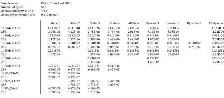
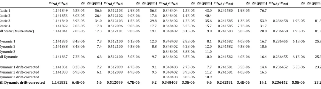
given in Section 2. The static and dynamic ratios of a run are calculated by averaging the ratios determined at each cycle and by screening for outliers at ± 2s, where s is the standard deviation of the run. The routine generates a table summarizing the mean static and dynamic Nd ratios together with the mean 146Nd/144Nd, 140Ce/144Nd, 147Sm/144Nd and 141Pr/144Nd ratios and their 2 s.e., where s.e. is the standard error of the mean (see Table 2 for an example). In Table 2, the means and standard errors of all static ratios (column “All static”) and all dynamic ratios (column “All dynamic”) are calculated by pooling the ratios obtained for each cycle all together, regardless of the acquisition lines from which they are derived; for example, if 540 cycles were acquired, the mean and error of all 142Nd/144Nd static ratios were calculated from 2160 ratios (4 static ratios per cycle) while the mean and error of all

142_Nd/144_{Nd dynamic ratios were calculated from 1080 ratios (2 dynamic ratios per cycle). In}

of the run and decide whether a measurement should be accepted or rejected. The different tests and criteria used to accept or reject a run are explained and discussed below in Section 4.1.1.

4. Results and discussion

4.1. The 4-step method: Precision and accuracy of Nd isotope measurements

4.1.1. Criteria to decide whether a run is acceptable

Based on previous work (Andreasen and Sharma, 2009; Sharma and Chen, 2004; Sharma et al., 1996; Roth et al., 2014; Upadhyay et al., 2008; Wielandt and Bizzarro, 2011) and new considerations, we suggest four criteria to help the analyst decide whether a run should be accepted or rejected, in particular when it shows unusual behavior such as reverse fractionation (i.e. when 146_Nd/144_{Nd ratios decrease through time). In the following evaluation}

of the results, we systematically rejected the runs that did not satisfy one or more of the four requirements listed below. The total rejection rate is estimated at about 10-15% for the present study. For example, 8 out of 61 runs were rejected for the JNdi-1 reference standards analyzed over ~1.5 years.

4.1.1.a. Mass fractionation following the exponential law

Previous studies have shown that the exponential law is the most accurate law to correct for mass fractionation occurring during Nd isotope measurements by TIMS (Andreasen and Sharma, 2009; Upadhyay et al., 2008). Our measurements of the JNdi-1 reference standard confirm that this is generally the case for the runs showing normal fractionation i.e.

146_Nd/144_{Nd ratios increasing through the analysis as expected if Nd+ is emitted from a single,}

homogenous domain on the filament. Figure 2a provides an example of such a behavior where the measured 142Nd/144Nd and 146Nd/144Nd ratios oscillate around the trend expected for a mass-bias that follows the exponential law (red line in Figure 2a). Runs may have short periods of time during which mass fractionation slightly departs from the exponential law and follows either the Rayleigh or the Power law. Since these periods of time are sporadic and usually very short compared to the total length of a run, there is, in our opinion, no obvious reason to correct the mass-bias by a law other than the exponential law. In addition, dynamic ratios corrected with the power law do not provide a more precise result compared to those corrected with exponential law.

In some runs, however, the relationship between measured 142Nd/144Nd and 146Nd/144Nd ratios shows large variations inconsistent with the trends predicted by any of the common

fractionation laws for very long periods of time, i.e. for several measurement blocks. This usually happens when the fractionation is reverse for a significant part of the run (i.e.

146_Nd/144_{Nd ratios decrease through the analysis) or switches from normal to reverse several}

times during the run. An example of the latter case is shown in Figures 2b-d. Reverse fractionation very likely indicates evaporation and mixing of Nd from variably fractionated domains on the filament (Andreasen and Sharma, 2009; Hart and Zindler, 1989; Russell et al., 1978; Sharma and Chen, 2004; Upadhyay et al., 2008). The mass fractionation of the Nd+ beam emitted by each domain individually follows the exponential law, but the Nd+ beam coming from the different domains that is finally extracted from the source and collected in the faraday cups follows linear mixing trends between the different domains. The amplitude of this effect cannot be predicted, and thus corrected, since it depends, at any given time, on the number of domains emitting Nd+, and on the amount and fractionation stage of Nd+ emitted by each domain. Although we loaded the samples/standards onto very small spots to minimize the formation of clumps, domain mixing on the filament is likely the reason why some runs exhibit large departures from common fractionation laws as shown in Figure 2b. Upadhyay et al.(2008) and Andreasen and Sharma (2009) demonstrated that using the exponential law to correct for mass fractionation when Nd is emitted from multiple domains can significantly bias 142Nd/144Nd, 148Nd/144Nd, and 150Nd/144Nd ratios towards higher than true values and 145Nd/144Nd towards lower values. Importantly, Andreasen and Sharma (2009) showed that data collected during, after, or before reverse fractionation are all affected by domain mixing effects. Therefore, to ensure the best possible measurement precision and accuracy, we rejected runs showing large and sporadic departures from the common fractionation laws, which was the case for 3 out of 61 runs in the present study. As shown in Figure 2b and d, this first criterion generally removes runs that show long or repetitive periods of reverse fractionation.

4.1.1.b. Poisson noise and minimum number of ratios to measure

Different sources of error can affect the measurement of dynamic Nd isotope ratios. Systematic errors, such as those induced by domain mixing on the filament, are difficult to predict and thus to correct. Random errors due to counting statistics (i.e. Poisson noise) or instrument electronic stability (mainly Johnson-Nyquist noise) are easier to predict, and their level can generally be minimized by optimizing measurement conditions. Figure 3a shows how the standard deviation of the combined dynamic 142Nd/144Nd ratios varies as a function of the mean 142Nd beam intensity of the runs. The strong relationship observed between

standard deviation and ion beam intensity, independent of the instrument and the analytical sequence, suggests that the main factor limiting the internal precision is ion counting statistics (i.e Poisson noise). To verify this hypothesis, we calculated the predicted Poisson noise 𝜎_! 𝑈_!"# for different 142Nd beam intensities as follows:

𝜎! 𝑈!"# =

𝑒 × 𝑅 × 𝑈_!"#

𝑡_! (Eq. 12)

where e is the elementary charge in Joules, R the feedback resistor in Ohms (in our case, R= 1011 Ω), U142 is the mean 142Nd beam of the run in Volts, ts is the integration time in seconds

(here ts = 8.389s x 2 since we calculate 2 independent dynamic 142Nd/144Nd ratios per cycle).

Using 142Nd/144Nd = 1.141835, and 146Nd/144Nd = 0.7219 as an average composition for the JNdi-1 standard, we estimate the Poisson noise on 144Nd and 146Nd intensities, propagate the errors on the measured 142_Nd/144_{Nd and} 146_Nd/144_{Nd ratios, and then on the dynamic} 142_Nd/144_{Nd ratios using Monte-Carlo simulations. The result of this calculation, shown by a}

dashed line in Figure 3a, well fits the observed trend between 142_{Nd beam intensity and}

standard deviation (1s). The slight shift of the data to the right of the modeled curve corresponds to an unknown additional imprecision of 0.1 to 0.2 ppm on the final standard error of the runs, which can be considered negligible. This confirms that counting statistics are the main factor limiting the internal precision of the measurements. Note that the contribution of amplifier noise level (i.e. Johnson-Nyquist noise) for the 1011 Ω feedback resistor to isotope ratio precision is negligible compared to the Poisson noise. The amplifier noise level ranges from a maximum of 3% of the Poisson noise at 1V to about 0.5% at 12V, as previously discussed by Wielandt and Bizzarro (2011).

Since the standard deviation of a run is predictable and controlled by beam intensity, one can define the minimum integration time (or minimum number of ratios) needed so that the mean of the dynamic 142Nd/144Nd ratios be determined at ± δ ppm with a 95% confidence level at any given intensity. Assuming that the distribution of 142Nd/144Nd ratios is normal, this involves calculation of the minimum number of ratios, N, needed to obtain a standard error

! !

≤

!

!_! , where 𝑧! is the critical value of the standard normal distribution corresponding to

the desired level of confidence c (𝑧! = 1.96 for a 95% confidence level), 𝜎 is the standard

deviation of the dynamic 142Nd/144Nd ratios (i.e. !"#_!""!"_!"

!"# !and !" !"# !" !"" !"# ! pooled

N ≥ 𝑧_𝛿! !× 𝑠! _{(Eq. 13)}

Knowing the relationship between standard deviation and 142Nd beam intensity (cf. Figure 3a), defines the minimum number of ratios to measure to establish a mean dynamic

142_Nd/144_{Nd ratio at ± 3, and ± 5 ppm with a 95% confidence level as a function of the mean} 142_{Nd intensity of a run (cf. Figure 3b). If the mean} 142_{Nd beam intensity of a run is 3V, one}

should measure at least 390 ratios to ensure the detection of a 5 ppm 142_{Nd anomaly with 95%}

confidence, and at least 1080 ratios if the aim is to detect a 3 ppm anomaly with 95% confidence. In the following evaluation of the results, we systematically rejected runs for which the number of measured ratios was too low to detect a 5-ppm anomaly with 95% confidence. This criterion led to the rejection of 3 out of 61 runs for the unprocessed JNdi-1 standards.

4.1.1.c. Stable cumulative mean for dynamic Nd isotope ratios

Measuring a large number of ratios is important to establish a mean value with a low internal error at a high confidence level. For this statement to be valid, however, requires that the mean of the measured ratios converges to the true value of the sample/standard by the end of the run. This implies that the cumulative mean of the measured ratios should reach a plateau before the end of the run when plotted against measurement cycle. In the run illustrated in figure 4a, the dynamic 142Nd/144Nd ratios converge to the mean value of the run within ± 1.5 ppm (2 s.e.) after only 120 cycles and stay within that error limit for the remainder of the run. While most runs exhibit a similar behavior, some runs never converged to a plateau, as shown in Figure 4b. This is problematic because in such a run, the final calculated mean value depends on the number of measured cycles. In Figure 4b, if the run was stopped after about 300 cycles, the final calculated dynamic 142_Nd/144_{Nd ratio is about 5 ppm lower than the value}

obtained after 540 cycles, a bias that is well above the final internal error reported for the run i.e. ± 1.5 ppm (2 s.e.). This behavior may again be related to domain mixing effects as the formation of variably fractionated domains on the filament after ~ 300 cycles would be compatible with the sudden increase of the mean dynamic 142Nd/144Nd value. This is also supported by the evolution of 146Nd/144Nd ratios through time, changing from a smooth increasing trend to a stable evolution after ~ 300 cycles (cf. Figure 4d). In the following, we developed a criterion that allows the identification of ‘unstable mean values’. We arbitrarily defined an unstable mean as a mean value that varies beyond ± 2 times the final standard error for the last quarter of the run. Runs yielding an unstable mean for the combined dynamic

142_Nd/144_{Nd ratios (2 runs out of 61 for the unprocessed JNdi-1 Nd standards) were rejected}

and not taken into account in the evaluation of the method results. The ‘unstable mean criterion’ can be more generally applied to all dynamic ratios.

4.1.1.d. Maximum isobaric interferences

Cerium and Sm are the most critical potential interfering elements as they both have isobars with Nd. Cerium interferes on mass 142, and hence affects the measurement of 142Nd/144Nd ratios, while Sm interferes on masses 144, 148, and 150, and hence impacts all Nd isotope ratios through its contribution to the normalizing isotope 144Nd. When residual Sm and/or Ce are present in the samples, isobaric interferences are generally corrected online using the measured 147_{Sm and} 140_{Ce beams and assuming constant values for the} 142_Ce/140_Ce, 144_Sm/147_Sm, 148_Sm/147_{Sm, and} 150_Sm/147_{Sm ratios. In this correction, the most important}

source of error arises from the fact that mass fractionation of the interfering element is not known, hence not taken into account for Ce and Sm isotope ratios. Since each element has its own fractionation trend through time on TIMS, using the fractionation factor of Nd to correct the Sm and Ce ratios, as commonly done on MC-ICP-MS, may introduce additional errors instead of improving the isobaric correction. To evaluate the effects of such an approximation, we propagated the errors arising from imprecise isobaric interference corrections on all Nd isotope ratios using Monte-Carlo simulations (Figure 5). The calculations were performed for different amounts of interfering Ce and Sm assuming that their isotope ratios were highly fractionated during measurement, that is with fractionation factors, f, varying between -1 and +1. This roughly corresponds to a 140Ce/142Ce ratio ranging from 0.123 to 0.128 and a 144Sm/147Sm ratio from 0.201 and 0.209 using atomic masses of Wang et al. (2012), and 140Ce/142Ce = 0.12565 and 144Sm/147Sm = 0.20506 as ‘true’ values (Chang et al., 1995; 2002). This extreme mass fractionation scenario allowed us to calculate the maximum amounts of Ce and Sm that can be tolerated in a sample to ensure that the errors induced by imprecise isobaric interference corrections remain lower than 5 ppm on all dynamic Nd isotope ratios. Our results indicate that ignoring the mass fractionation of the

140_Ce/142_{Ce ratio can lead to errors > 5 ppm on dynamic} 142_Nd/144_{Nd ratios as soon as the} 140_Ce/146_{Nd ratio is higher than ~ 1.6 x 10}-3 _{(Figure 5a). For Sm interference corrections, the}

situation is slightly more complex since the errors propagate to all Nd isotope ratios, but to different degrees. According to the simulations, the dynamic 150_Nd/144_{Nd ratio is the most}

affected by imprecise Sm isobaric interference corrections (Figure 5b). Errors on the determination of this ratio become higher than 5 ppm when the 147Sm/146Nd ratio of the

sample reaches a value of ~ 1.2 x 10-4. Note that the tolerance is higher for the dynamic

142_Nd/144_{Nd ratio since the propagated errors remain < 5 ppm as long as the} 147_Sm/146_{Nd ratio}

is below ~ 4.3 x 10-4. Therefore, unless the collector configuration allows for the determination of the precise fractionation stage of Ce and Sm during Nd analyses, we recommend that runs having mean 140Ce/146Nd and 147Sm/146Nd ratios > 1.6 x 10-3 and > 1.2 x 10-4, respectively, be systematically rejected. In this study, the maximum mean 140Ce/146Nd and 147Sm/146Nd ratios ever measured for a run were well below these limits i.e. 9.8 x 10-5 and 4.8 x 10-6, respectively (cf. Appendix A, B, C). Interferences of this magnitude also introduce the concern that such small signals are not easily quantified with faraday detectors equipped with 1011 _{Ohm resistors. For example, for a} 142_{Nd signal of 2V, a} 147_Sm/146_{Nd ratio of 5 x 10}-6

corresponds to a 147_{Sm signal of only 6 µV, which is indistinguishable from the noise in a}

faraday cup using amplifiers with a 1011 Ohm feedback resistor. Quantifying interferences at this scale thus requires either higher ohmage feedback resistors for the faraday cup amplifier used to detect the interference, or the use of ion multipliers, with the inherent difficulty of gain calibration between the detectors.

Another potential problem that may lead to imprecision in the determination of dynamic Nd isotope ratios is the presence of Pr. Praseodymium concentrations are 3-5 times lower than Nd concentrations in natural samples but the NaBrO3 method fails to effectively remove this

element from the Nd fraction (cf. Section 3.1). The most likely potential isobaric interference during Nd analysis by TIMS is by 141PrH on 142Nd. However, large Pr ion beams could also produce a peak tailing effect on 142Nd and thus bias 142Nd/144Nd ratios. To test whether these effects were important, we doped 3 JNdi-1 Nd standards with variable amounts of Pr to obtain solution that produced mean 141Pr/146Nd ratios from ~ 0.3 to 1.3. Results are shown in Appendix A together with un-doped JNdi-1 Nd standards. No systematic bias was observed on dynamic Nd isotope ratios as a function of Pr amounts; hence we conclude that the residual presence of Pr in samples is not problematic for the determination of precise Nd isotope ratios by TIMS, at least for samples with 141Pr/146Nd ratios < ~1.3.

4.1.2. Fractionation rate and drift correction

Dynamic measurements theoretically reduce most of the imprecision arising from collector inefficiencies and amplifier gains. The drawback, however, is that the ratios used for dynamic calculations are not measured at the same time, and hence can potentially record different stages of fractionation. Roth et al. (2014) suggested that, if Nd fractionates quickly, the lapse of time between the acquisition of the 146_Nd/144_{Nd and the} 142_Nd/144_{Nd ratios could be enough}

to induce large biases, up to 8 ppm, on dynamic 142Nd/144Nd ratios. The bias can be either positive or negative depending on the order in which the ratios used for dynamic calculations are acquired. For example, measuring the 146Nd/144Nd ratio before the 142Nd/144Nd, as done by Roth et al. (2014) and Upadhyay et al. (2009), may bias the dynamic 142Nd/144Nd ratios towards lower than true values for high fractionation rate. Conversely, measuring the

142_Nd/144_{Nd ratio first, as in our collector configuration (Table 1) may bias dynamic} 142_Nd/144_{Nd ratios towards higher than true values. The longer is the time gap and the higher}

is the fractionation rate, the larger will be the effect on dynamic Nd isotope ratios. In their study, Roth et al. (2014) calculated a threshold limit for the average fractionation rate of a run over which they estimated that the bias on dynamic 142_Nd/144_{Nd ratios should be higher than 5}

ppm. They suggested that any run having an average fractionation rate higher than the threshold limit should be treated as suspicious.

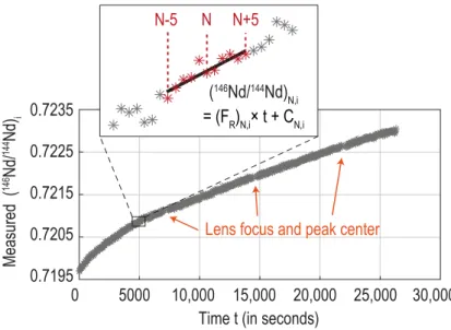
Here, we go further and suggest a method to systematically correct for the drift of Nd isotope ratios in between acquisition lines whatever the fractionation rate. The method consists of determining the local fractionation trend of Nd isotope ratios by fitting a least-square regression line through several consecutive measurements of the same ratio. Using the equation of the fitted line, the isotope ratios of interest can then be recalculated at any time t. An illustration of the method is shown in Figure 6 for the 146Nd/144Nd ratio acquired on line 3. This ratio is used, together with the 142Nd/144Nd ratio from acquisition line 1, to calculate the first dynamic 142Nd/144Nd ratio (cf. Eq. 2). To correct for the drift of 146Nd/144Nd ratios between lines 1 and 3, we approximated, for each cycle N, the local fractionation trend of

146_Nd/144_{Nd ratios as linear over 11 consecutive cycles, from N-5 to N+5 (see inset of Figure}

6). The number of cycles used to interpolate the fractionation trend should be large enough to minimize noise contribution, but small enough so that the local variation of 146Nd/144Nd ratios through time can always be approximated as linear. We found that 11 consecutive measurements was the best compromise to describe the variation of all Nd isotope ratios through time, regardless of the fractionation rate and the signal/noise ratio. Note that determining the equations of the local fractionation trends as a function of time t (and not as a function of cycles N) allows to properly take into account fractionation during blanking time, lens refocusing and peak centering when no measurement is performed. The drift-correction assumes a linear fractionation over 11 consecutive measurements, and hence requires that the evolution of Nd isotope ratios be as smooth as possible. Abrupt changes or step-variations such as those caused by the automatic heating function of the Triton™ software at the end of

each block, or accompanying changes in source focus, likely will make the correction imprecise.

Assuming that the data were collected with collector configuration 1 (Table 1), we used the equation of the fitted fractionation line to recalculate the value of the 146Nd/144Nd ratio as if it was measured two lines before (i.e. 2x8.39 seconds (integration time) + 2x3 seconds (idle time) = 22.78 seconds earlier), at the time when the 142Nd/144Nd ratio was acquired. This drift-corrected 146Nd/144Nd ratio was then used to calculate the drift-corrected dynamic 142Nd/144Nd ratio following Eq. (2). The same correction is applied to the second dynamic 142Nd/144Nd ratio and to the dynamic 148Nd/144Nd ratios by monitoring the fractionation trends of

146_Nd/144_{Nd ratios measured on different acquisition lines and by recalculating their values at}

the desired time. Correcting the dynamic 143_Nd/144_Nd, 145_Nd/144_{Nd, and} 150_Nd/144_{Nd ratios for}

drift is a bit trickier as they use more than two measured ratios, sometimes from three different acquisition lines (cf. Eq. 4-5, Eq. 6-8 and Eq. 11). Hence, one needs to interpolate the variations of 143Nd/144Nd, 145Nd/144Nd and 148Nd/144Nd through time, in addition to those of 146Nd/144Nd, and recalculate their values at the same time t. In the following, drift-corrected

143_Nd/144_Nd

Dyn 1 and 145Nd/144NdDyn 1 were determined with ratios brought back to the

acquisition time of line 2, drift-corrected 143Nd/144NdDyn 2, 145Nd/144NdDyn 2, and 150_Nd/144_Nd

Dyn 1 with ratios recalculated at the acquisition time of line 3, and drift-corrected 145_Nd/144_Nd

Dyn 3 with ratios recalculated to the acquisition time of line 4. The effects of the

drift-correction on all dynamic Nd isotope ratios are discussed in the following section of the manuscript.

4.1.3. Comparison of the different ratios acquired during a run 4.1.3.a. Static vs. dynamic Nd isotope ratios

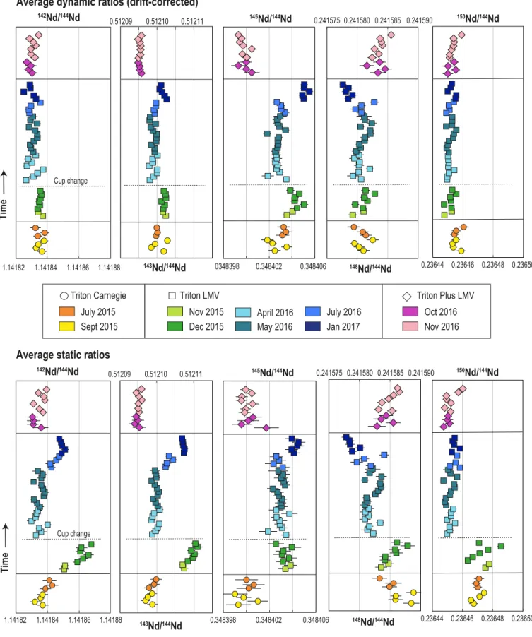
Figure 7 compares static and dynamic Nd isotope ratios of JNdi-1 Nd standards acquired over a period of ~1.5 years on the Triton™ from Carnegie, and the Triton™ and Triton Plus™ from LMV. The measured ratios and a compilation of the means and standard deviations are provided in Appendix A and Table 3, respectively. The data confirm that, over long periods of time, dynamic Nd isotope measurements yield better long-term reproducibility and more accurate results than static measurements due to the removal of the component of scatter arising from collector inefficiencies and amplifier gains (cf. Section 2). Average static ratios have external precisions ~1.5 to 3 times worse than dynamic ratios, except for 145Nd/144Nd ratios (Table 3). The latter exhibit large variations on individual static ratios but a surprisingly good external precision on the average of all static ratios that can be mathematically explained

by the fortunate cancellation of several cup efficiencies and amplifier gains when averaging the four static 145Nd/144Nd ratios. As previously noticed by several authors (Carlson, 2014; Fukai et al., 2017; O'Neil et al., 2008), the change of the whole set of faraday cups, including the axial cup, in the LMV Triton™ (green and blue squares in Figure 7) resulted in a large shift, up to 100 ppm, of the static ratios. Following this shift, the set of collectors of the LMV Triton™ may have slowly deteriorated and caused the static ratios to deviate between April 2016 and January 2017 (cf. blue squares in Figure 7). The imprecision and inaccuracy of static ratios over long periods of time can also be highlighted on binary plots, as illustrated in Figure 8 where static 142_Nd/144_{Nd ratios from acquisition line 1 (i.e.} 142_Nd/144_Nd

Static 1) are

reported as a function 148_Nd/144_Nd

Static 3. Equations for exponential mass-fractionation

correction show that the 142_Nd/144_Nd

Static 1 and 148Nd/144NdStatic 3 scale to roughly the same

combination of collector efficiencies and amplifier gains, that is to ~ CL1 × GL1

CH12 × GH12 × CH3× GH3.

In Figure 8, the deterioration of these faraday cups translate into the strong positive co-variation of 142Nd/144NdStatic 1 and 148Nd/144NdStatic 3 measured in JNdi-1 Nd standards on the

LMV Triton™. Deviations of static ratios due to cup deterioration are observed at the scale of one analytical session i.e. within two weeks of measurements when cups are relatively old (cf. green squares in Figure 8), which reinforces the need to determine all Nd isotope ratios dynamically to ensure the best possible accuracy. The number of data acquired on the Carnegie Triton™ might not be enough to precisely determine the trend resulting from cup deterioration, but it seems that the instrument use may have caused the static ratios to deviate in the opposite way compared to the LMV Triton™ data. This shows that cup deterioration trends strongly vary as a function of the instrument use, hence are likely not predictable unless the instrument is dedicated to the measurement of just one isotopic system.

Figure 7 and Table 3 show clearly that dynamic acquisition of the ratios significantly minimized the effect of cup deterioration through time. Nevertheless, small shifts persist for a few dynamic ratios after the change of the faraday cups and through time for the data acquired with the LMV Triton™. This likely reflects the failure of dynamic measurements to completely cancel out the effects of cup efficiencies and amplifier gains as demonstrated in Section 2. Dynamic measurements also do not erase differences measured between instruments, which can be linked to other TIMS features such as the position of the magnet and the cup inserts, the tuning of the electrostatic and magnetic optic system, etc. We note that the measurements performed on the older generation of TIMS instrument (i.e. Tritons™ from Carnegie and LMV) are more consistent with each other than measurements performed

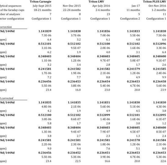
on the newer generation of Triton™ (i.e. Triton Plus™ from LMV). This means that absolute ratios should not be compared between instruments when investigating variations at the 5 to 10 ppm levels. These residual differences can of course be suppressed by looking at relative ratios instead of absolute values. Given that the sources of the residual differences are related to the instrument itself and to the deterioration stage of the faraday cups, we divided our JNdi-1 dataset into five groups (cf. Table 4) to calculate the relative variability in isotope ratios (µ values) shown in Figure 9. A group gathers data collected on the same instrument and over a period of 4 months maximum.

4.1.3.b. Uncorrected vs. drift-corrected dynamic Nd isotope ratios

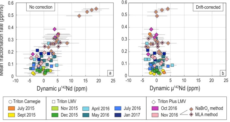
The effects of the drift-correction on dynamic Nd isotope ratios can be evaluated by comparing absolute ratios as in Tables 3 and 4, or relative µ values as shown in Figures 9 and 10. Figure 9a confirms the expected relationship between the rate at which Nd fractionates during a run and the resulting dynamic 142_Nd/144_{Nd ratios. The deviation of the compositions}

towards higher than true values (i.e. µ142 > 0) for high fractionation rates is consistent with our

cup configurations as explained in Section 4.1.2. More importantly, we note that processing the standards through chemistry results in higher fractionation rates, and hence significantly increases the risk of shifting the dynamic ratios towards high µ142 values. Such behavior is

particularly obvious when comparing unprocessed JNdi-1 Nd standards to those measured during the same analytical sequence, but processed through different chemistries following the MLA or NaBrO3 methods (cf. pink diamonds in Figure 9a). Standards having the highest

fractionation rates also have the highest 142Nd excesses, up to +19 ppm according to our measurements. This suggests that samples may be more likely affected by drift effects than unprocessed JNdi-1 standards generally used to evaluate the accuracy and the precision of Nd measurements. This may be due to the presence of organic residues from the resin and/or to the lower amount of Nd analyzed in samples compared to unprocessed JNdi-1 standards. Using unprocessed JNdi-1 standards to evaluate the quality of Nd isotope analyses may lead to an underestimation of the accuracy and precision of the dynamic compositions of the samples, unless drift effects are accurately corrected. In Figure 9b, the drift-correction efficiently eliminates the large positive µ142 biases of standards having high mean

fractionation rates, up to 0.6 ppm/s, and does not over-correct standards having mean fractionation rates close to zero. Similar efficiencies were observed for other dynamic Nd isotope ratios (see Appendix A and B, Tables 3 and 4), suggesting that the drift-correction enhances the accuracy of the measurements. The drift-correction also generally improves the