Distributed mode estimation through constraint decomposition

Distributed Mode Estimation

Through Constraint Decomposition

by

Henri Badaro

ARCHIVES

OCT 18

2010

L IBP

JR FS

Submitted to the Department of Aeronautics and Astronautics

in partial fulfillment of the requirements for the degree of

Master of Science in Aeronautics and Astronautics

at the

MASSACHUSETTS INSTITUTE OF TECHNOLOGY

September 2010

@

Massachusetts Institute of Technology 2010. All rights reserved.

Author ...

Department of Aeronautics and Astronautics

August 23, 2010

Certified by ...

Brian C. Williams

Professor

Thesis Supervisor

A ccepted by ...

.... .

. ..

. .

--...

. .

--Eytan H. Modiano

Associate Professor of Aernautics and Astronautics

Chair, Committee on Graduate Students

Distributed Mode Estimation

Through Constraint Decomposition

by

Henri Badaro

Submitted to the Department of Aeronautics and Astronautics on August 23, 2010, in partial fulfillment of the

requirements for the degree of

Master of Science in Aeronautics and Astronautics

Abstract

Large-scale autonomous systems such as modern ships or spacecrafts require reliable monitoring capabilities. One of the main challenges in large-scale system monitor-ing is the difficulty of reliably and efficiently troubleshootmonitor-ing component failure and deviant behavior. Diagnosing large-scale systems is difficult because of the fast in-crease in combinatorial complexity. Hence, efficient problem encoding and knowledge propagation between time steps is crucial. Moreover, concentrating all the diagnosis processing power in one machine is risky, as it creates a potential critical failure point. Therefore, we want to distribute the online estimation procedure. We introduce here a model-based method that performs robust, online mode estimation of complex, hard-ware or softhard-ware systems in a distributed manner. Prior work introduced the concept of probabilistic hierarchical constraint automata (PHCA) to compactly model both complex software and hardware behavior. Our method, inspired by this previous work, translates the PHCA model to a constraint representation. This approach handles a more precise initial state description, scales to larger systems, and to allow online belief state updates. Additionally, a tree-clustering of the dual constraint graph associated with the multi-step trellis diagram representation of the system makes the search distributable. Our search algorithm enumerates the optimal solutions of a hard-constraint satisfaction problem in a best-first order by passing local constraints and conflicts between neighbor sub-problems of the decomposed global problem. The solutions computed online determine the most likely trajectories in the state space of a system. Unlike prior work on distributed constraint solving, we use optimal hard constraint satisfaction problems to increase encoding compactness. We present and demonstrate this approach on a simple example and an electric power-distribution plant model taken from a naval research project involving a large number of modules. We measure the overhead caused by distributing mode estimation and analyze the practicality of our approach.

Thesis Supervisor: Brian C. Williams Title: Professor

Acknowledgments

I would like to express my gratitude to the people who supported and helped me

through to the completion of this thesis.

I am grateful to my advisor and thesis supervisor, Brian Williams, for his key

insights and encouragements on my research, his critical help on technical writing, and for his efforts to make the thesis deadline.

I would like to thank and congratulate my parents, my brother, and the rest of

my family, whose constant love, support, and friendship allowed me to achieve what I have achieved so far, including this Master's thesis.

I would also like to thank all my friends and labmates who helped me during

the research, writing, completion, and printing phases of this thesis, in particular: Shannon, Alborz, Andreas, Cristi, David, Hiro, Hui, Julie, Patrick, Ted, Yi. Thank you to Alison for the logistics, Dave, Mike and Paul for the the meetings, Bobby, Larry, Seung and Stephanie for their company in the lab.

I would finally like to thank my friends from MIT and the ones whom I knew before, for the endless conversations, for the off-campus moments, the great fun, and the support. They made my stay here so valuable and unforgettable, in the dorms, Cambridge, and remotely from other places and time zones. We will stay in touch by way of aeronautics, TCP/IP or UDP.

This research was sponsored by a grant from the Office of Naval Research through the Johns Hopkins University Applied Physics Laboratory, contract number

Contents

1 Introduction 17

1.1 Motivation... . . . . . . . . 17

1.2 Challenges and Required Capabilities . . . . 18

1.3 Approach and Innovations . . . . 20

1.4 O utline . . . . 21

2 Related Work 23 2.1 Distributed Diagnosis and Constraint Solving . . . . 24

2.1.1 Previous Work in Distributed Diagnosis . . . . 24

2.1.2 General Distributed Constraint Optimization Methods . . . . 27

2.1.3 Distributed Optimal Constraint Satisfaction . . . . 28

2.2 Model Representation and Problem Encoding . . . . 29

2.3 Online Mode Estimate Update . . . . 31

3 Problem Formulation 33 3.1 O bjective . . . . 34

3.2 Model-Based Diagnosis Problem . . . . 34

3.2.1 Input: Probabilistic Plant Model... . . .. . ... 35

3.2.2 Input: Commands . . . . 38

3.2.3 Input: Observations . . . . 38

3.2.4 Parameter: Number of Steps . . . . 39

3.2.5 Parameter: Number of Candidates . . . . 39

3.3 Assum ptions . . . .

3.4 Realistic Example . . . . 3.4.1 Component Description... . . . . . . . ..

3.4.2 Component Dynamics.. . . . ..

3.4.3 Monitoring Problem . . . .

3.5 Optimal Constraint Problem.... . . . . 4 Distributed Optimal Constraint Satisfaction Problem Solving

4.1 M ethod Overview . . . . 4.2 Problem Decomposition . . . .

4.2.1 Constraint Graph . . . . 4.2.2 Tree Clustering into an Acyclic Graph . . 4.2.3 Graph Simplifications . . . . 4.2.4 Choice of a Root . . . . 4.2.5 Adding Costs to Nodes . . . . 4.3 Distributed Problem Solving . . . . 4.3.1 Binary Tree Structure . . . . 4.3.2 Pairwise-Optimal Solution Enumeration 4.3.3 Search Bound and Termination Condition 4.3.4 Best-First Enumeration Overview . . . . . 4.3.5 Simple Conflict Handling . . . . 4.4

4.5

Difficulties of Exploring Different Variable Assignments in Parallel . Sum m ary . . . .

5 Modeling and Estimation Problem Framing 5.1 Model Representation . . . .

5.1.1 Prior Work and Requirements . . . . 5.1.2 Hypotheses . . . .

5.1.3 Modeling Language . . . . 5.1.4 Innovation in the Modeling Capabilities. .

5.2 Problem Formulation . . . . 50 ... ... 50 . . . . 51 . . . . 58 . . . . 62 . . . . 64 . . . . 66 . . . . 68 . . . . 69 . . . . 72 . . . . 75 . . . . 78 86 88 91 92 92 93 94 97 100

Output of the Problem Formulation . . . . Trellis Diagram Expansion . . . . Model to Constraint Problem Detailed Mapping . . . .

Mode Estimation Problem Framing . . . . Trajectory Update.... . . . . ..

Belief State Update Algorithm . . . . Recovery from False Hypotheses . . . .

6 Real-World Mode Estimation Implementation and Analysis

6.1 Experimental Results . . . . . 109 6.1.1 Implementation . . . .

6.1.2 Simple Inverter Example . . . .

6.1.3 Electrical Power Distribution System . . . .

6.1.4 Estimation Scenario.... . . . . . .. 6.1.5 R esults . . . .

6.2 Analysis and Possible Optimizations . . . . 6.2.1 Problem Size and Complexity . . . .

6.2.2 Discussion on Hierarchy . . . .

6.2.3 Choice of N and K . . . .

7 Conclusion and Future Work

7.1 Future W ork . . . .

7.1.1 Improvement on Modeling and Encoding . .

7.1.2 Probabilistic Behavior Representation . . . .

7.1.3 Hybrid Continuous and Discrete Estimation

7.2 Conclusion . . . .

A Simple Inverter Model

B Power Distribution Plant Model 5.2.1 5.2.2 5.2.3 5.2.4 5.3 Belief 5.3.1 5.3.2 100 101 101 105 107 107 108 109 110 110 111 111 112 115 115 115 116 119 119 119 120 121 121 123 125 . . . . . . ... . . . .

List of Figures

Redundant Power Distribution System Model Model of the behavior of a relay . . . . Primal Graph Example . . . .

Dual Constraint Hypergraph Example Variable-Constraint Duality Example Tree Clustering Example . . . . Local Cost Computation . . . .

Double Structure Pairs-Subrees . . . . Node Communication... . . . . . . .

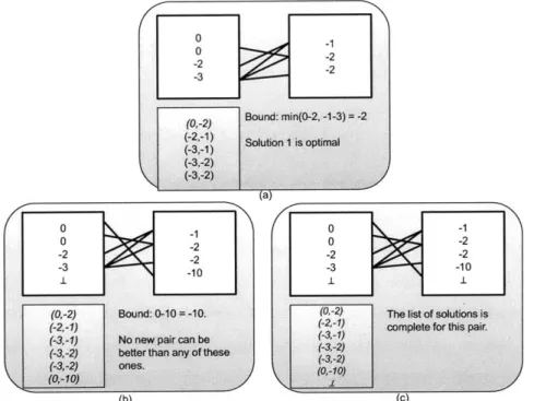
Valid Pair Solutions . . . . 4-9 Best-First Enumeration Diagram . .

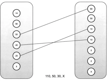
4-10 Pairwise Solution Matching Example: 4-11 Simple Conflict Checking . . . .

Computation of Costs . . . . 3-1 3-2 4-1 4-2 4-3 4-4 4-5 4-6 4-7 4-8

.. .. ..

...

.. .. ..

...

Definitions and Examples

1 Model-Based Diagnosis Problem . . . . 35

2 Plant M odel . . . . 36

3 Com ponent . . . . 36

4 Transition... . . . . . . . . . . . 37

5 Branch... ... 37

6 State Trajectory . . . . 40

7 Optimal Constraint Satisfaction Problem. . . . . . . . . 45

8 CSP Primal Dual Constraint Graph... . . . . . . . 52

9 CSP Dual Constraint Hypergraph . . . . 54

10 CSP Dual Binary Constraint Graph . . . . 55

11 Subproblem .. . . . . . . . 70

12 Probabilistic, Hierarchical Constraint Automaton . . . . 95

13 Transition Structure . . . . 97

List of Algorithms

1 Constraint Graph Building Algorithm . . . . 58

2 Constraint Graph Building Algorithm . . . . 60

3 Problem-Merging Algorithm . . . . 64

4 Root-Choice Algorithm . . . . ... . . . . . . . . . 65

5 Best-First Enumeration Non-optimality Condition . . . . 77

6 Pair-Level Best-First Enumeration 1/2 . . . . 79

7 Pair-Level Best-First Enumeration 2/2 . . . . 80

Chapter 1

Introduction

1.1

Motivation

Large-scale autonomous systems such as modern ships and spacecraft require reliable monitoring capabilities. Unmanned vehicles are not the only devices to employ au-tonomy. As air, sea, and ground vehicles become more complex, they also require a

high level of autonomy to assist the users, pilots, or operators.

For instance, in a large modern ship, complex systems ensure the proper distri-bution of water, power, heat, air, and information. There may be several reasons to limit the amount of human intervention in these systems. Humans, particularly when under pressure, are error-prone. Moreover, some critical zones of a vehicle may not be accessible or can be dangerous due to steam, high voltage, and water leaks. Therefore, robust autonomy capabilities are crucial to increase vehicle survivability where human intervention is not possible or responsive enough.

Autonomous embedded systems, such as distribution systems in intelligent vehi-cles, may fail in various predictable or unexpected ways. Therefore, a robust auton-omy capability requires reliable monitoring methods. Moreover, if relevant diagnosis and troubleshooting can be performed, more complex and capable systems can be used while maintaining the same level of survivability.

System diagnosis consists of identifying sets of working and faulty components, and their probability. An autonomous diagnosis engine analyzes commands and

obser-vations of the system in order to output diagnoses over time. Autonomous diagnosis allows to detect problems without human intervention, hence increasing safety.

Yet, if the diagnosis engine fails, the whole mission is in jeopardy. Therefore, centralizing the diagnosis puts the system at risk: by concentrating all the computing and decision making into one place, a critical failure point is created. A way to solve this problem is to distribute the diagnosis process. Furthermore, if this process is distributed across several machines, one can still duplicate each of them. If each cluster (computer, or processor) is redundant, the whole system fails only when two paired clusters fail, whereas if a centralized (monolithic) system is duplicated, two failures are sufficient to endanger the computational process.

1.2

Challenges and Required Capabilities

Autonomous monitoring of embedded systems, such as the ones previously mentioned, raises a number of challenges, which can be addressed by extending the current state of the art in distributed diagnosis [15, 19, 13, 36, 21, 14].

The first challenge comes from the complexity of the system state space, in par-ticular if a system consists of both software and hardware components. The state space representing the possible nominal and unknown behaviors grows much faster than the number of components. Therefore, a monitoring process may not be able to enumerate exhaustively all possible diagnoses in a reasonable amount of time. For these complex systems, an efficient problem encoding may be a crucial step in making the search of component failures tractable.

The second major challenge concerns the dynamic behavior of the systems we are monitoring. These embedded systems evolve over time, and the components may be in various states across the period of observation. However, starting a new estimation process at every time step without keeping track of previous intermediate results is both time consuming and inefficient. A system state is estimated from a history of previous observations. Therefore, in the case of long experiments, it is interesting to update the belief state while keeping as many previous estimates and as much

knowledge of the system as possible.

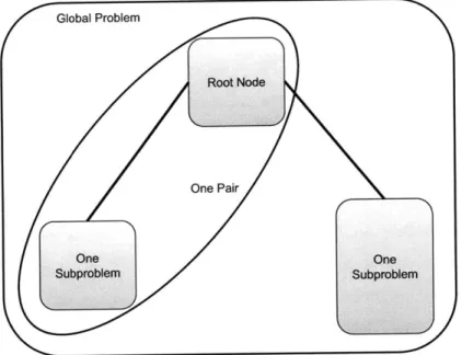
Finally, a third important challenge has to do with the distribution of the monitor-ing process. If we want to solve the diagnosis problem online in a distributed way, we need to decompose it and decentralize it onto several computing clusters. Therefore, we need a decomposable problem framing, paired with a distributed optimal solver. One of the main difficulties of performing a robust diagnosis lies in the fact that we do not only look for a single most likely diagnosis, (as this would not be robust to diagnosis error). We must compute a whole set of optimal solutions in a distributed way, while limiting the amount of communication between the clusters.

Distribution is an important step for improving monitoring reliability. The ad-ditional robustness associated with distribution can be interpreted in several ways. First, in the case where a computation node is lost, a distributed and decentralized diagnosis algorithm may still be able to work in a degraded mode, providing most likely diagnoses to the best of the knowledge of the remaining cluster. This is indeed the case for our approach: it can still provide diagnoses even if some computers or some observations are not available. Yet, we do not deal with cases where failing means of communication lead to corrupted message transmission.

Second, if each computer is duplicated in a distributed monitoring process, the only way to make the whole computation fail is to lose two identical nodes. The loss of two non-paired nodes does not affect the monitoring ability. On the other hand, if a large computer centralizing all monitoring is duplicated, the loss of two machines destroys all the monitoring capability. Therefore, in order to reach the same level of tolerance to computer failure as in a distributed process, it may be necessary to add more than one large backup computer in the centralized version. Hence, if the online estimation process is distributed onto several processors, then the same level of robustness to processor or communication failure requires less redundancy.

Finally, with a suitable encoding, estimation may be dispatched locally and gath-ered to determine the overall system state. This permits the diagnosis of embedded systems where several subsystems are integrated from different manufacturers, in the sense that this distributed algorithm could be adapted to perform several partial local

mode estimations specific to each component in order to achieve global monitoring.

1.3

Approach and Innovations

In order to provide the three main required capabilities introduced in Section 1.2, we propose a method to estimate in a distributed manner the system state evolution over a certain time window. We also propose a way to update this belief of the system state when new observations are made. Hence, we introduce a capability to monitor a mixed hardware and software large-scale system over long time periods, by distributing the required processing power on a set of computers.

For that purpose, we improve and extend a model-based approach to diagnosis that uses Probabilistic Hierarchical Constraint Automata (PHCA) modeling to per-form mode estimation over a window of N time steps [27]. This method handles multiple faults, novel faults, intermittent faults, and delayed symptoms. We increase the scalability of this method by encoding the estimation problem as an Optimal Constraint Satisfaction Problem (OCSP) containing only hard constraints and costs on some single variable assignments [42]. An increased scalability allows us to solve larger problems and hence deal with complex systems with mode components.

Every time step, new observations of the system are made, and new commands are sent. The state of the system evolves and its diagnosis must be updated accordingly. If diagnoses are performed over a moving, finite, time window of operations, a belief state update consists of an update of the estimated state trajectories of the system. In order to allow an efficient belief update at each new time window, we introduce a dummy decision variable into this OCSP. This variable summarizes the previous most-likely finite horizon diagnoses along with their probabilities. Depending on the new observations, some of these previous hypotheses will be extended to produce updated estimations on the most likely system state trajectories.

Most importantly, the distribution of the mode estimation process is ensured by a distributed optimal solver that enumerates solutions to the aforementioned OCSP in a best-first order, hence allowing us to compute the K most likely diagnoses at

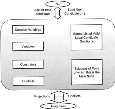
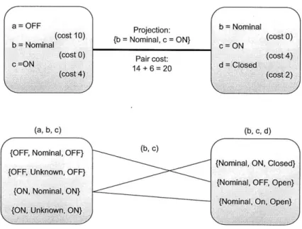
each time step. This method uses the optimal solver OPSAT in each cluster [42], and the clusters work on a tree-decomposed version of the dual constraint graph of the OCSP. Clusters communicate by passing messages informing their neighbors of their partial solution candidates or by sending conflicts to signal dead-ends in the search. This algorithm is inspired by a previous message passing method that uses only soft-constraints [29], but our method focuses on increased scalability by using hard constraints and by introducing conflict handling.

To summarize, our approach has three sources of innovation:

1. distributed optimal hard-constraint problem solving,

2. efficiency of a problem encoding, and

3. the ability to update the belief state of a system online.

This approach will be presented on simple examples and on a realistic power distribution system example detailed in Chapter 3. This latter large-scale model contains many components that can fail in unexpected ways. It is taken from a larger naval project, where robust autonomy is crucial for survivability, and to reliably add

additional functionality to embedded systems.

1.4

Outline

The rest of this thesis is organized as follows.

In Chapter 2, we first describe relevant prior work in the fields of distributed di-agnosis, distributed optimal constraint solving, and model-based estimation. We also discuss how this work tackled some of the challenges mentioned in this introduction. We then present a problem statement and a motivating large-scale power distribu-tion system example in Chapter 3. This example is a real-world scenario that justifies the choice of methods and the orientation of this research to achieve distributable, robust mode estimation.

The subsequent three chapters explain our approach, innovations, and technical solutions. Our approach to distributed model-based diagnosis consists of two phases.

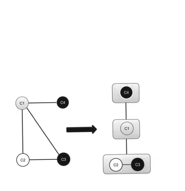
First, a model of the system is used to frame the diagnosis problem into a stan-dard optimal constraint satisfaction problem. This problem is decomposed with an off-the-shelf tree-decomposition method, in order to produce a tree of connected sub-problems. Then, the second phase performs online diagnosis by solving the tree of subproblems in a distributed manner. The distributed search of solutions outputs a set of most-likely state trajectories depending on observations and commands. The distributed search over the coarse-grain decomposed problem consists of sequences of local optimal solution enumerations, and communications of these solutions between neighbor subproblems by message-passing. Additionally, the state estimates may be updated at each time step. Empirical results show that model-based diagnosis can be performed on large-scale systems and that our diagnosis engine can detect unpre-dicted failures. Moreover, the overhead on processing time of a distributed search against a centralized search is small, even if it is measured on a simulated distributed optimal constraint solver.

Chapter 4 proposes a novel distributed search method based on tree-decomposition of a dual hard-constraint graph. Chapter 5 deals with an improved model and problem encoding of probabilistic hierarchical constraint automata, which allows us to update the mode estimates of a system more efficiently than in prior work. Next, Chapter

6 introduces implementation insights and empirical results for the distributed mode

estimation method.

Chapter 2

Related Work

In Section 1.2 we introduced three challenges that arise from autonomous, distributed diagnosis of large-scale embedded systems, and we presented three features that a diagnosis executive could deliver in order to tackle these three challenges.

First, the executive should run on a decentralized set of computers, without jam-ming the network with excessive intermediate result communication. In Section 2.1, we describe related work in distributed diagnosis and distributed optimal constraint solving. The objective of this distribution is to avoid centralizing all the computing power at one single point.

Second, we want to diagnose mixed software and hardware embedded systems that may disclose unexpected behavior. In Section 2.2 we describe methods often used to represent models of embedded systems and to encode the diagnosis problem, in the field of model-based diagnosis. These methods mainly use probabilistic and hierar-chical automata in order to model finite-domain systems with a discrete stochastic state evolution.

Finally, mode estimation should be able to keep as much information as possible, while updating the mode estimates at each new discrete time step. In Section 2.3, we discuss previous methods used to propagate knowledge of the system behavior and previous estimates over time when new observations are made and new commands are sent. As the number of possible state evolutions is very large, monitoring executives are often not able to keep track of the whole evolution history, therefore an improved,

more efficient problem framing is needed.

2.1

_{Distributed Diagnosis and Constraint Solving}

In this section, we present work related to distributed diagnosis. Many diagnostic methods rely on a constrained optimization process. Hence, distributed diagnosis can be achieved by decomposing the online problem solving. This is why we also recall techniques commonly used to decompose and solve general constrained optimization problems. Finally, we focus on more specialized methods for dealing with distributed discrete optimal constraint satisfaction.

2.1.1

_{Previous Work in Distributed Diagnosis}

One of the most direct ways to perform distributed diagnosis is to use and modularity of the problem framing. To perform decomposition, this kind of approach can be found in expert diagnostic systems [19]. For the systems we care about, expert system diagnosis offers a less powerful diagnostic capability than the more modern model-based approach. However, by nature, expert diagnosis can perform large-scale simple distributed diagnoses with a small overhead as compared to a centralized version.

Expert diagnosis uses knowledge about the system to efficiently associate obser-vations to diagnoses [19]. This knowledge can be based on a series of simulations or benchmarks. Additionally, humans can provide the system with knowledge about the different failure scenarios. Case-based and rule-based reasoning systems are particu-larly useful solutions when a model of the system is not known. Moreover, rule-based systems are capable of exploiting a large amount of parallelism, due to the nature of the constrained problems involved [15]. These monitoring systems are based on lists of simple implication rules for checking whether the behavior of components is consistent with predefined descriptions, and so the truth of each of these implications can be verified independently on different machines.

Simple rule systems are standard paradigms for space systems. When scaling on large systems, the rule sets may become too large to maintain or to debug. Moreover,

powerful as it may be, a knowledge-based approach does not deal with unexpected or unpredictable behaviors of system components. Hence, in cases where a complete expertise is required, model-based diagnosis has been proposed in order to increase robustness to unexpected behavior. Model-based diagnosis uses a model of the system and the environment along with observations to determine if the estimated behavior is consistent with a nominal or an unknown situation.

In spite of the practicality of rule-based diagnosis when it comes to distributed computation, it may not apply for our usage, as we want to determine the probabilities of each diagnosis.

Most previous distributed model-based diagnosis methods were conducted in the field of multi-agent systems.

Fabre et al. [13] present a distributed diagnosis method for large, discrete-event, dynamic systems. The motivating idea of this paper is to deal with systems that are too large to be handled as a whole. The method proposes that local supervi-sors provide partial local monitoring, in a framework related to Markov fields theory and Bayesian networks. A global system is factored into smaller subsystems that communicate through common variables. Then a monitoring executive fully uses concurrency properties to identify independent behaviors, so as to limit the problem complexity. Additionally, this method is fully fast, decentralized, and it is robust to message passing latency. This method however cannot output a set of most-likely state trajectories, it stops when one consensus on a globally-consistent diagnosis is reached between all the neighbors. In order to provide robustness to our system, we cannot limit ourselves to one single diagnosis per time step.

Roos et al. [36] analyze the influence of spatial and semantical knowledge dis-tribution while performing multi-agent diagnosis. Multiple agents, each having their own local constraints, interact with each other, creating other interaction constraints. Hence, Ross et al. conclude that the sole knowledge of information in partial problems is not sufficient to decide what a global situation looks like. As we also notice in this thesis, when solving decomposed optimal constraint satisfaction problems, that the way knowledge and interactions are distributed among components has a substantial

influence on the difficulty to reach consensus between subproblems. Therefore, as pointed out by Roos et al. [36], though theoretically possible, multi-agent or dis-tributed diagnosis are not necessarily always practically feasible.

Because of the aforementioned spatial knowledge distribution issues, other meth-ods have analyzed the influence of the topology of a distributed system on the dis-tributed diagnosis paradigms. This insight is particularly valuable in networked em-bedded systems In these systems, the topology of the system network determines the shape of a diagnosis engine. Hence, Kurien, Koutsoukos and Zhao in [21] use model-based diagnosis along with network topology analysis to perform consistency-based diagnosis. This method produces distributed constraint satisfaction problems shaped by the network topology. Furthermore, this diagnosis approach is fast. Yet, it does not take into account the probability of component failure. Instead, it returns diagnoses that are consistent with the observations. Hence, it may overestimate the likelihood of a multiple failure for instance, if this multiple failure explains a deviant device behavior.

Finally, another active field of research is based on Petri net representation, such as in [14] by Genc and Lafortune. Petri nets can model the possible evolution of discrete-event systems, and they are backed up with a theoretical mathematical model that allows many computational optimizations. In [14], this abstraction method is used to perform online model-based fault diagnosis. In this method, one Petri net is decomposed into two entangled nets, which lead to a distributed monitoring process-ing. The theory behind Petri nets remains valid and can still be used in each of the sub-nets after the decomposition; therefore, the problem decomposition and distribu-tion is computadistribu-tionally efficient. This method assumes that the Petri nets models of the system can be decomposed into two place-bordered Petri nets satisfying certain conditions, so that the two resulting diagnosers can exchange messages about the occurrence of observable events.

2.1.2

General Distributed Constraint Optimization Methods

Many model-based diagnostics processes can be framed as constraint optimization problems [10, 39, 40]. A probabilistic model of the software and hardware components of the system along with observations can be used to monitor the system behavior

by computing the most likely states. These are determined from the optimal feasible

solutions to the estimation problem.

We assume in this work that the variable domains are discrete, as well as the divisions of time into synchronous time steps. This influences the problem represen-tation and the solution method. Many systems, such as digital electric circuits or sequential mechanical devices, operate over a finite number of discrete modes, and thus can be well represented by a discrete model. Moreover, the behavior of sequen-tial devices whose components which modes evolve at similar synchronous speeds can be adequately captured with discrete time steps. However, very non-linear dynamical systems, such as heat machines or turbulent fluid circuits, are unlikely to be modeled with discretized steps.

Our problem may be framed as a standard mixed integer-linear program [5] that can be distributed with a method like Dantzig-Wolfe decomposition [8] (Column Generation) adapted to MILPs. Although a MILP framing is not the most convenient for our purposes, it is worth mentioning, as some notions in the decomposition method can be found in later more specialized approaches, such as master problems (objective function to optimize), coupling constraints, projections, or cutting planes (which are a kind of conflicts).

A more specialized and adapted framework is mixed linear-logic programming.

This kind of problems can be solved using Bender's decomposition [3, 18] (row gener-ation), which shares many similarities with the Dantzig-Wolfe method, including the generation of candidate solutions and cutting planes. More recently, J6gou, Terrioux and Pinto [20, 32] have presented computationally efficient and practical distribution algorithms for optimal constraint satisfaction problems, adapted to fast, distributed diagnosis. However all these methods directly allow to find a single solution.

2.1.3

Distributed Optimal Constraint Satisfaction

In general, constraint optimization problems (with soft constraints) can be solved

by distributed constraint optimization methods (DCOP). Many available algorithms

have been optimized for various particular problems. For instance the multiple knap-sack problem or the distributed graph coloring problems can indeed be solved effi-ciently by DCOP algorithms, but the generic DCOP algorithms have higher average complexity than their specialized counterparts. They are either exponential in mem-ory space (Distributed Pseudotree Optimization Procedure in [31]) or exponential in the number of messages exchanged between agents (Asynchronous Backtracking in

[30], Asynchronous Partial Overlay in [22], No-Commitment Branch and Bound in [6]).

If a large amount of memory is available, DPOP may look promising in our case, as it bounds the need for communication between agents, and it can solve OCSP problems efficiently. However it only allows to find the optimal solution of a problem. It is indeed possible to find the next optimal solutions by negating all the previous assignments inside new constraints. However this kind of constraint involving all the variables would affect the efficiency of the decomposition by creating a fully connected pseudo-tree. Moreover, constraints are expressed in terms of a set of possible partial assignments. Thus a negative constraint is transcribed as the set of all the other possible partial assignments in the scope of the negation. This enumeration leads to an exponential number of possibilities, and if all the variables are involved, the constraint description is too large to be represented.

We chose a method similar to the one described by Sachenbacher and Williams in [37] that can compute a set of optimal solutions to an optimal soft-constraint satisfaction problem (valued CSP). In this thesis, we use hard constraints instead of soft constraints because our online mode estimate update method is based on a hard-constraint encoding. Additionally, we inspired from this previous method and increased its scalability on larger problems in order to adapt it to our needs, by using a coarse-grain problem decomposition.

Our approach applies a tree-clustering method [11] to the dual graph of hard con-straints in order to produce a tree of partially correlated sub-problems. We then use a conflict-based best-first enumeration of the solution to compute globally consistent trajectories in the transition space by passing messages and conflicts between neigh-bor sub-problems. It is a more specialized technique than the ones in the previous subsection to solve discrete problems. And as we restrict our encoding to hard con-straints, we manage to increase the efficiency of our method compared to the one by

Sachenbacher and Williams [37].

2.2

Model Representation and Problem Encoding

In a physical system, some faulty component behaviors may not be immediately visible when failure occurs. For instance, it is not possible to distinguish a relay that is stuck-closed from a properly working closed relay until it is sent a command to toggle open. Hence, symptoms of a failure may arise some time after the failure actually occurs. This is why we need to estimate the state of a system over a history of observations (finite time window), as explained later in this section.

Moreover, we need to be able to accurately represent the possible evolutions of the components of the system. Thus, we need a diagnosis problem formulation that takes into account the probabilistic (stochastic) behavior of a system. We want to take into account the probability of failure of each component because it is not com-putationally possible to compute all the possible diagnoses at every time step. Hence, we choose to enumerate the most-likely diagnoses, maximizing the probability that the accurate diagnosis is in the set of enumerated solutions. That is why we need to take probabilities into account in our model representation.

In the model-based monitoring framework, several automaton-based representa-tions have been used to model a system. When dealing with dynamic systems, these models are usually encoded into intermediate representations such as a trellis diagram. Probabilistic Concurrent Constraint Automata (PCCA) were first introduced in the Livingstone and Titan mode estimation frameworks [41, 40]. They are used to

rep-resent plant models by modeling each component as a concurrent automaton. These components can interact with each other and their behaviors is not deterministic.

PCCA could not model software behavior.

In order to offer a more expressive modeling than PCCA, previous work introduced a mode estimation method framing a compact Probabilistic, Hierarchical, Constraint Automaton (PHCA) representation into a soft constraint optimization problem [28]. However it did not allow an efficient use of complex transitions or the definition of an initial state, both desirable to achieve a much more accurate modeling.

Additionally, this method introduced a finite-time-horizon mode estimation. N-step time window problem encoding introduced in this previous work is a necessary feature that we are keeping in our approach. Finite time window mode estimation diagnoses systems by keeping track of observations and commands over a finite history of time steps.

In this thesis, we effectively propose a method for an efficient, PHCA-based encod-ing of complex transitions that mix probability distributions with constraint guards. We also propose a way to deal with initial state representation. Instead of specifying a single possible initial state as in the previous work, we can specify a probability distribution over a set of initial states. Each initial state corresponds to a certain set of modes for each component of the system. Hence, we intend to represent as precisely as possible a probabilistic evolution of a model while remaining tractable.

In the method presented in this thesis, the system representation as a probabilis-tic hierarchical constraint automaton handles complex transitions and specifies an initial probability distribution over the possible system states. This encoding is then converted into a more compact multi-step trellis diagram, then framed as an opti-mal constraint satisfaction problem. These notions will be more foropti-mally defined in later chapters. In short, the trellis diagram represents all the possible sequences of transitions between feasible states from an initial to a final time step.

Automata representations are not the only way to model systems in the framework of model-based diagnosis. For instance, the model-based approach in [1] by Armant, Dague and Simon that deals with distributed consistency-based diagnosis is focused

on theory representations. These encodings aim at providing efficient extractions of minimal diagnoses.

2.3

Online Mode Estimate Update

If the systems to diagnose are static, like the ones covered by the Sherlock-style mode

estimation [10], there is no need to update the mode estimate. In this thesis, we are dealing with dynamic systems that evolve over discrete time steps, and we want to integrate new observations each time step to monitor the system evolution.

The approach of Martin, Chung and Williams in [23] improves the accuracy of transition probability computation compared to the regular PHCA estimation by us-ing observation functions, whereas this thesis focuses on a tractable simplified repre-sentation and encoding of transitions. This paper extends the Best-First Belief State Enumeration (BFSE) with the Best-First Belief State Update method (BFBSU) [24]

by eliminating a simplification concerning the observation probability distribution.

The improvements in their work and the improvements in this thesis are not mutu-ally exclusive, but we chose to focus on the scalability of the computation for large models, such as the one presented in the next chapter.

As compared to Mikaelian, Williams and Sachenbacher in [28] who propose to recompute the mode estimates, or belief state, for a whole time window at every new time step, in this thesis we keep track of the previous state trajectories to extend them

by one time step every new time step. We first compute enabled transitions, then

append some previously computed trajectories at each time step so that a predefined number of most-likely estimates can be computed. Therefore, our approach needs two passes of constraint optimization, as explained in Chapter 5, one to compute transitions, and one to decide which trajectories can be extended according to the new observations.

Now that we have presented some background and related work about distributed mode estimation, we will more precisely state the problem that we tackle in this thesis in Chapter 3.

Chapter 3

Problem Formulation

This chapter formally describes the problem of distributed mode estimation of dis-crete dynamic systems. Model-based diagnosis of embedded systems can be achieved through a method called mode estimation. Mode estimation considers that system components can probabilistically transition between several behaviors, or modes. Its objective is to determine the hidden state of the system in the form of the set of com-ponent modes. Estimation accuracy is key to troubleshooting failures, should they occur, with the best likelihood possible. For instance, a broken relay and a broken power supply may both explain a system failure; and if power supplies are known to be more reliable than relays, without additional information, the diagnosis: "the relay is broken" may be more likely than: "the power supply is broken".

We first present the objective (Section 3.1) and the inputs and outputs to our mode estimation problem (Section 3.2). Then in Section 3.3, we discuss the assumptions and hypotheses of the problem, and we propose a motivating example (Section 3.4). As specified earlier in our approach in Chapter 1, the diagnosis problem is formu-lated internally into a series of a constraint optimization problem. Hence, distributed diagnosis is achieved by solving this constraint problem in a distributed manner. Therefore, Section 3.5 formally defines the kind of optimal constraint problem we need to decompose and solve.

3.1

Objective

Mode estimation capabilities may be added to systems such as a power distribution circuit in order to perform diagnosis. More precisely, we want to perform distributed

N-step, K-best mode estimation through the tree-decomposition of the dual

con-straint graph of the diagnosis problem.

Let us consider a simple electronic gate with three modes: wire, inverter, and

unknown. Each of these modes corresponds to a behavior. In the wire mode, the

input equals the output, whereas in the inverter mode, the output and the input have opposite boolean values. Finally, the last mode, unknown is unconstrained. It represents any possible situation, such as the case where the output is stuck to 1 or

0. This gate can receive a sequence of commands to switch between nominal modes,

and commands may fail with a certain probability. The objective of distributed mode estimation is to be able to evaluate the most likely possible evolutions of this circuit, depending on the failure probabilities of the model, and observations. A set of diagnoses is updated at each time step, and the computation power needed to solve this diagnosis problem is distributed on several computers.

In the next section, we define more formally the inputs and outputs of the moni-toring problem.

3.2

Model-Based Diagnosis Problem

The main input to our model-based diagnosis system consists of a probabilistic plant model example (3.2.1), a set of commands sent at each time step to the plant (3.2.2), and observations sent at each time step by the plant (3.2.3). Other user parameters are also fed to the system: the size of the diagnosis time window (number of steps of the time window, 3.2.4), and the number of candidate diagnoses to compute at each belief state update (3.2.5).

The main output is a diagnosis in the form of a set of most likely state trajectories

0.3 : (relayi is open, relay2 is closed)timei, (relayi is closed, relay2 is broken)time2 The objective of this thesis is to present a distributed method that computes a set of most likely state trajectories. To that extent, we choose to frame this problem into an optimal constraint satisfaction problem and solve this problem in a distributed manner. An OCSP is a hard-constraint satisfaction problem in proposition state logic with an associated objective function. OCSP's will be formally defined in Section 3.5. Definition 1 (Model-Based Diagnosis Problem)

A model-based diagnosis problem is a quintuplet

(Plant-_Model, Commands, Observations, N, K)

where

1. PlantModel represents the set of system components and their interactions (Subsection 3.2.1);

2. Commands = {ci, CnumberOfCommands} models the set of commands sent to

the system;

3. Observations {01, ..., CnumberOfObservation3} contains the sensor data

(Subsec-tion 3.2.2);

4. N is the size of the observation history used to monitor the system (Subsection

3.2.4); and

5. K is the number of state trajectories to compute (Subsection 3.2.5). o

3.2.1

Input: Probabilistic Plant Model

The core of a model-based diagnosis method is a plant model representation. In this thesis, we deal with probabilistic representations, as we look for the most likely diagnoses. The plant model describes all the components (also called modules), their interactions, inputs and outputs, and their respective probabilistic transitions.

Definition 2 (Plant Model)

A plant model is a pair (Components, Interactions), where

1. Components =

{ai,

3); and

2. Interactions is a set of global constraints involving state variables shared by different components, or global variables.

For instance, the connection between two relays may be represented by the fol-lowing constraint: Input(Relay2) = Output(Relay1).

We suppose that each component can only act in a finite number of ways, each of which is called a mode. A mode is associated with a constraint representing a component behavior. For instance, a Closed mode for a relay would be represented

by a constraint such as input = output. In the particular case of a

multithreaded-software representation, if each thread corresponds to a mode, the multithreaded-software model may be in several modes simultaneously. We say that several modes are marked at the same time. Thus, the state of a system is determined by the set of marked modes, or marking.

Definition 3 (Component)

A component is a triplet (Modes, StateVariables, Transitions), where

1. Modes =

{mi,

2. StateVariables is a state of variables internal to the component; and

3. Transitions is the set of probabilistic guarded transitions of the component

(Definition 4).

Each mode, or internal parameter can be modeled with discrete finite variables, and constraints are subsets of allowed combinations of variable assignments. There-fore, the whole internal state of the system is represented by a set of discrete variable assignments.

For instance, the Closed mode of a relay may be modeled by the following con-straint: input = output.

The interactions between modules can be modeled by shared variables or global constraints whose scope involve private variables of different components. For in-stance, in a circuit where a generator output is connected to a relay input, a global constraint such that output(generator) = input(relay) can be used.

Each component can transition at each time step between different modes. For each marking, different transition scenarios are possible, they are represented by different branches of a transition. At most one branch can be enabled, and the distribution probability for the branch choice is fixed in the model. Then, different sets of guarded markings correspond to each branch: at the next time step, the

markings of the chosen branch are enabled if their respective constraint guards hold at the current time step.

Definition 4 (Transition)

A transition is a triplet (Origin, Branches), where

1. Origin is a mode assignment mode = value triggering the constraint; and

2. Branches = {bi, ... , bnumberOfBranches} is a set of probabilistic branches

(Defini-tion 5). The sum of the branches probabilities is not greater than 1. a For instance, a relay in a closed mode may have two transition branches, one nominal, likely transition element, and one not nominal, unlikely transition element.

Definition 5 (Branch)

A branch is a triplet (Probability, GuardedMarkings), where

1. Probability is the probability that the branch is enabled if the transition is

triggered; and

2.

GuardedMarkings =

{gm1,

is such that gmi = (guardi, markingi). If the constraint Guardi holds at a

For instance, the nominal transition branch of a relay can contain two sets of guarded destinations: (command = cmd-open,

{relayisopen}),

cmd-close,

{relayisclosed}).

In this thesis, we represent plant models with an automaton abstraction, a PHCA model introduced by Williams [39]. _{We define PHCA and present our related problem} encoding later in Chapter 5.

In Subsections 3.2.2 and 3.2.3, we go into the details of the way to represent commands and observations.

3.2.2

Input: Commands

In a model-based representation, one can model user or controller commands sent to a plant as assignments to variables in the plant model. These assignments can be described at each time step with unary constraints of the type

commandvariable = value

Command variables are often present in transition constraint guards.

3.2.3

Input: Observations

An observation is an assignment to an observable variable, that can be read or mea-sured on a plant. Like commands, observations are modeled by unary constraints. They are added at each time steps to the theory of the model-based encoding, in the form

observablevariable = value

In this thesis, we consider that there is no uncertainty on observations. Hence, if no observation is made on a certain variable, we consider that the observation occurred if the corresponding assignment is consistent with the model.

3.2.4

Parameter: Number of Steps

The number of steps N is the size of the time window. We need to compute the most-likely trajectories instead of the most likely states at each time step in order to detect delayed symptoms. Hence, the estimations are based on a certain history of observations [27]. We could theoretically base the computation on all previous states, but a fixed window size appeared to be a trade off between problem complexity and accuracy. In our method, we want to be able to move the time window at every new time step, updating the belief states by appending the state trajectories.

3.2.5

Parameter: Number of Candidates

Computing the most-likely trajectory based on a history of N time steps increases the ability to detect delayed symptoms. Now, in order to increase the probability to find an exact diagnosis, we compute a set of K most-likely trajectories. Hence, if the most likely estimate is does not represent the actual state trajectory of the system, a set of the following most-likely candidates have a high probability to contain the actual state evolution of the system. In our problem framing, the parameter K represents the depth of the candidate search. If at least K trajectories are consistent with the theory, then K candidates are generated. Otherwise, the problem output consists of all the possible trajectories.

Additionally, at each time step, the state estimates can be extended depending on new observations, commands. and previous estimates. Hence, by computeing a set of optimal trajectories instead of a single trajectory estimate, we decrease the probability to end up without any estimate, if the previous most-likely diagnosis proves to be erroneous.

3.2.6

Output: State Trajectories

The output of our mode estimation algorithm is a list of state trajectories ordered

by decreasing probability. Each state is a full assignment of mode variables at a

time window. The number of candidate trajectories is bounded by K (Subsection

3.2.5) and the length of the time window is N, the number of time steps that the

window covers (Subsection 3.2.4).

Definition 6 (State Trajectory)

Let M = {mi, mnumberOfModes} be the set of mode variables, N the size of the

esti-mation time window. A state trajectory is a pair (p, trajectory), with: * p the trajectory probability, and

" trajectory = (state ,.. ., statei+N-1

Each state is indexed by a time step and it is in the form:

state' = (mi vi,..., m umberOf Modes - VumberOf Modes), with mode values.

We have introduced the inputs and outputs to our estimation problem. Now we will describe more precisely the scope of this problem.

3.3

Assumptions

In this section, we state the context of the estimation problem we want to solve, and we present our assumptions about the behavior of the system we want to monitor.

This thesis focuses on mode estimation of discrete systems. This means that the behavior of each system component, including the internal behavior, can be modeled

by finite and discrete-domain variables. Moreover, we assume that we know a model of

the system beforehand; we do not need to infer it from experiments. We model system evolution with synchronous transitions. This means that our monitoring method either applies to synchronous systems, or that time step divisions are small compared to characteristic transition times.

From a probabilistic perspective, we assume that individual components are in-dependent. A fortiori, the probability of failure of one component does not depend on the state of any of the other components. We also assume that the behavior of the system is Markovian. In other words, the state of the system at a certain time

step only depends on its state at the immediately preceding time step, and not on the whole history. Finally, we assume the rules that govern the system do not change over time: the system model is invariant by a shift in time.

Now that we have stated our assumptions (3.3) and have described our inputs and outputs (3.2), we can provide a better idea of the problem we are solving with an example.

3.4

Realistic Example

A plant model is the main input to the diagnosis problem, so we present a plant

model example to illustrate this concept. In this section we introduce an example power distribution circuit taken from a naval vehicle system diagnosis [35], and the approach we will use to design a credible and practical monitoring scenario. This example will be detailed throughout the thesis and used to illustrate our methods. The example reflects a real-world situation, consisting of a large-scale system involving various types of components interacting with each other.

The power distribution plant model example presented here contains components that can receive commands to toggle between different modes. These mode transitions are probabilistic, in the sense that mode changes have a certain probability not to obey commands, and this deviant evolution is unpredictable. (For instance, if an unlikely, ill-nominal transition branch is enabled, a component may transition into an unknown

mode, no matter which command it received.) The description of the circuit consists

of the different components, their possible behaviors and their dynamics.

3.4.1

Component Description

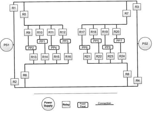
The circuit we want to monitor is composed of four types of devices: generators (also called power supplies), relays, power panels, and wires. By switching relays between passing and blocking states, the system is able to power some set of power panels with some set of generators. A power panel is powered by a power supply if they are connected by a sequence of closed relays. Figure 3-1 displays the structure of

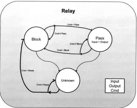
the circuit. Power supplies and relays may receive commands to power on and off, or close and open, respectively, as shown in Figure 3-2. These components have a certain probability to fail and they can be reset.

Power

Supply Connection

Figure 3-1: Redundant Power Distribution System Model The modes of the different components are described as follows.

" A power supply can be in a Powered (output = 1), Not Powered (output = 0),

or Unknown mode.

" A relay can be in a Closed (input = output), Open, or Unknown mode.

" A power panel can be in a Nominal (power = (inputilinput2)) or Unknown

mode. Power panels model all the external devices that are powered by the power distribution system, such as pumps, or A/C systems.

Our model rules out problems of faulty conduction or delivery capacity of wires: perfect wires instantly provide full power when they are connected to a powered gen-erator, and the power state is a boolean value. The circuit has multiple redundancies,

Relay

Figure 3-2: Model of the behavior of a relay

because generators are connected to multiple relays and power panels have two in-puts, so there may be multiple relay switching scenarios that power the same set of power panels with diverse generator configurations. In this model, we exclude the possibility of short-circuit occurrences, supposing that generators are properly pro-tected and grounded. Moreover, each component is always in a well-defined mode,

and we suppose that the mode transitions are synchronous.

The next subsection describes our model for the dynamics of the circuit compo-nents, including when each of them can receive an individual command every time step.

3.4.2

Component Dynamics

We suppose that the different modules of our system evolve synchronously between

different modes, and this evolution is subject to probabilistic transitions. As transi-tions of each component are subject to randomness, we can only estimate the system dynamics through observations of hidden states.

In our model, generators can nominally receive 2 types of commands, switching between the modes Powered and Not Powered. On or Of f commands change the values of the generators' respective outputs at the successive time steps.

Relays are commanded to switch to Pass or Block modes, and a power panel is

considered powered if one of its inputs is fed by a current. However, if a generator, a

relay, or a power panel does not exhibit a nominal behavior, that is, does not switch correctly to the commanded mode, it is in an unknown, off-nominal mode.

It is possible to exit off-nominal modes by sending the Reset command to a given component. The Reset commands revert components to their default mode, which are Not Powered or Block.

3.4.3

Monitoring Problem

The monitoring problem in this example consists of determining the most likely mode configuration of each component, and should a failure happen, it determines which