HAL Id: hal-01896122
https://hal.archives-ouvertes.fr/hal-01896122
Submitted on 16 Oct 2018
HAL is a multi-disciplinary open access
archive for the deposit and dissemination of
sci-entific research documents, whether they are
pub-lished or not. The documents may come from
teaching and research institutions in France or
abroad, or from public or private research centers.
L’archive ouverte pluridisciplinaire HAL, est
destinée au dépôt et à la diffusion de documents
scientifiques de niveau recherche, publiés ou non,
émanant des établissements d’enseignement et de
recherche français ou étrangers, des laboratoires
publics ou privés.
Strong-coupling fixed point instability in a
single-channel S U ( N ) Kondo model
Andres Jerez, M. Lavagna, Damien Bensimon
To cite this version:
Andres Jerez, M. Lavagna, Damien Bensimon. Strong-coupling fixed point instability in a
single-channel S U ( N ) Kondo model. Physical Review B: Condensed Matter and Materials Physics
(1998-2015), American Physical Society, 2003, 68 (9), �10.1103/PhysRevB.68.094410�. �hal-01896122�
Strong-coupling fixed point instability in a single-channel SU
„N… Kondo model
Andre´s Jerez,1 Mireille Lavagna,2,*and Damien Bensimon2,31European Synchrotron Radiation Facility, 6, rue Jules Horowitz, 38043 Grenoble Cedex 9, France 2Commissariat a` l’Energie Atomique, DRFMC /SPSMS, 17, rue des Martyrs, 38054 Grenoble Cedex 9, France
3Department of Applied Physics, University of Tokyo, Bunkyo-Ku, Tokyo 113-8656, Japan
共Received 20 December 2002; revised manuscript received 5 June 2003; published 12 September 2003兲 We study a generalized SU(N) single-impurity Kondo model in which the impurity spin is described by a combination of q Abrikosov fermions and (2S⫺1) Schwinger bosons. Our aim is to describe both the quasi-particlelike excitations and the locally critical modes observed in various physical situations, including non-Fermi-liquid behavior in heavy-fermion systems in the vicinity of a quantum critical point. We carry out an analysis of the strong-coupling fixed point, from which an effective Hamiltonian is derived containing both a charge interaction and a spin coupling between ndnearest-neighbor electrons and the screened impurity. The effective charge interaction is already present in the case of a purely fermionic impurity and it changes from repulsive to attractive at q⫽N/2, due to the q→N⫺q symmetry. The sign of the effective spin coupling determines the stability of the strong-coupling fixed point. Already in the single-channel case and in contrast with either the pure bosonic or the pure fermionic case, the strong-coupling fixed point is unstable against the conduction electron kinetic term in the large-N limit as soon as q⬎N/2. The origin of this change of regime is directly related to the sign of the effective charge interaction.
DOI: 10.1103/PhysRevB.68.094410 PACS number共s兲: 75.20.Hr, 75.30.Mb, 71.10.Hf I. INTRODUCTION
Recent experiments in heavy-fermion compounds have shown the existence of a quantum phase transition from a magnetically disordered to a long-range magnetic ordered phase, driven by change in chemical composition, pressure, or magnetic field.1For an extensive survey of the experimen-tal situation we refer the reader to the review paper of Stewart.2In a very unusual way, the behavior of the system in the disordered phase close to the quantum critical point 共QCP兲 differs from that of a Fermi liquid. For example CeCu6⫺xAux共Refs. 3 and 4兲 and (Ce1⫺xLax)Ru2Si2 共Ref. 5兲
present an antiferromagnetic transition, respectively, at x
C
⫽0.1 and xC⫽0.08. While far from the QCP, the magneti-cally disordered phase is a Fermi liquid with a large effective mass, the temperature dependence of the physical quantities in the disordered phase in the vicinity of the QCP is of non-Fermi-liquid-like type. Typically, in CeCu5.9Au0.1,4the
spe-cific heat C depends on T as C/T⬃⫺ln(T/T0), the magnetic susceptibility as ⬃1⫺␣
冑
T, and the T-dependent part ofthe resistivity as ⌬⬃T instead of C/T⬃⬃Const and ⌬ ⬃T2 as in the Fermi-liquid state. Once a long-range
mag-netic order is set up, the effect of a pressure or of a magmag-netic field is to drive the system back to a magnetically disordered phase with a Fermi-liquid behavior. The same type of behav-ior has been observed in other systems such as YbRh2Si2,
6
CeNi2Ge2,7 CeCu2(Si1⫺xGex)2,8 CeIn3, CePd2Si2,9 and U1⫺xYxPd3.10The associated breakdown of the Fermi-liquid
theory poses fundamental questions about the possible for-mation of novel electronic states of matter with new types of elementary excitations resulting from the presence of strong correlations among electrons.
On the theoretical side, two scenarios are in competition to describe quantum phase transitions: either the itinerant magnetism scenario 共i兲, or more recently proposed, the lo-cally critical picture 共ii兲.
In the former case, 共i兲, the quasiparticles still exist at the QCP and the theory focuses on the study of the low-lying, large-wavelength 共low-, low-q) fluctuations of the order parameter close to the transition. The calculations have been performed within the renormalization-group scheme11–13 or in the self-consistent spin-fluctuation theory,14and have been recently extended15 to the microscopic model which is be-lieved to describe the heavy fermions, the Kondo lattice. In all the cases, they lead to a ⌽4 theory with an effective dimension de f f⫽d⫹z where d is the spatial dimension and z is the dynamic exponent. In the experimental situations, de f f
is above its upper critical value equal to 4, since d is equal to 3 or 2, and z varies from 2 to 3 depending on whether the spin fluctuations are staggered or uniform. Hence the system is described by a Gaussian fixed point with anomalous tem-perature dependence of C/T and a⫽⌬/T but with predic-tions that cannot account for the non-Fermi-liquid behavior observed experimentally.
The second scenario, 共ii兲, has been motivated by the re-cent results obtained by inelastic neutron-scattering experi-ments performed on CeCu5.9Au0.1. The dynamical spin sus-ceptibility
⬙
(q,) near the magnetic instability wave vectorQ has been found to obey an anomalous/T scaling law16,17 as a function of temperature:
⬙
(Q,)⬃T⫺␣g(/T) with an exponent␣ of order 0.75. Moreover, such a and T depen-dence appear to stand over the entire Brillouin zone reveal-ing in the bulk susceptibility too. This fact strongly suggests that the spin dynamics are critical not only at large length scales18,19but also at atomic length scales, contrary to what happens in the traditional itinerant magnetism picture, 共i兲. From these results, one can deduce that local critical modes coexist with large-wavelength fluctuations of the order pa-rameter implying a non-Gaussian fixed point beyond the⌽4 theory.Alternative theories to the spin-fluctuation scheme are needed to describe the local feature of the quantum critical point characterized by the simultaneous disappearance of the
quasiparticles and the formation of local moments. This has been the subject of much interest these last years with the consideration of single-impurity Kondo models including coupling either to soft-gap fermionic bath or to both fermi-onic and bosfermi-onic baths 共for a review, see Ref. 20兲. The former case corresponds to a fermionic bath with a vanishing density of states at the Fermi level21following a power law
(⑀)⬃兩⑀兩r(r⬎0). It is known to display a quantum critical point QCP driven by critical local-moment fluctuations, from a strong-coupling 共SC兲 phase with complete Kondo screen-ing to a local moment 共LM兲 phase.21–23The QCP is charac-terized by nontrivial behavior of the system as, for instance, scaling law for the dynamical spin susceptibility22following
⬙
()⬃g(/T). The second case corresponds to coupling to both fermionic and bosonic baths where bosons represent collective spin excitations 共see Refs. 20 and 19, and refer-ences within兲. As expected, the bosonic excitations become gapless at the QCP and the spectral density follows a power law in. This model shows strong similarities with the soft-gap model mentioned just above with suppression of the Kondo effect due to critical local-moment fluctuations lead-ing to a local-moment phase. Here again recent calculations based on numerical renormalization group 共NRG兲 or dy-namical mean field theory approaches19seem to indicate the existence of scaling law in /T for the dynamical spin sus-ceptibility in the vicinity of the QCP.The other theories developed so far in order to describe the local QCP, are based on the idea of supersymmetry.24 –27 In these theories, the spin is described in a mixed fermionic-bosonic representation. The interest of the supersymmetric approach is to allow to describe the quasiparticles and the local moments on an equal footing through the fermionic and the bosonic part of the spin, respectively. It appears to be specially well indicated in the case of the locally critical scenario in which the magnetic temperature scale TNand the
Fermi scale TK 共the Kondo temperature兲 below which the
quasiparticles die, vanish at the same point,␦C.
An important aspect in the discussion of the breakdown of the Fermi-liquid theory is related to the question of the sta-bility of the SC fixed point. Whereas all the issues presented previously concerning heavy-fermion systems have to do with properties of the lattice, the instability of the SC fixed point can be regarded already by studying the single-impurity problem.
The traditional source of instability in the single-impurity Kondo model is the presence of several channels for the conduction electrons with the existence of two regimes, un-derscreened and overscreened, with very different behaviors as we are about to recall. Indeed we will see that this is not the only possible source of instability of the strong-coupling fixed point. Recent works have shown that more general Kondo impurities of symmetry group SU(N) may also lead to an instability of the SC fixed point already with one chan-nel of conduction electrons.26,27
In order to fix ideas, let us start with the antiferromagnetic single-channel Kondo impurity model. It is well known that within a renormalization group 共RG兲 analysis,28 –30the flow takes the Kondo coupling J all the way to strong coupling.
The weak-coupling  function follows the renormalization group equation
共g兲⫽dgd共⌳兲⌳ ⫽⫺g2, 共1兲 where g⫽0J and0 is the density of states of conduction
electrons. The system flows to a strong coupling fixed point which is stable and the associated behavior of the system is that of a local Fermi liquid.
The situation is rather different when one considers sev-eral channels for the conduction electrons. In the case of a spin S in Kondo interaction with conduction electrons be-longing to K different channels, Blandin and Nozie`res31have shown that the multichannel Kondo model can lead to two very different situations depending on how K compares to 2S. Their calculation corresponds to a second-order pertur-bation theory in the hopping amplitude t of the conduction electrons, around the strong-coupling fixed point. They ana-lyze their results by deriving an effective coupling Je f f
be-tween the spin of the composite formed by the impurity dressed by the conduction electrons in the strong-coupling limit, and the spin of the conduction electron on the neigh-boring sites. They are then able to apply the same RG analy-sis to Je f f as indicated in Eq. 共1兲. In the underscreened re-gime, when K⬍2S, the effective coupling is found to be ferromagnetic and the strong coupling fixed point is stable. In the overscreened regime when K⬎2S, the effective cou-pling is found to be antiferromagnetic and hence the strong-coupling fixed point is unstable. The former K⬍2S regime corresponds to the one-stage Kondo effect with the formation of an effective spin (S⫺1/2) resulting from the screening of the impurity spin by the conduction electrons located on the same site. The system described by the strong-coupling fixed point, behaves as a local Fermi liquid. The instability of the strong-coupling fixed point in the overscreened regime is an indication of the existence of an intermediate coupling fixed point which has been then investigated32–34 by means of other methods. As is well established now, the intermediate coupling fixed point leads to non-Fermi-liquid excitation spectrum with an anomalous residual entropy at zero tem-perature.
It has recently been put forward that other sources of in-stability of the SC fixed point may exist besides the multi-plicity of the conduction electron channels. Recent works26,27 have shown that the presence of a more general Kondo im-purity where the spin symmetry is extended from SU(2) to SU(N), and the representation is given by a L-shaped Young tableau, may also lead to an instability of the SC fixed point already in the one-channel case. In the large N limit, Cole-man et al. 共Refs. 26 and 27兲 have found that the SC fixed point becomes unstable as soon as q共the number of boxes in the Young tableau along the first column兲 is larger than N/2, whatever may be the value of 2S 共the number of boxes in the Young tableau along the first row兲. The consideration of a L-shaped Kondo impurity fits in with the supersymmetry ap-proach that we have evoked before since both spin operators and states can be expressed in terms of bosons and fermions. 共2003兲
At that point, it is worth noting that the supersymmetry theory, or specifically taking into consideration more general L-shaped Kondo impurities, appears to offer valuable in-sights into the two issues raised by the breakdown of the Fermi-liquid theory that we have summarized above, i.e., both the existence of locally critical modes and the question of the instability of the SC fixed point. In the same way as large N expansions may provide insights into real systems even at finite value of the degeneracy, the study of more general impurities may enlighten the understanding of ex-perimental situations with the coexistence of quasiparticles and localized moments that may eventually lead to a phase transition as the coupling to other impurities become domi-nant.
The aim of the paper is to study the L-shaped, single-impurity, single-channel, SU(N) Kondo model. We want to understand how the system behaves, not only as a function of the impurity parameters (2S,q), but also as a function of the number of electrons ndavailable on neighboring sites, that is
to say, of the filling. As long as the bosonic component of spin is of order N, there is a transition around the point where the fermionic component of the impurity is q⫽N/2. At this particular point, the energy shift is, to lowest order in pertur-bation theory around the strong-coupling fixed point, equal to (⫺2t2/J), independently of the impurity parameters, q, S, and N. Our study reveals that the phase diagram of the sys-tem is not accidental, but is due to the relation of the effec-tive dressed impurity in the strong-coupling regime to the conduction electrons in neighboring sites. If q⬍N/2, there is a repulsive effective potential acting on the nearest-neighbor site of the impurity. This potential becomes attractive for q ⬎N/2. This change in behavior happens at the same place where the strong-coupling fixed point becomes unstable. That is, in the repulsive regime the strong-coupling fixed point is stable. However, the attractive regime is not realized as such since the strong-coupling fixed point becomes un-stable for q⬎N/2.
The rest of the paper is organized as follows. In Sec. II, we introduce the model and the main features of the strong-coupling limit, where the electron kinetic term is neglected. In this limit the model is reduced to a single site problem, where the impurity is coupled to nc conduction electrons.
27
We identify the ground state and the energies of the excited states with one more or one less conduction electron, which will play a role in the lowest order in perturbation theory. In Sec. III, we derive the effective Hamiltonian resulting from a second-order perturbation calculation in t around the strong-coupling fixed point. It includes both an effective strong-coupling and an effective interaction between the dressed impurity at site 0 and the conduction electrons on the adjacent site. The sign of the effective spin coupling Je f f directly controls the
stability of the strong coupling fixed point in the sense that
Je f f can be incorporated in turn into the
renormalization-group equations driving the renormalization flow of the sys-tem. When the effective coupling Je f f is ferromagnetic, the
flow takes the system to Je f f⫽0 and the strong-coupling
fixed point turns out to be stable. When the effective cou-pling Je f f is antiferromagnetic, the flow takes the system away from the strong-coupling fixed point to an intermediate
coupling fixed point. The sign of the effective charge inter-action Ue f f informs on the repulsive or attractive effect of
the dressed impurity on the conduction electrons on the ad-jacent site. Section IV contains the discussion of the results. In the large N limit, we show how Je f f is derived from the
energy shift difference between the symmetric and the anti-symmetric configurations, and how the analysis of the nd
dependence of the energy shift provides information on the effective charge interaction Ue f f. When the behavior of the
system is controlled by the strong-coupling fixed point, i.e., when q⬍N/2, the impurity in the ground state tends to repel electrons on neighboring sites. Once q⬎N/2, the repulsion becomes attraction. We show how this feature is already present in the purely fermionic case, and is a consequence of the particle-hole symmetry, q→N⫺q. The fact that there is extra degeneracy in the supersymmetric impurity, due to the bosonic contribution, leads to the instability of the strong-coupling fixed point as soon as q⬎N/2. We finish the section with a short discussion on the behavior of physical quantities in the different regimes.
The appendixes contain the technical details of the calcu-lations, which involve a higher level of complexity than those of Ref. 27, where only the explicit form of the ground state was needed. When nd⬎1, there is more than one
inter-mediate state in some of the virtual processes considered, and we need to use the explicit form of the intermediate states. In Appendix A we outline the construction of three particle states with SU(3) symmetry, as an introduction to the group theoretical formalism used. Explicit expressions for the impurity states and the eigenstates of the model in the strong-coupling limit are derived in Appendix B. We also include a general presentation of the different representations of the spin, either bosonic, fermionic, or L shaped, as con-sidered in the paper. We will show how in the latter case the spin operators and the impurity states are expressed in terms of fermion and boson creation and annihilation operators within two constraints. Appendix C contains a calculation of the energy shift at the strong-coupling fixed point to lowest order in perturbation theory, for the completely antisymmet-ric impurity. Since the ground state is a singlet, there is no splitting of levels. Nevertheless, the behavior of the energy with the filling, nd, on the neighboring site shares many
common features with the problem that we have studied. Finally, we include the details of the calculation of the matrix elements needed in the second-order perturbation theory cal-culation in Appendix D. We also include several sets of SU(N) Clebsch-Gordan coefficients that we had to evaluate explicitely for arbitrary 2S, q, and nd.
II. THE MODEL AND ITS STRONG-COUPLING LIMIT Here we present the model that we study as well as its ground state and elementary excitations in the strong-coupling (J⫽⬁) limit. The results summarized in this sec-tion were already obtained in Refs. 26 and 27. However, technical details such as the explicit form of the eigenstates included in Appendix B, are original.
A. SU„N… single-impurity Kondo model
We consider a generalized, single-impurity, Kondo model with one channel of conduction electrons and a spin symme-try group extended from SU(2) to SU(N). An impurity spin
S is placed at the origin 共site 0). In this paper we will deal
with impurities that can be realized by a combination of bosonic and fermionic operators, and are thus described by a L-shaped representation in the language of Young tableaux,35–37as illustrated in Fig. 1共for details, see Appen-dix B兲.
If 2S and q are the numbers of boxes along the first row and the first column, respectively, the representation is de-noted by 关2S,1q⫺1兴. Its degeneracy38is reported in Table I. The conduction electrons transform under the fundamental representation of SU(N) and can be represented by Young tableaux made out of single boxes. The dimension of the fundamental representation is N, which just means that each electron can be in one of N states of spin.
The Hamiltonian describing the model is written as
H⫽
兺
k,␣ k ck,␣ † ck,␣⫹J兺
A SA兺
␣, c␣ †共0兲 ␣ A c共0兲, 共2兲where ck,†␣ is the creation operator of a conduction electron with momentum k, SU(N) spin index ␣⫽a,b, . . . ,rN,
c␣†(0)⫽1/
冑
NS兺kck,␣†
is the creation operator of a conduction electron at the origin, NS is the number of sites, and ␣A
(A⫽1, . . . ,N2⫺1) are the generators of the SU(N) group in the fundamental representation, with Tr关AB兴⫽␦AB/2. In
the SU(2) case, A⫽A/2, where 兵A其 are the Pauli matri-ces. The conduction electrons interact with the impurity spin
SA(A⫽1, . . . ,N2⫺1), placed at the origin, via Kondo cou-pling, J⬎0. When the impurity is in the fundamental repre-sentation, we recover the Coqblin-Schrieffer model30,39 de-scribing conduction electrons in interaction with an impurity
spin of angular momentum j, (N⫽2 j⫹1), resulting of the combined spin and orbit exchange scattering. In our notation,
a⫽ j, b⫽ j⫺1, . . . ,rN⫽⫺ j.
B. Strong-coupling fixed point
In the strong-coupling limit, the Hamiltonian reduces to the local Kondo interaction term at site 0,
H⫽J
兺
A SA兺
␣, c␣ †共0兲 ␣ A c 共0兲. 共3兲The ground state, 兩GS
典
, is formed by binding the right amount of conduction electrons to the impurity in order to minimize the Kondo energy. Let us denote by Y共Fig. 2兲 the representation of the ncconduction electrons coupled to theimpurity, R that of the free impurity 共Fig. 1兲, and RSC the
representation of one of the strong-coupling states resulting of the direct product R丢Y 共cf. Fig. 3兲 共see Appendix B for
details兲.
When N⫽2, the Kondo energy can be written in terms of conserved quantities JSᠬ•
兺
␣, c␣ †共0兲ᠬ ␣c共0兲 兩GS典
⫽J2关SSC共SSC⫹1兲⫺SR共SR⫹1兲⫺SY共SY⫹1兲兴兩GS典
,where S(S⫹1) is the eigenvalue of the Casimir operator Sˆ2 for N⫽2. The generalization to SU(N) is given by
J
兺
A sA兺
␣, c␣ †共0兲 ␣ A c 共0兲兩GS典
⫽2J关Cˆ2共RSC兲⫺Cˆ2共R兲⫺Cˆ2共Y 兲兴兩GS典
, 共4兲 FIG. 1. Young tableau description of an impurity with mixedsymmetry, 关2S,1q⫺1兴, realized by a combination of fermions and bosons.
TABLE I. Dimension d and eigenvalues of the Casimir operatorC2 for the symmetric, antisymmetric,
L-shaped, and fundamental representations studied in this paper. In the L-shaped case, Q⫽(2S⫹q⫺1) is the total number of boxes in the Young tableau, and Y⬘⫽(q⫺2S) measures the row-column asymmetry.
Symmetric Antisymmetric L shaped Fundamental
关2S兴 关1q兴 关2S,1q⫺1兴 关1兴 d CN2S⫹2S⫺1 CNq
冉
2S 2S⫹q⫺1冊
CN⫹2S⫺1 2S CNq⫺1⫺1 N C2 1 2N 关2S(2S⫹N)(N⫺1)兴 1 2N 关q(N⫺q)(N⫹1)兴 Q 2(N⫺Y⬘⫺Q/N) 1 2N(N 2⫺1)FIG. 2. Young tableau description of nc conduction electrons, localized at the impurity site.
whereC2(Rˆ ) is the quadratic Casimir operator of the
repre-sentation Rˆ , which commutes with all the generators of the group. For a representation given by a Young tableau with mj boxes in the j th row until the row j⫽h⬍N, the eigenvalue C2(兵mj其) of the quadratic Casimir operator is
C2共兵mj其兲⫽ 1 2
冋
Q共N2⫺Q兲 N ⫹j兺
⫽1 h mj共mj⫹1⫺2 j兲册
,where Q⫽兺hj⫽1mj is the total number of boxes.40 Table I
summarizes the expressions of the Casimir eigenvalues for the impurities described in this work and for the conduction electrons, as well as the dimension of their spin representa-tions.
Minimization of the energy, Eq. 共4兲, leads to a ground state with nc⫽(N⫺q) conduction electrons coupled to the
L-shaped Kondo impurity ensuring partial screening. The re-sulting composite at site 0, with energy E0, is made out of
the impurity dressed by the conduction electrons in order to form a singlet along the first column. The associated Young tableau in the strong-coupling regime is given in Fig. 3. Note that the first column of length N can be removed without changing the representation since it is a singlet. When the strong-coupling fixed point is stable, this corresponds to a one-stage Kondo effect in which the impurity is screened by the conduction electrons to form a bosonic (S⫺1/2) impurity.
C. Ground state
Let us now write the expression of the fundamental state associated with this strong-coupling fixed point. The ground state is degenerate. The states in the multiplet transform as a completely symmetric representation of SU(N), described by a Young tableau with (2S⫺1) boxes, denoted by 关2S ⫺1兴 共Fig. 3兲. We choose a realization of the impurity in terms of 2S bosonic operators and (q⫺1) fermionic opera-tors, which happens to be more convenient. We could have constructed impurity states with the same SU(N) symmetry using (2S⫺1) bosons and q fermions 共see Appendix B兲. We would like to emphasize that all the results that we establish in this paper are independent of the operator representation which we choose to work with. The highest weight state is then written as 兩GS
典
兵a其aa [2S⫺1]⫽ 1冑
共2S⫺1兲!共ba †兲2S⫺1兩⌬典
共5兲 with 兩⌬典
⬅1␥A冋
bi 1 †冉
兿
␣⫽i2 iq f␣†冊冉
兿
⫽iq⫹1 iN c†冊
册
兩0典
, 共6兲 ␥⬅冑
共2S⫹N⫺1兲CN⫺1 q⫺1 .Here,兩⌬
典
transforms itself as a SU(N) singlet and it will be annihilated by any of the raising and lowering operators,T⫾兩⌬
典
⫽U⫾兩⌬典
⫽•••⫽0. This ‘‘state’’ would describe thestrong-coupling ground state for a purely fermionic impurity. D. Excited states
There are two types of excited states in the strong-coupling regime. Either the degenerate ground state acquires an additional conduction electron at the impurity site 兩GS ⫹1
典
, or it loses one conduction electron, 兩GS⫺1典
. In the former case 兩GS⫹1典
the spin of the additional conduction electron can be either symmetrically or antisymmetrically correlated with the spin of the impurity as schematized in Fig. 4.In the limiting case of SU(2) spin, these two configura-tions correspond to a spin of the conduction electron that is either parallel or antiparallel to the impurity spin. In the gen-eral SU(N) case, we will keep on speaking of symmetric and antisymmetric configurations, respectively.
States with one less electron will be denoted by 兩GS ⫺1
典
and are represented by the Young tableau in Fig. 5. Let us denote by ⌬E1S⫽E1S⫺E0, ⌬E1A⫽E 1 A⫺E
0, and⌬E2⫽E2
⫺E0 the energy differences, with respect to the ground-state
energy, associated with these three excited states兩GS⫹1
典
S, 兩GS⫹1典
A, and 兩GS⫺1典
. Using the same Casimirologymethod as presented at the beginning of this section for the determination of the ground-state energy, we have summa-rized our results in Table II, respectively, for arbitrary N and in the large-N limit with (2S⫹q⫺1)/N finite. One can
FIG. 3. Young tableau description of the formation of the strong coupling ground state. We denote the presence of conduction elec-trons at site 0 by c. Notice that the first column in the Young tableau for RSCis a singlet and can be removed.
FIG. 4. Excited states 兩GS⫹1典S and 兩GS⫹1典A with an addi-tional conduction electron nc⫽(N⫺q⫹1), respectively, in the symmetric and antisymmetric configurations.
FIG. 5. Excited state兩GS⫺1典with one less conduction electron nc⫽(N⫺q⫺1).
check that the results in Table II coincide with Eqs.共25兲 and 共26兲 of Ref. 27, within a N/2 factor stemming from a differ-ent definition of the Kondo coupling J关cf. Eq. 共1兲of Ref. 27兴 and of the Casimir关cf. Eq. 共17兲 of Ref. 27兴, and a change in the notations n*f⫽q and nb⫽2S.
Notice that the excitation energies⌬E1 A
and⌬E2, in the
large N limit, are independent of S, and related by the
particle-hole transformation q→N⫺q, characteristic of the
problem with a purely antisymmetric impurity, 2S⫽1 共see Appendix C兲.
III. STABILITY OF THE STRONG-COUPLING FIXED POINT
We have identified the strong-coupling fixed point in the preceding section. For J→⬁, the lowest energy state corre-sponds to nc⫽(N⫺q) electrons partially screening the
im-purity at the origin, and isolated from the rest of the bulk which may be described by a chain of electrons, for conve-nience.
In order to better understand the low-energy physics of the system, we can perform a strong-coupling analysis con-sidering a finite Kondo coupling and allowing virtual hop-ping from and to the impurity site. These processes generate interactions between the composite at site 0 and the conduc-tion electrons on neighboring sites, which can be treated as perturbations of the strong-coupling fixed point. Applying an analysis similar to that of Nozie`res and Blandin31to the na-ture of the excitations, we can argue whether or not the strong-coupling fixed point remains stable once virtual hop-ping is allowed.
We consider a system with an additional site next to the dressed impurity, filled with nd electrons. The ground state
consists of two multiplets, with different symmetry proper-ties. Once the hopping is turned on, the degeneracy is lifted, and each multiplet acquires a different energy shift denoted by ⌬ES and ⌬EA, respectively 共see Fig. 6兲. We can
repro-duce this spectrum by considering an effective coupling be-tween the spin of the dressed spin at site 0, and the spin of the nd electrons on site 1. If ES lies共above兲 below EA, the
effective coupling is 共antiferromagnetic兲 ferromagnetic. Thus, if the coupling between the effective spin at the impurity site and that of the electrons on site 1 is ferromag-netic we know, from the scaling analysis at weak coupling, that the perturbation is irrelevant, and the low-energy physics
is described by the strong-coupling fixed point. That is, an underscreened, completely symmetric, effective impurity weakly coupled to a gas of free electrons with a phase shift indicating that there are already (N⫺q) electrons screening the original impurity. In the completely antisymmetric case (2S⫽1), the phase shift corresponds to the unitary limit,␦ ⫽/2, for SU(2), and is a function41 of q/N for SU(N), reaching the unitary limit for q⫽N/2.
If, on the contrary, the effective coupling is antiferromag-netic, the perturbation is relevant, this strong-coupling fixed point is unstable and it does not describe the low-energy physics of the model.
In this section we explicitely calculate the effects of hop-ping on the strong-coupling fixed point to the lowest order in perturbation theory, that is, second order in t. We will con-sider the case with an arbitrary number nd of conduction
electrons in site 1 generalizing the case nd⫽1 considered in
Ref. 27. This will allow us to understand the origin of the instability of the strong-coupling fixed point.
Before switching on the hopping term, let us consider
ground states of the form 兩GS,nd
典
⫽兺兩GS典
0兩nd典
1, with ndFIG. 6. Second-order perturbation theory energy shift of the strong-coupling ground state in the cases of a ferromagnetic共a兲 and antiferromagnetic共b兲 effective coupling.
TABLE II. Strong-coupling excitation energies, ⌬E1
S , ⌬E1
A
, and ⌬E2, in the case of an L-shaped
impurity, measured with respect to the ground state, of the states with one more conduction electron on site 0, coupled symmetrically and antisymmetrically, respectively, to the dressed impurity on site 0, and of the state with one less electron.
⌬E1 S ⌬E 1 A ⌬E 2 Arbitrary N J 2(2S⫹N⫺q⫺Q/N) J 2(N⫺q⫺Q/N) J 2(q⫹Q/N) Large N limit (Q/N finite兲 J 2(N⫺q⫹2S) J 2(N⫺q) J 2q 共2003兲
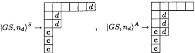
electrons on site 1. According to the SU(N) symmetry there are two possible configurations, depending on whether the nd electrons are coupled symmetrically or antisymmetrically to the composite on site 0. This corresponds to the Clebsch-Gordan series 关2S⫺1兴丢关nd兴→关2S,1nd⫺1兴丣关2S⫺1,1nd兴.
We denote the states by 兩GS,nd
典
S, and 兩GS,nd典
A,respec-tively共Fig. 7兲.
The SU(N) symmetry is preserved by the hopping. That means that the perturbation will shift the energies of
兩GS,nd
典
Sand兩GS,nd典
Aseparately, without mixing the states.We will thus denote the shifts by ⌬E0S and ⌬E0A, respec-tively.
The hopping term is of the form
Hh⫽H1⫹H2⫽t
兺
␣ c␣ †d ␣⫹t兺
␣ d␣ †c ␣, 共H1兲†⫽H2,where d␣† creates an electron on site 1. We can distinguish two types of processes, corresponding to different intermedi-ate stintermedi-ates.27 The first type, which we denote process 1, cor-responds to an electron hopping from site 1 into site 0 first, probing excited states兩GS⫹1
典
S,A, and then hopping back to site 1. The indices S,A correspond to the two possible inter-mediate states depending on whether the conduction electron that hops to site 0 is symmetrically or antisymmetrically cor-related with the dressed impurity as we will see in detail below. The contribution of the process 1 to the energy shift is the following: t2兺
␣,兺
i具
GS,nd兩d†c兩GS⫹1,nd⫺1典
ii具
GS⫹1,nd⫺1兩c␣†d␣兩GS,nd典
共E0⫺E1 i兲 ,with i⫽S,A 共see Appendix B兲.
In process 2, the electron hops from site 0 to site 1 first and then back to site 0, probing兩GS⫺1
典
, leading to a contribution to the energy shift of the formt2
兺
␣,
具
GS,nd兩c†d兩GS⫺1,nd⫹1典具
GS⫺1,nd⫹1兩d␣†c␣兩GS,nd典
共E0⫺E2兲
.
Hence, the energy shifts for the symmetric and antisymmet-ric configurations are, respectively,
⌬E0 S⫽ M1 S E0⫺E1 S⫹ M1S E0⫺E1 A⫹ M2S E0⫺E2 , 共7兲 ⌬E0 A⫽ M1 A E0⫺E1 A⫹ M2A E0⫺E2, 共8兲
where the expressions in the denominators, (E0⫺E1 S ) ⫽⫺⌬E1 S, (E 0⫺E1 A)⫽⫺⌬E 1 A, and (E
0⫺E2)⫽⫺⌬E2
mea-suring the energy of the excited states compared to the en-ergy of the ground state are given in Table II. The matrix elements M will be introduced below as we will study the contribution of each process. The energy difference between the two states,
⌬E0 S⫺⌬E 0 A⫽ M1 S E0⫺E1 S⫹ M1S⫺M1A E0⫺E1 A ⫹ M2S⫺M2A E0⫺E2 , 共9兲
determines the sign of the effective interaction and the sta-bility of the strong-coupling fixed point. If we compare Eq.
共9兲 to the nd⫽1 result in Ref. 27, we see that there is an
additional contribution M¯ 1S, present for nd⬎1.
A. Process 1: Symmetric configuration
We consider first the case where the nd electrons in the
site 1 are coupled to the site-0 state in the most symmetric configuration. In the shorthand notation that we use for the Young tableaux, it corresponds to the state 关2S⫺1兴丢关1nd兴 →关2S,1nd⫺1兴. Here, as opposed27 to the case n
d⫽1, the
Hamiltonian transforms the ground state 兩GS,nd
典
S⫽共da†
db†•••du†兲兩GS
典
, 共10兲 into a linear combination of two excited states: 兩GS⫹1,nd⫺1
典
S, with energy ES, and 兩GS⫹1,nd⫺1
典
S, with energyEA depending on whether the additional conduction electron
in site 0 is coupled symmetrically or antisymmetrically to the dressed impurity. The state obtained by acting with c†d on the ground state defined by Eq. 共10兲 has to be computed explicitely, and the result written as a linear combination of the excited states, Fig. 8. The latter are obtained by coupling the site-0 states with (nd⫺1) conduction electrons on site 1. FIG. 7. Strong-coupling ground states in the presence of nd
conduction electrons on site 1 coupled either symmetrically or an-tisymmetrically to the dressed impurity on site 0.
The explicit expressions for these states are given in Appen-dix D, and they lead to the result
冉
兺
c†d冊
兩GS,nd典
S ⫽⍀冑
2S⫹nd⫺1 2S 兩GS⫹1,nd⫺1典
S ⫹⌳冑
nd⫺1冑
2S⫺1 2S 兩GS⫹1,nd⫺1典
S, 共11兲where the normalization coefficients,27 ⍀ ⫽
冑
(2S⫹q⫺1)/(2S⫹N⫺1) and ⌳⫽冑
(q⫺1)/(N⫺1) are independent of nd, as we are considering hopping of a singleelectron. From here, we obtain the following matrix ele-ments: M1S⫽兩S
具
GS⫹1,nd⫺1兩H1兩GS,nd典
S兩2 ⫽t2冉
2S⫹nd⫺1 2S冊冉
2S⫹q⫺1 2S⫹N⫺1冊
, 共12兲 M1 S⫽兩S具
GS⫹1,n d⫺1兩H1兩GS,nd典
S兩2 ⫽t2共n d⫺1兲冉
2S⫺1 2S冊冉
q⫺1 N⫺1冊
. 共13兲We see right away that M1S is proportional to (nd⫺1), and
vanishes for nd⫽1, whereas M1S depends noticeably on nd only for 2SⰆnd⬍N.
B. Process 1: Antisymmetric configuration
Next, we consider the case where the electrons on site 1 are coupled to the effective spin on site 0 according to 关2S ⫺1兴丢关1nd兴→关2S⫺1,1nd兴. In the preceding section it was
easy to write the strong-coupling ground state by just putting together the effective spin and the nd electrons in the highest
weight state possible, to obtain Eq. 共10兲. Here we have to work out the necessary SU(N) Clebsch-Gordan coefficients. We present some of these coefficients in Table VII of Appen-dix D. The explicit form of the ground state is
兩GS,nd
典
abc . . .v A ⫽ 1冑
2S⫹nd⫺1冋
冑
2S⫺1冉
i兿
⫽2 nd⫹1 dy i †冊
兩GS典
aa ⫹兺
j⫽2 nd⫹1 共⫺1兲j⫺1冉
兿
i⫽1,i⫽ j nd⫹1 dy i †冊
兩GS典
ayj册
, 共14兲 in the notation y1⫽a. As in the nd⫽1 case, the hoppingterm transforms the state defined by Eq. 共14兲 into a state proportional to a given strong-coupling excited state共Fig. 9兲. In order to obtain the corresponding matrix element, we have computed explicitly
冉
兺
c†d冊
兩GS,nd典
A ⬀兩GS⫹1,nd⫺1典
A,and then we have normalized the resulting state. The details can be found in Appendix D. We have
冉
兺
c†d冊
兩GS,nd典
A⫽⌳冑
nd兩GS⫹1,nd⫺1典
A,and the matrix element
M1A⫽兩A
具
GS⫹1,nd⫺1兩H1兩GS,nd典
A兩2⫽t2nd冉
q⫺1 N⫺1冊
.共15兲 Notice the dependence on nd, and the fact that the matrix
element does not depend on 2S. Combining together M1Sand
M1A as it appears in Eq. 共9兲, we have
M1S⫺M1A⫽⫺t2
冉
2S⫹nd⫺12S
冊冉
q⫺1
N⫺1
冊
. 共16兲This is a term with the same nd dependence as M1S but with the opposite sign.
C. Process 2: The trick
Both in the symmetric and antisymmetric configurations in process 2 there is a one-to-one correspondence between the state obtained by the action of H2, and the excited state
with the same symmetry27 共Fig. 10兲. The evaluation of the remaining matrix elements, M2S and M2A, associated with process 2 is simplified by using the following trick connect-ing the matrix elements of processes 1 and 2, respectively. On the one hand, we have in the process 1,
FIG. 8. When nd conduction electrons are coupled symmetri-cally to the dressed impurity at the origin, the term c†d, acting on the ground state, generates a linear combination of two excited states with an additional conduction electron at the origin.
FIG. 9. When nd conduction electrons are coupled antisym-metrically to the dressed impurity at the origin, the term c†d, acting on the ground state, generates state proportional to a given excited state, with additional conduction electron at the origin.
M1S⫹M1S⫽t2
兺
S ⬘具
GS,nd兩d⬘ † c⬘c†d兩GS,nd典
S ⫽t2兺
S ⬘具
d⬘ † 共␦⬘⫺c†c⬘兲d典
S ⫽t2兺
S 具
d †d 典
S⫺␦MS,where ␦MS⫽t2兺⬘S
具
c†d†⬘dc⬘典
S and the expectation value S具典
S should be considered over the ground state, 兩GS,nd典
S. On the other hand, the following property holdsfor the matrix elements of process 2
M2S⫽t2
兺
S ⬘具
GS,nd兩c⬘ † d⬘d†c兩GS,nd典
S ⫽t2兺
S⬘具
c ⬘ † 共␦⬘⫺d†d⬘兲c典
S ⫽t2兺
S 具
c † c典
S⫺␦MS,where in the last line, we have exchanged the dummy vari-ablesand
⬘
. The same relation exists for the antisymmet-ric configuration 共with expectation values taken on 兩GS,nd典
A) M1A⫽t2兺
A 具
d †d 典
A⫺␦MA, M2A⫽t2兺
A 具
c †c 典
A⫺␦MA.Thus, using the trick, we obtain
M2S⫽t2共nc⫺nd兲⫹共M1 S⫹M 1 S兲 ⫽t2共N⫺n d兲
冉
N⫺q N⫺1冊冉
2S⫹N⫺2 2S⫹N⫺1冊
, 共17兲 M2A⫽t2共nc⫺nd兲⫹M1 A⫽t2关N⫺共n d⫹1兲兴冉
N⫺q N⫺1冊
, 共18兲 M2S⫺M2A⫽M1S⫹MS1⫺M1A⫽t2冉
2S⫹nd⫺1 2S⫹N⫺1冊冉
N⫺q N⫺1冊
. 共19兲 IV. DISCUSSIONHaving computed the different matrix elements in the pre-ceding section, we are now in the position of deriving the expressions of the energy shifts ⌬E0S and⌬E0A of the sym-metric and antisymsym-metric configurations, respectively, within the second-order perturbation theory in the hopping term. We propose to transcribe the results in terms of an effective Hamiltonian describing the charge and spin interactions be-tween the dressed impurity at site 0, and the conduction elec-trons in amount nd at site 1. We will then discuss the
impli-cations of the derived effective Hamiltonian on the behavior of the system.
共i兲 The sign of the effective coupling—ferromagnetic ver-sus antiferromagnetic—controlling the stability of the strong-coupling fixed point, determines the onset of two dif-ferent regimes. When q⬍N/2, the effective coupling is found to be ferromagnetic, the perturbation is proved to be irrelevant by use of scaling arguments 关cf. Eq. 共1兲兴, and the strong-coupling fixed point is stable. When q⬎N/2, on the contrary, the effective coupling is found to be antiferromag-netic, the perturbation becomes relevant, and the strong-coupling fixed point is unstable.
共ii兲 There is an effective charge interaction at site 1, in-duced by the virtual hopping of electrons between the impu-rity site and its nearest-neighbor site. The change in the na-ture of this interaction—from repulsive to attractive—is found to happen at the same place where the strong-coupling fixed point becomes unstable. On the one hand, in the regime when the strong-coupling fixed point is stable q⬍N/2, the interaction is repulsive. On the other hand, in the regime q ⬎N/2, the interaction is attractive. However, we emphasize the point that this attraction is never realized as such since the strong-coupling fixed point is then unstable.
Even though the charge interaction remains a weak per-turbation of the full system, its study allows us to better understand the physical properties of the model and the onset of instability of the strong-coupling fixed point at a particular value of q. Indeed, this charge interaction is already present in the case of an antisymmetric impurity, as we will show below. There, the low-energy physics is controlled by the strong-coupling fixed point for all values of q. Nevertheless, there is a change in the sign of the effective charge interac-tion at q⫽N/2, a consequence of the q→N⫺q symmetry in the antisymmetric case. The fact that the coupling Ue f fis the
same共in the large N limit兲 for the general L-shaped impurity as for the completely antisymmetric case, indicates that the properties observed in the former case are linked to the q →N⫺q transformation of the fermionic component of the impurity.
FIG. 10. The term d†c, acting on the ground state with nd electrons on site 1, coupled symmetrically共a兲 or antisymmetrically 共b兲 to the impurity. The result is a state proportional to an excited state with one less electron at the impurity site, coupled to (nd ⫹1) electrons symmetrically 共a兲 or antisymmetrically 共b兲.
A. Energy shifts⌬E0 S
and⌬E0 A
Incorporating the expressions of the matrix elements, Eqs. 共12兲, 共16兲, and 共19兲, and those of the excitation energies 共Table II兲 into Eqs. 共8兲 and 共9兲, one finds
⌬E0 A⫽⫺
冉
2t 2 J冊冋冉
nd N⫺1冊冉
q⫺1 N⫺q⫺Q/N冊
⫹冉
1⫺ nd N⫺1冊冉
N⫺q q⫹Q/N冊册
, 共20兲 ⌬E0 S⫺⌬E 0 A ⫽⫺共2S⫹nd⫺1兲冉
2t2 J冊
⫻再
2S⫹q⫺1 2S共2S⫹N⫺1兲关2S⫹N⫺q⫺共2S⫹q⫺1兲/N兴 ⫹共N⫺1兲共2S⫹N⫺1兲关q⫹共2S⫹q⫺1兲/N兴N⫺q ⫺ q⫺1 2S共N⫺1兲关N⫺q⫺共2S⫹q⫺1兲/N兴冎
. 共21兲 The dependence of (⌬E0S⫺⌬E0A) on (2S⫹nd⫺1) islin-ear and applin-ears factored out. As 2S increases, the energy difference (⌬E0S⫺⌬E0A) becomes smaller. Moreover, the ef-fect of nd on (⌬E0
S⫺⌬E
0 A
) is weak as long as ndⰆ2S.
Until now, we have presented results for arbitrary N. In the rest of the paper, we will frequently consider the large-N limit taking 2S/N and q/N finite. To leading order in 1/N, we can write ⌬E0 A⫽⫺2t 2 J
冋冉
N⫺q q冊
⫺冉
nd N冊冉
N共N⫺2q兲 q共N⫺q兲冊册
, 共22兲 ⌬E0 S⫺⌬E 0 A⫽⫺2t 2 JN冉
2S⫹nd⫺1 2S⫹N⫺q冊冉
N共N⫺2q兲 q共N⫺q兲冊
. 共23兲The energy difference (⌬E0S⫺⌬E0A) is O(1/N), and both energy levels,⌬E0Sand⌬E0A, have the same leading term in
O(1) which is almost independent of 2S. The only
depen-dence in 2S appears in the difference (⌬E0S⫺⌬E0A). B. Effective Hamiltonian
The energy shifts⌬E0 S
and⌬E0 A
can be reproduced from the following effective Hamiltonian, to within an additive constant term C to be defined later on,
He f f⫽Ue f f nd⫹Je f fS0 [2S⫺1]•S
1 [1nd],
where Ue f f and Je f f are the effective charge and spin inter-actions, respectively, between the dressed impurity at site 0 in the strong-coupling limit and the conduction electrons at site 1. In the notations which are used, S0[2S⫺1] and S1[1nd]
represent the corresponding spin operators in the representa-tions关2S⫺1兴 and 关1nd兴, respectively. The spectrum consists
of two multiplets, according to the Clebsh-Gordan series 关2S⫺1兴丢关1nd兴→关2S,1nd⫺1兴S
丣关2S⫺1,1nd兴A, in which the
superindices S and A indicate the symmetric and antisym-metric states, respectively. The energies shifts induced by
He f f can be calculated as before with the aid of Casimir
operators, Eq.共4兲, and we get ⌬E[2S,1nd⫺1] S ⫺⌬E [2S⫺1,1nd] A ⫽Je f f 2 兵C2共关2S,1 nd⫺1兴兲⫺C 2共关2S⫺1,1nd兴兲其 ⫽⫺Je f f 4 共2S⫹nd⫺1兲关Y
⬘
[2S,1nd⫺1]⫺Y⬘
[2S⫺1,1nd]兴 ⫽Je f f 2 共2S⫹nd⫺1兲,where we have used the results of Table I. Since both states have Young tableaux with the same number of boxes, Qe f f
⫽2S⫹nd⫺1, the energy difference depends only on the
sec-ond constraint 共B7兲, Yˆe f f⫽Qe f fY
⬘
共see Appendix B兲. As aconsequence, the dependence on (2S⫹nd⫺1) is factored
out exactly as in Eq.共21兲 and we get by identification
Je f f⫽⫺
冉
4t2 J冊
⫻再
2S⫹q⫺1 2S共2S⫹N⫺1兲关2S⫹N⫺q⫺共2S⫹q⫺1兲/N兴 ⫹共N⫺1兲关2S⫹N⫺1兲共q⫹共2S⫹q⫺1兲/N兴N⫺q ⫺2S共N⫺1兲关N⫺q⫺共2S⫹q⫺1兲/N兴q⫺1冎
, 共24兲 Ue f f⫽2t 2 J 1 N⫺1冉
N⫺q q⫹Q/N ⫺ q⫺1 N⫺q⫺Q/N冊
共25兲with the additive constant term C equal to (⫺2t2/J)(N ⫺q)/(q⫹Q/N).
In the large-N limit with 2S/N and q/N finite, we have
Je f f⫽⫺ 4t2 J 共N⫺2q兲 q共N⫺q兲 1 共2S⫹N⫺q兲, 共26兲 Ue f f⫽2t 2 J 共N⫺2q兲 q共N⫺q兲 共27兲
with C equal to (⫺2t2/J)(N⫺q)/q. Note that Je f f is
O(1/N2) and depends of 2S, while Ue f f is O(1/N) and
in-dependent of 2S. Furthermore, Ue f fis repulsive when Je f f is
ferromagnetic, and attractive when Je f f is antiferromagnetic.
C. Sign of the effective coupling and stability of the strong-coupling fixed point
In Fig. 11 we plot Je f fin the large-N limit as a function of
q/N, for different values of 2S. The effective coupling Je f f
changes of sign at q⫽N/2 as can be seen by inspection of the numerator of the right-hand side of Eq.共26兲. Notice that the value of Je f f is independent of the number of conduction
electrons nd on site 1 and coincides with the result obtained in Ref. 27 for the case nd⫽1. This is due to the cancellation
of the (2S⫹nd⫺1) factor in (⌬E0
S⫺⌬E
0 A
) that we have mentioned above.
The effective coupling remains ferromagnetic as long as
q⬍N/2 corresponding to the situation E0S⬍E0A. We can then use the same scaling argument for Je f f that we used for J in
the weak coupling regime. Incorporating the value of the effective coupling in the renormalization-group equation关cf. Eq.共1兲兴, one can prove the perturbation Je f f to be irrelevant
and the strong-coupling fixed point to be stable. The low-energy physics corresponds then to a system of free electrons that are weakly coupled to an effective impurity spin.
When q⬎N/2, on the contrary, E0A⬍E0S, the effective coupling is found to be antiferromagnetic, Je f f grows in the
renormalization process, and the strong-coupling fixed point (J⫽⬁) is unstable.
The case q⫽N/2 requires particular attention, since the leading contribution to Je f fvanishes. Taking into account the whole expression for the effective coupling, we find that the strong-coupling fixed point for an impurity with q⫽N/2 is stable as long as the bosonic parameter S is smaller than the critical value
S*⫽1
4
冉
N冑
2NN⫺1⫺共N⫺2兲
冊
.In the large-N limit we have
S*⫽
冉
冑
2⫺1 4冊
N⫹ 4⫹冑
2 8 ⫹O共1/N兲⬃ N 10. 共28兲The strong-coupling fixed point at q⫽N/2 becomes unstable already at moderately large values of S. The corresponding phase diagram of the model in the large-N limit, as a func-tion of the impurity parameters, 2S/N and q/N is reported in Fig. 12.
D. Sign of the effective charge interaction
In Fig. 13 we report the dependance of Ue f f on q/N, in
the large N limit. By comparisons of Eqs.共26兲 and 共27兲, one can see that the change of sign of the effective interaction
Ue f f is directly connected to the change of sign of the
effec-tive coupling Je f f 共see also Fig. 11兲. This result has the
im-mediate following physical consequence. In the former re-gime, q⬍N/2, where the strong-coupling fixed point is stable, the effective interaction Ue f f⬎0 is repulsive, and the lowest energy expressed in Eq.共22兲 is obtained for nd⫽1. In FIG. 11. Effective coupling Je f f as a function of q/N, for
dif-ferent values of 2S, in the large-N limit.
FIG. 12. Phase diagram of the model共large N, 2S/N finite兲, as a function of the impurity parameters, 2S/N and q/N. As soon as q⬎N/2 the strong-coupling fixed point becomes unstable. For q ⫽N/2, the strong-coupling fixed point remains stable only for mod-erate values of 2S/N 共short line ending in a point兲.
FIG. 13. Effective charge interaction Ue f fas a function of q/N, in the large-N limit.
the latter regime, q⬎N/2, the effective interaction Ue f f⬎0
is attractive, and the energy is minimized for nd⫽(N⫺1). We have plotted ⌬E0A in Fig. 14. The shaded region corre-sponds to the possible values of⌬E0A for the whole range of
nd, bounded by the limiting cases, nd⫽1 and nd⫽(N⫺1).
Note that at q⫽N/2, ⌬E0A(q⫽N/2)⫽⫺2t2/J for any value of nd.
As has been noted before, ⌬E0 A
is independent of 2S. Therefore,⌬E0A coincides with the energy shift for a fermi-onic impurity 共completely antisymmetric representation兲 as is checked in Appendix C. When the impurity is fermionic, there is no degeneracy of the strong-coupling fixed point, which is always stable, and the lowest-order perturbation theory just shifts the ground-state energy. Nevertheless, there are two regimes, repulsive and attractive, depending on the value of q, and characterized by the value of nd that mini-mizes the energy. This behavior is a consequence of the
particle-hole symmetry in the fermionic case, given by the
transformations q→(N⫺q) and nd→(N⫺nd)共cf. Appendix C兲. The behavior of a fermionic impurity with q is the same as in the case (N⫺q), if we reinterpret the electrons as holes and the impurity as made out of holes. Therefore, if nd⫽1
minimizes the energy for q⬍N/2 共electron repulsion兲, then the energy for a hole impurity, made out of (N⫺q) fermions, is minimized by the state that repels the holes, (N⫺nd)⫽1,
implying an attraction of electrons, nd⫽(N⫺1). This behav-ior is shown in Fig. 15.
The addition of a bosonic component to the impurity, leading to the formation of a row in the L-shaped Young tableau representing the impurity, breaks this particle-hole symmetry. Whereas the two regimes described above are still
present, due to the fermionic component, the degeneracy of the states due to the bosonic component leads to the instabil-ity of the strong-coupling fixed point at the same point as where the the dressed impurity starts attracting the conduc-tion electrons on site 1.
E. Physical properties of the model
We finish by making some remarks on the physical prop-erties of the model in the different regimes. As is common to all models with an antiferromagnetic Kondo coupling, there will be a crossover from weak coupling above a given Kondo scale TK to a low-energy regime. When the
strong-coupling fixed point is stable, we should expect for TⰆTKa
weak coupling of the effective impurity at site 0 with the rest of the electrons. The physical properties at low temperature are controlled by the degeneracy of the effective impurity,
d(关2S⫺1兴)⫽CNN⫹2S⫺2⫺1 . Thus, we should expect a residual entropy Si⬃lnCNN⫹2S⫺2⫺1 and a Curie susceptibility, i
⬃CN⫹2S⫺2
N⫺1
/T, with logarithmic corrections.41,42This is the result that we would expect for a purely symmetric impurity. The difference with respect to the case at hand is that in the L-shaped impurity model only (N⫺q) electrons are allowed at the origin, instead of (N⫺1). Thus, we would expect to find different results for quantities that involve the scattering phase shift of electrons off the effective impurity. Consider, for instance, the 2S⫽1 case. The phase shift␦, of the con-duction electrons scattered off the impurity site, characterizes the impurity contribution to the resistivity i. At zero tem-perature and magnetic field, we have30
i⬀sin2␦. 共29兲
The phase shift for antisymmetric impurities in SU(N) was computed in Ref. 41. In the completely screened case it reads
e2i␦⫽⫺e⫺i(1⫺2q/N). 共30兲
If we choose the phase shift so that兩␦兩⬍/2, we have
␦⫽
冦
冉
Nq冊
, q⬍N/2⫺
冉
N⫺qN冊
, q⬎N/2.共31兲
FIG. 14. Leading-order term in the energy shift,⌬E0
A⬃⌬E
0
S , as a function of q/N, for 1⬍nd⬍(N⫺1) 共shaded region兲, and in the limiting cases nd⫽1 共dashed line兲 and nd⫽(N⫺1) 共straight line兲. Notice that the value at q/N⫽1/2 is equal to ⫺2t2/J, for any nd. Note that for q/N⬍0.5 the energy is minimized for nd⫽1, while for q/N⬎0.5 the minimization is obtained for nd⫽(N⫺1).
FIG. 15. Strong-coupling ground-state configurations in the fer-mionic case, where only hopping to the nearest-neighbor site has been included. When q⬎N/2, the impurity site attracts N⫺1 con-duction electrons.
The unitary limit, 兩␦兩⫽/2 is reached in the particle-hole symmetric case, q⫽N/2. We see that this corresponds to the point where⌬Efis independent of nd, indicating the change
from the attractive to the repulsive regime.
In the q⬎N/2 regime, it is reasonable to think that there would be a magnetic contribution to the entropy, and a Curie-like contribution to the susceptibility, since the impu-rity remains unscreened. This behavior is different from that of the multichannel Kondo model, which is characterized by an intermediate coupling fixed point where the impurity magnetic degrees of freedom are completely quenched.43 It is in the scattering properties that we might be able to see the anomalous features of this new fixed point more clearly.
V. CONCLUSIONS
In this paper, we have studied the SU(N), single-channel Kondo model, with a general impurity spin, involving both bosonic and fermionic degrees of freedom 共corresponding, respectively, to the horizontal and vertical directions in a L-shaped Young tableau兲. This model shows a transition be-tween two different regimes when the amount of fermionic degrees of freedom, q, becomes larger than N/2, in the
large-N limit. The strong-coupling fixed point studied here
de-scribes the low-energy physics of the model when q⬍N/2, and it becomes unstable for q⬎N/2. We have identified the origin of this instability as related to the change, from repul-sive to attractive, of the effective interaction between the dressed impurity and the conduction electrons in the neigh-boring sites. This change is already present in the purely fermionic case, where it happens at the particle-hole symme-try point, q⫽N/2. The only role of the bosonic degrees of freedom of the impurity is to allow for a degeneracy of the strong-coupling fixed point, which is lifted by hopping, lead-ing to an effective spin coupllead-ing Je f f. The properties of this
coupling, as well as the effective charge coupling, are then controlled by the fermionic component of the impurity.
We have followed a systematic approach in order to ob-tain the explicit form of the states needed for our calcula-tions. As a result, our work can be used as the starting point for the study of richer systems, such as the multichannel case.
Obviously, the interesting open problem now is to fully understand the physics in the q⬎N/2 regime. This issue might have important future applications for the lattice prob-lem, with potential consequences for the understanding of non-Fermi-liquid behavior observed in heavy-fermion sys-tems. In order to gain some insight it would be desirable to carry out a nonperturbative study, either using NRG or Bethe ansatz techniques. Here, we would like to point out some of the limitations of these methods when applied to the model under consideration. The effects described in our work ap-pear for N⬎5. That is, each lattice site can be filled with up to five electrons. Furthermore, the simplest impurity that dis-plays an intermediate fixed point corresponds to a multiplet with 45 elements. Such a large Hilbert space limits the per-formance of a NRG study. The difficulties of the Bethe an-satz method are of a different nature. Due to the properties of the impurity, the model with just a Kondo coupling is not
integrable.44 In the cases studied until now, the electron can couple to the impurity in two different ways: symmetrically or antisymmetrically. This leads to the usual S matrix that appears in impurity integrable models. The novelty of the impurity studied here is that the electron can couple to it in three different ways. This is an important property, and it was already noticed in Refs. 26 and 27 that it leads to the instability of the strong-coupling fixed point. However, this same property spoils integrability. Even though it is possible to construct integrable models with a spin impurity in an arbitrary representations,45this is done at the price of adding extra electron-impurity terms, which will likely change com-pletely the physics of the system.
ACKNOWLEDGMENTS
The authors would like to thank N. Andrei for his con-tinuous encouragement and discussions, and for a critical reading of this paper. We would also like to thank S. Burdin, P. Coleman, Ph. Nozie`res, C. Pe´pin, and A. Rosch for very helpful discussions. We are grateful to two different Strongly
Correlated Electron Systems programs, held at the ICTP,
Tri-este, and at the Isaac Newton Institute for Mathematical Sci-ences, Cambridge in 2000 where this work was initiated and further developed. We would like to take this opportunity to thank the organizers for creating a stimulating environment for scientific exchange.
APPENDIX A: COMPOSITION OF THREE FUNDAMENTAL REPRESENTATIONS OF SU„3… Before dealing with the general problem of constructing the highest weight impurity states in SU(N) in Appendix B, we will write in detail all the three-particle states with SU(3) symmetry.38 This will allow us to see how the states con-structed with different numbers of bosons and fermions can be the basis for representations with the same Young tableau. We will also see the role of the SU(3兩3) and SU(1兩1) su-persymmetry groups induced by the realization in terms of bosons and fermions.
The direct product 3丢3丢3 of three fundamental
repre-sentations of SU(3) gives the following Clebsh-Gordan series:
3丢3丢3⫽共3丢6兲丣共3丢¯3兲⫽10丣81丣82丣1, 共A1兲
where we identify each representation by its dimension. In terms of Young tableaux, we have
The representations 6 and 3¯ result from the composition of two fundamental representations