Dynamics of intense convective rain cells

(1)

HAL Id: hal-00296749

https://hal.archives-ouvertes.fr/hal-00296749

Submitted on 11 Feb 2005

HAL is a multi-disciplinary open access

archive for the deposit and dissemination of

sci-entific research documents, whether they are

pub-lished or not. The documents may come from

teaching and research institutions in France or

abroad, or from public or private research centers.

L’archive ouverte pluridisciplinaire HAL, est

destinée au dépôt et à la diffusion de documents

scientifiques de niveau recherche, publiés ou non,

émanant des établissements d’enseignement et de

recherche français ou étrangers, des laboratoires

publics ou privés.

Dynamics of intense convective rain cells

A. Parodi

To cite this version:

A. Parodi. Dynamics of intense convective rain cells. Advances in Geosciences, European Geosciences

Union, 2005, 2, pp.1-6. �hal-00296749�

(2)

Advances in Geosciences (2005) 2: 1–6 SRef-ID: 1680-7359/adgeo/2005-2-1 European Geosciences Union

Advances in

Geosciences

Dynamics of intense convective rain cells

A. Parodi

CIMA, University of Genoa and University of Basilicata, Italy

Received: 19 November 2004 – Revised: 24 January 2005 – Accepted: 25 January 2005 – Published: 11 February 2005

Abstract. Intense precipitation events are often convective in nature. A deeper understanding of the properties and the dynamics of convective rain cells is, therefore, necessary both from a physical and operational point of view. The aim of this work is to study the spatial-temporal properties of convective rain cells by using a fully parameterized non-hydrostatic code (Lokal Model) in simplified model config-urations. High resolution simulations are performed and it is expected that the deep moist convection and the feedback mechanisms affecting larger scales of motion can then be re-solved explicitly and some of the critical constraints of pa-rameterization schemes can be relaxed. The sensitivity of the spatio-temporal properties of simulated cells to spatial resolution and microphysics schemes is investigated and dis-cussed through a direct comparison with typical intense con-vective cells measured by radars.

1 Introduction

Intense convective rain cells are often responsible for ex-treme hydrometeorological events with serious and relevant consequences from a social and economic standpoint. There-fore, the analysis of the spatio-temporal properties of these structures is relevant both theoretically and operationally. Traditionally, this topic has been addressed in literature along two main lines:

i) A direct analysis of convective fields observed by re-mote sensors, such as radar and satellite, in order to provide an interpretation of small scale properties which character-ize these cells depending on their evolution, geographical localization and environmental forcings (Austin and Houze, 1972; Zavadski, 1973; Austin and Locatelli, 1978; Houze and Hobbs, 1982; Szoke et al., 1986; Cotton and Anthes, 1989; Feral et al., 2000; von Hardenberg et al., 2003);

Correspondence to: A. Parodi (antonio@cima.unige.it)

ii) The use of high resolution atmospheric numerical models which allow the simulation of different convective cell scenarios (Klemp and Wilhelmson, 1978; Weisman and Klemp, 1982, 1984). In this way it is possible to study in de-tail the different forms in which deep moist convection devel-ops: from isolated cumulonimbus cells, through squall lines, to mesoscale convective complexes.

In this work the second approach is followed, using the Lokal model (Doms and Schaettler, 1999) as a numerical framework, so as to gain a deeper understanding of basic pro-cesses of intense convective precipitation in simplified con-figurations (convection over flat surface, simple wind shear, etc.) with high resolution (meso-γ and micro-α scales) sim-ulations. Therefore the convection dynamics can be resolved explicitly avoiding the use of sometimes questionable pa-rameterization schemes. Besides, the sensitivity of results to computational and physical details can be evaluated in great detail. This aspect has recently deserved a growing attention and some works have proved that numerical models show sensitivity to their numerical and physical formulation, nu-merical parameters and boundary conditions (Adlerman and Drogemeier, 2002; Bryan et al., 2003).

2 Numerical model

The numerical simulations discussed in this work have been performed using the Lokal Model, which is a nonhydrostatic limited area model. The Lokal Model, created in 1998 by the DWD (Germany) and developed ever since, is used for oper-ational purposes, in the context of the COSMO consortium, by several national and regional meteorological services in Europe. This section gives only a short overview of the Lokal Model, for a comprehensive description the reader is referred to Steppeler et al. (2003). This model is formulated using the primitive hydro-thermodynamical equations describing com-pressible nonhydrostatic flow in a moist atmosphere with-out any scale approximations. The prognostic model vari-ables are the wind vector, temperature, pressure perturbation,

(3)

2 A. Parodi: Dynamics of intense convective rain cells

Fig. 1. Lokal Model computational grid: Arakawa C/Lorenz grid

at rest which is defined as horizontally homogeneous,

ver-tically stratified and in hydrostatic balance. The basic

tions are written in advection form and the continuity

equa-tion is replaced by the prognostic equaequa-tion of the

perturba-tion pressure. The Lokal Model adopts a generalized

terrain-following coordinate ζ and an Arakawa C/Lorenz grid with

scalars (temperature, pressure and moist variables) defined at

the center of a grid box and the normal velocity components

defined on the corresponding box sides (figure 1).

The model adopts a second order horizontal and vertical

differenciating approach. Different time integration schemes

are offered to the user: a leapfrog HE-VI (horizontally

ex-plicit and vertically imex-plicit) time split integration scheme,

a two time-level split-explicit scheme (Gassmann, 1992), a

three time level 3D semi-implicit scheme (Read et al., 2000)

and a two time level 3rd-order Runge-Kutta scheme with

var-ious options for high-order spatial discretization (Doms and

Forstner, 2004). The physics of the model is based on

dif-ferent parameterization packages, e.g a level 2.5 moist

tur-bulence parameterization, a δ-two stream radiation scheme

(Ritter and Geleyn, 1992) and a two layer soil model

(Ja-cobson and Heise, 1982). The model includes a grid-scale

cloud and precipitation scheme as well as different

param-eterizations of moist convection (Tiedtke, 1989; Kain and

Fritsch, 1993) . The Lokal Model offers several

microphys-ical schemes spanning from the classmicrophys-ical warm rain scheme

(Kessler, 1969) to a graupel scheme.

3 Numerical experiments

The study of the basic processes of intense convective

pre-cipitation is addressed by performing high resolution

simu-lations of deep moist convective structures over a flat surface

at the interface between the meso-γ and the micro-α scales.

In this way the convection dynamics can be modelled

explic-itly and it might be possible to benefit from a more detailed

representation of cloud-microphysics and transport of

con-vective cells with the wind field (impact of shear).

The numerical simulations are initialized considering a

horizontally homogeneous atmosphere in which an axially

symmetric thermal perturbation (warm bubble) of vertical

radius 1400 m and horizontal radius 10 km (Weisman and

Klemp, 1982, 1984) is placed. The amplitude of the

tem-perature perturbation is maximum in the cell center (2

0

C)

and gradually decreases approaching the bubble boundaries.

This warm bubble acts as a triggering mechanism for deep

convection dynamics (initial value type problem). The

com-putational domain size is 300x300x18 km with horizontal

grid spacing spanning from 2 km to 1 km: finer resolution

simulations (500 and 250 m) will be carried out at a later

stage. The vertical grid spacing stretches gradually from 80

m near the bottom boundary to 500 m near the top one.

The vertical profiles of potential temperature and

mois-ture inside the computational domain are defined according

to Weisman and Klemp (1982, 1984). The environmental

potential temperature profile is given by:

θ(z) = θ

0

+ (θ

tr

− θ

0

)(

z

tr

)

5 4

,

z ≤ z

_tr

₍₁₎

θ(z) = θ

tr

exp[

g

c

p

T

tr

(z − z

tr

)],

z > z

tr

(2)

The environmental relative humidity profile is given by:

H(z) = 1 −

3

4 (

z

tr

)

54

,

z ≤ z

_tr

₍₃₎

H(z) = 0.25,

z > z

tr

(4)

where z

tr

= 12000 m, θ

tr

=343 K, T

tr

=213 K and θ

0

=300

K. A surface value of water vapour mixing ratio q

v0

=14

g/kg is chosen. The potential temperature and moisture

pro-files are shown in figure 2.

The experiments are run adopting Davies relaxation

boundary conditions, leapfrog HE-VI time integration

scheme, a 4th order linear horizontal diffusion coefficient and

Rayleigh damping layers in the upper layers (z ≥ 12 km).

The radiation parameterization is not taken into account

since the radiative processes are effective on time scales

much higher than those typical of the short-lived, intense

deep convective cells considered in this work. The

verti-cal diffusion processes are modelled through a 2.5 scheme

with prognostic treatment of turbulent kinetic energy which

allows the effects of subgrid-scale condensation, evaporation

and thermal circulations on cell dynamics to be taken into

ac-count. Finally a warm rain microphysical scheme (Kessler,

1969) is adopted.

Two numerical experiments will be discussed in the

fol-lowing two sections. The first experiment will address the

study of vertical wind shear effect on deep convection

dy-namics. The second one, instead, will consider the case of

a single convective cell developing in the absence of wind.

The sensitivity of spatio-temporal properties of intense deep

convective cells to computational parameters such as

hori-zontal grid spacing and numerical diffusion will be

investi-gated. Furthermore some preliminary comparisons between

simulated and radar observed cells will be described.

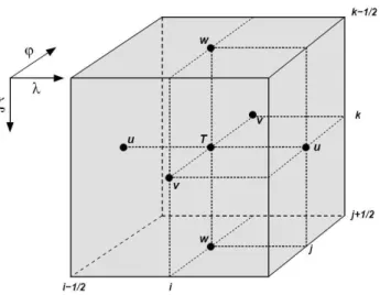
Fig. 1. Lokal Model computational grid: Arakawa C/Lorenz grid.

specific humidity, cloud liquid water, rain and snow sedi-mentation fluxes. The basic state describes a dry atmosphere at rest which is defined as horizontally homogeneous, verti-cally stratified and in hydrostatic balance. The basic tions are written in advection form and the continuity equa-tion is replaced by the prognostic equaequa-tion of the perturba-tion pressure. The Lokal Model adopts a generalized terrain-following coordinate ζ and an Arakawa C/Lorenz grid with scalars (temperature, pressure and moist variables) defined at the center of a grid box and the normal velocity components defined on the corresponding box sides (Fig. 1).

The model adopts a second order horizontal and vertical differenciating approach. Different time integration schemes are offered to the user: a leapfrog HE-VI (horizontally ex-plicit and vertically imex-plicit) time split integration scheme, a two time-level split-explicit scheme (Gassmann, 1992), a three time level 3D semi-implicit scheme (Read et al., 2000) and a two time level 3rd-order Runge-Kutta scheme with var-ious options for high-order spatial discretization (Doms and Forstner, 2004). The physics of the model is based on dif-ferent parameterization packages, e.g. a level 2.5 moist tur-bulence parameterization, a δ-two stream radiation scheme (Ritter and Geleyn, 1992) and a two layer soil model (Ja-cobson and Heise, 1982). The model includes a grid-scale cloud and precipitation scheme as well as different param-eterizations of moist convection (Tiedtke, 1989; Kain and Fritsch, 1993) . The Lokal Model offers several microphys-ical schemes spanning from the classmicrophys-ical warm rain scheme (Kessler, 1969) to a graupel scheme.

3 Numerical experiments

The study of the basic processes of intense convective pre-cipitation is addressed by performing high resolution simu-lations of deep moist convective structures over a flat surface at the interface between the meso-γ and the micro-α scales. In this way the convection dynamics can be modelled

explic-A. Parodi: Dynamics of intense convective rain cells 3

Fig. 2. Skew T diagram showing the temperature and moisture pro-files used in the simulations. In this work a surface mixing ratio qv0 = 14g/kg is assumed. Tilted solid lines represent isotherms, long dashed lines are moist adiabats while short dashed lines are dry adiabats (picture from Weisman and Klemp (1982)).

3.1 Numerical experiment 1

In this experiment the warm bubble center is placed at the point (52,80) km near the lower left corner of the domain. The wind shear profile has been chosen to highlight as much as possible the role of vertical wind shear on deep storm dy-namics (figure 3): the shear vector rotates 1800over the low-est 5 km of the atmosphere, while the wind becomes constant and one-directional above 5 km.

Firstly, by assuming a reference value of horizontal grid spacing ∆x = ∆y = 1 km and an integration time step

∆t = 1 s, the effect of different values of 4th order

numer-ical horizontal diffusion coefficient of storm dynamics has been studied. The horizontal numerical diffusion operator re-duces the effect of spurious oscillations on numerical results. As it should be most effective on waves with a wavelength of two grid intervals, solutions adopting different values of such artificial viscosity should be qualitatively similar when the specified diffusion coefficient is sufficiently small. In par-ticular, since for a generic field ψ the horizontal diffusion operator is given by:

M_ψCM = K₄h∇2(∇2ψ) (5)

a maximum value of the horizontal diffusion coefficient is

Fig. 3. Wind hodograph used in the numerical experiment 1. Winds become constant and one-directional above 5 km.

defined through linear stability considerations K_4,maxh = (∆x)

4

128∆t (6)

and the model results are compared according to three differ-ent values of K₄h = cKh

4,max, where c is the scaling

coeffi-cient (table 1).

Table 1. Three different values of scaling coefficient c for horizon-tal diffusion coefficient.

Run c

1 0.1

2 0.5

3 1.0

From a qualitative point of view these three runs gener-ate similar scenarios: the initial cell evolves into a cyclonic, right-moving supercell. The low-level vertical wind shear and cold pool circulation, in combination with the propaga-tion of internal gravity waves, promote deep lifting along the downshear portion of the gust front, with new ordinary cells generated to the north of the supercell. From an dynamical viewpoint these new cells are weaker and less persistent than the supercell.

The effects of different values of the horizontal diffusion coefficient on some quantitative aspects of deep convection dynamics are analyzed through the temporal evolution of the maximum value of vertical velocity in each run. The behav-iors are quite different especially during the first hour of sim-ulation: run 1 has a faster evolution in respect to the more dif-fusive ones, but it seems also more unstable (figure 4). Simi-lar considerations are valid for the temporal evolution of the maximum value of the horizontal wind (figure 5). The varia-tion of numerical diffusion does not affect only such simple statistics, but also the vertical and horizontal organization of

Fig. 2. Skew T diagram showing the temperature and moisture pro-files used in the simulations. In this work a surface mixing ratio qv0=14 g/kg is assumed. Tilted solid lines represent isotherms,

long dashed lines are moist adiabats while short dashed lines are dry adiabats (picture from Weisman and Klemp, 1982).

itly and it might be possible to benefit from a more detailed representation of cloud-microphysics and transport of con-vective cells with the wind field (impact of shear).

The numerical simulations are initialized considering a horizontally homogeneous atmosphere in which an axially symmetric thermal perturbation (warm bubble) of vertical radius 1400 m and horizontal radius 10 km (Weisman and Klemp, 1982, 1984) is placed. The amplitude of the temper-ature perturbation is maximum in the cell center (2◦_{C) and} gradually decreases approaching the bubble boundaries. This warm bubble acts as a triggering mechanism for deep con-vection dynamics (initial value type problem). The computa-tional domain size is 300×300×18 km with horizontal grid spacing spanning from 2 km to 1 km: finer resolution simu-lations (500 and 250 m) will be carried out at a later stage. The vertical grid spacing stretches gradually from 80 m near the bottom boundary to 500 m near the top one.

The vertical profiles of potential temperature and mois-ture inside the computational domain are defined according to Weisman and Klemp (1982, 1984). The environmental potential temperature profile is given by:

θ (z) = θ0+(θt r−θ0)( z zt r )54_, _{z ≤ z}_{t r} ₍₁₎ θ (z) = θt rexp[ g cpTt r (z − zt r)], z > zt r (2)

(4)

A. Parodi: Dynamics of intense convective rain cells 3

The environmental relative humidity profile is given by:

H (z) =1 − 3 4( z zt r )54_, _{z ≤ z}_{t r} ₍₃₎ H (z) =0.25, z > zt r (4) where zt r=12 000 m, θt r=343 K, Tt r=213 K and

θ0=300 K. A surface value of water vapour mixing

ra-tio qv0=14 g/kg is chosen. The potential temperature and

moisture profiles are shown in Fig. 2.

The experiments are run adopting Davies relaxation boundary conditions, leapfrog HE-VI time integration scheme, a 4th order linear horizontal diffusion coefficient and Rayleigh damping layers in the upper layers (z≥12 km).

The radiation parameterization is not taken into account since the radiative processes are effective on time scales much higher than those typical of the short-lived, intense deep convective cells considered in this work. The verti-cal diffusion processes are modelled through a 2.5 scheme with prognostic treatment of turbulent kinetic energy which allows the effects of subgrid-scale condensation, evaporation and thermal circulations on cell dynamics to be taken into ac-count. Finally a warm rain microphysical scheme (Kessler, 1969) is adopted.

Two numerical experiments will be discussed in the fol-lowing two sections. The first experiment will address the study of vertical wind shear effect on deep convection dy-namics. The second one, instead, will consider the case of a single convective cell developing in the absence of wind. The sensitivity of spatio-temporal properties of intense deep convective cells to computational parameters such as hori-zontal grid spacing and numerical diffusion will be investi-gated. Furthermore some preliminary comparisons between simulated and radar observed cells will be described.

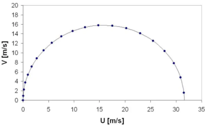
In this experiment the warm bubble center is placed at the point (52,80) km near the lower left corner of the domain. The wind shear profile has been chosen to highlight as much as possible the role of vertical wind shear on deep storm dy-namics (Fig. 3): the shear vector rotates 180◦over the lowest 5 km of the atmosphere, while the wind becomes constant and one-directional above 5 km.

Firstly, by assuming a reference value of horizontal grid spacing 1x=1y=1 km and an integration time step 1t=1 s, the effect of different values of 4th order numerical horizon-tal diffusion coefficient of storm dynamics has been stud-ied. The horizontal numerical diffusion operator reduces the effect of spurious oscillations on numerical results. As it should be most effective on waves with a wavelength of two grid intervals, solutions adopting different values of such artificial viscosity should be qualitatively similar when the specified diffusion coefficient is sufficiently small. In par-ticular, since for a generic field ψ the horizontal diffusion operator is given by:

M_ψCM =K₄h∇2(∇2ψ ) (5)

Fig. 2. Skew T diagram showing the temperature and moisture

pro-files used in the simulations. In this work a surface mixing ratio

qv0= 14g/kg is assumed. Tilted solid lines represent isotherms, long dashed lines are moist adiabats while short dashed lines are dry adiabats (picture from Weisman and Klemp (1982)).

In this experiment the warm bubble center is placed at the point (52,80) km near the lower left corner of the domain. The wind shear profile has been chosen to highlight as much as possible the role of vertical wind shear on deep storm dy-namics (figure 3): the shear vector rotates 1800over the low-est 5 km of the atmosphere, while the wind becomes constant and one-directional above 5 km.

Firstly, by assuming a reference value of horizontal grid spacing ∆x = ∆y = 1 km and an integration time step

∆t = 1 s, the effect of different values of 4th order

numer-ical horizontal diffusion coefficient of storm dynamics has been studied. The horizontal numerical diffusion operator re-duces the effect of spurious oscillations on numerical results. As it should be most effective on waves with a wavelength of two grid intervals, solutions adopting different values of such artificial viscosity should be qualitatively similar when the specified diffusion coefficient is sufficiently small. In par-ticular, since for a generic field ψ the horizontal diffusion operator is given by:

MψCM = K4h∇2(∇2ψ) (5)

a maximum value of the horizontal diffusion coefficient is

Fig. 3. Wind hodograph used in the numerical experiment 1. Winds

become constant and one-directional above 5 km.

defined through linear stability considerations

Kh 4,max=

(∆x)4

128∆t (6)

and the model results are compared according to three differ-ent values of K4h = cK4,maxh , where c is the scaling coeffi-cient (table 1).

Table 1. Three different values of scaling coefficient c for

horizon-tal diffusion coefficient.

Run c

1 0.1

2 0.5

3 1.0

The effects of different values of the horizontal diffusion coefficient on some quantitative aspects of deep convection dynamics are analyzed through the temporal evolution of the maximum value of vertical velocity in each run. The behav-iors are quite different especially during the first hour of sim-ulation: run 1 has a faster evolution in respect to the more dif-fusive ones, but it seems also more unstable (figure 4). Simi-lar considerations are valid for the temporal evolution of the maximum value of the horizontal wind (figure 5). The varia-tion of numerical diffusion does not affect only such simple statistics, but also the vertical and horizontal organization of

Fig. 3. Wind hodograph used in the numerical experiment 1. Winds become constant and one-directional above 5 km.

Table 1. Three different values of scaling coefficient c for horizon-tal diffusion coefficient.

Run c 1 0.1 2 0.5 3 1.0

a maximum value of the horizontal diffusion coefficient is defined through linear stability considerations

K_4,maxh = (1x)

4

1281t (6)

and the model results are compared according to three differ-ent values of K₄h=cK_4,maxh , where c is the scaling coefficient (Table 1).

The effects of different values of the horizontal diffusion coefficient on some quantitative aspects of deep convection dynamics are analyzed through the temporal evolution of the maximum value of vertical velocity in each run. The be-haviors are quite different especially during the first hour of simulation: run 1 has a faster evolution in respect to the more diffusive ones, but it seems also more unstable (Fig. 4). Sim-ilar considerations are valid for the temporal evolution of the maximum value of the horizontal wind (Fig. 5). The varia-tion of numerical diffusion does not affect only such simple statistics, but also the vertical and horizontal organization of the flow field. In Fig. 6, for run 1 and 2, two horizontal cross sections of the vertical velocity field, at elevation z=1000 m

(5)

Fig. 4. Temporal evolution of maximum vertical wind for different

horizontal diffusion coefficients.

Fig. 5. Temporal evolution of maximum horizontal wind for

differ-ent horizontal diffusion coefficidiffer-ents.

the flow field. In figure 6, for run 1 and 2, two horizon-tal cross sections of the vertical velocity field, at elevation z = 1000 m and timestep t = 180 minutes are compared. The flow fields look quite different especially in the upper part of the domain, where the secondary cells are different in number and localization. The reasons for such behavior are not clear at the moment and further analysis will be necessary to single out clearly the dominant mechanism responsible for the development of these secondary cells.

The effect of varying horizontal grid spacing on model re-sults has also been evaluated. In particular, a run, with hori-zontal resolution ∆x = ∆y = 2 km and an integration time step ∆t = 2 s, characterized by the same value of K4h as-sumed for run 2 has been performed. The variation in grid spacing seems to alter seriously the flow field pattern (figure 7): the coarser simulation does not show at all the develop-ment of secondary cells to the north of the supercell. Also the vertical structure of the supercell is strongly modified: the coarser simulation produces a shorter and larger super-cell (figure 8).

Fig. 6. Horizontal cross sections (z=1000 m and t=180 min of the

vertical velocities field for run 1 (upper panel) and run 2 (lower panel).

The results of experiment 1 suggest further simplification of the study case is needed. Therefore, the second experiment is about the modelling of the simplest deep convective sce-nario: the case of a single cell which develops in the absence of wind shear. A warm bubble is put in the center of the do-main so as to trigger the development of a single convective cell. By assuming the same value of K4hvalid for run 2 (ex-periment 1), the effect of horizontal grid spacing (1 km and 2 km) variation on cell evolution has been studied . Qual-itatively these two runs produce similar results: the initial cell grows and decays over the first hour with new weak cells generated as the surface cold pool first begins to spread out. These new cells, responsible for the kinks in the two

pro-Fig. 4. Temporal evolution of maximum vertical wind for different horizontal diffusion coefficients.

the flow field. In figure 6, for run 1 and 2, two horizon-tal cross sections of the vertical velocity field, at elevation

z = 1000 m and timestep t = 180 minutes are compared.

The flow fields look quite different especially in the upper part of the domain, where the secondary cells are different in number and localization. The reasons for such behavior are not clear at the moment and further analysis will be necessary to single out clearly the dominant mechanism responsible for the development of these secondary cells.

The effect of varying horizontal grid spacing on model re-sults has also been evaluated. In particular, a run, with hori-zontal resolution ∆x = ∆y = 2 km and an integration time step ∆t = 2 s, characterized by the same value of K4h

as-sumed for run 2 has been performed. The variation in grid spacing seems to alter seriously the flow field pattern (figure 7): the coarser simulation does not show at all the develop-ment of secondary cells to the north of the supercell. Also the vertical structure of the supercell is strongly modified: the coarser simulation produces a shorter and larger super-cell (figure 8).

The results of experiment 1 suggest further simplification of the study case is needed. Therefore, the second experiment is about the modelling of the simplest deep convective sce-nario: the case of a single cell which develops in the absence of wind shear. A warm bubble is put in the center of the do-main so as to trigger the development of a single convective cell. By assuming the same value of K4hvalid for run 2

(ex-periment 1), the effect of horizontal grid spacing (1 km and 2 km) variation on cell evolution has been studied . Qual-itatively these two runs produce similar results: the initial cell grows and decays over the first hour with new weak cells generated as the surface cold pool first begins to spread out. These new cells, responsible for the kinks in the two pro-Fig. 5. Temporal evolution of maximum horizontal wind for

and timestep t =180 minutes are compared. The flow fields look quite different especially in the upper part of the do-main, where the secondary cells are different in number and localization. The reasons for such behavior are not clear at the moment and further analysis will be necessary to single out clearly the dominant mechanism responsible for the de-velopment of these secondary cells.

The effect of varying horizontal grid spacing on model results has also been evaluated. In particular, a run, with horizontal resolution 1x=1y=2 km and an integration time step 1t =2 s, characterized by the same value of K₄hassumed for run 2 has been performed. The variation in grid spacing seems to alter seriously the flow field pattern (Fig. 7): the coarser simulation does not show at all the development of secondary cells to the north of the supercell. Also the verti-cal structure of the supercell is strongly modified: the coarser simulation produces a shorter and larger supercell (Fig. 8).

The results of experiment 1 suggest further simplification of the study case is needed. Therefore, the second experiment is about the modelling of the simplest deep convective sce-nario: the case of a single cell which develops in the absence

the flow field. In figure 6, for run 1 and 2, two horizon-tal cross sections of the vertical velocity field, at elevation

z = 1000 m and timestep t = 180 minutes are compared.

The flow fields look quite different especially in the upper part of the domain, where the secondary cells are different in number and localization. The reasons for such behavior are not clear at the moment and further analysis will be necessary to single out clearly the dominant mechanism responsible for the development of these secondary cells.

The effect of varying horizontal grid spacing on model re-sults has also been evaluated. In particular, a run, with hori-zontal resolution ∆x = ∆y = 2 km and an integration time step ∆t = 2 s, characterized by the same value of K4h

as-sumed for run 2 has been performed. The variation in grid spacing seems to alter seriously the flow field pattern (figure 7): the coarser simulation does not show at all the develop-ment of secondary cells to the north of the supercell. Also the vertical structure of the supercell is strongly modified: the coarser simulation produces a shorter and larger super-cell (figure 8).

The results of experiment 1 suggest further simplification of the study case is needed. Therefore, the second experiment is about the modelling of the simplest deep convective sce-nario: the case of a single cell which develops in the absence of wind shear. A warm bubble is put in the center of the do-main so as to trigger the development of a single convective cell. By assuming the same value of K₄hvalid for run 2 (ex-periment 1), the effect of horizontal grid spacing (1 km and 2 km) variation on cell evolution has been studied . Qual-itatively these two runs produce similar results: the initial cell grows and decays over the first hour with new weak cells generated as the surface cold pool first begins to spread out. These new cells, responsible for the kinks in the two pro-Fig. 6. Horizontal cross sections (z=1000 m and t=180 min of the vertical velocities field for run 1 (upper panel) and run 2 (lower panel).

of wind shear. A warm bubble is put in the center of the do-main so as to trigger the development of a single convective cell. By assuming the same value of K₄hvalid for run 2 (ex-periment 1), the effect of horizontal grid spacing (1 km and 2 km) variation on cell evolution has been studied . Qualita-tively these two runs produce similar results: the initial cell grows and decays over the first hour with new weak cells generated as the surface cold pool first begins to spread out. These new cells, responsible for the kinks in the two pro-files in Fig. 9, dissipate quickly as the cold pool continues to propagate away, with the cold pool circulation unable to produce sufficient lifting for sustaining effective cell regen-eration. However, the temporal evolution of the maximum value of vertical velocity is quite different (Fig. 9).

When the simulation is coarser, the cell is less intense, but surprisingly it presents a slower decay.

As mentioned before, part of the work is devoted to the direct comparison between spatio-temporal properties of

(6)

A. Parodi: Dynamics of intense convective rain cellsA. Parodi: Dynamics of intense convective rain cells 5 5

Fig. 7. Horizontal cross sections (z=1000 m and t=180 min) of the

vertical velocities field for 2 km run (upper panel) and 1 km run (lower panel).

files in figure 9, dissipate quickly as the cold pool continues to propagate away, with the cold pool circulation unable to produce sufficient lifting for sustaining effective cell regen-eration. However, the temporal evolution of the maximum value of vertical velocity is quite different (figure 9).

As mentioned before, part of the work is devoted to the di-rect comparison between spatio-temporal properties of simu-lated cells and radar measured cells. In fact von Hardenberg et al. (2003) have recently shown that convective rain cells over the ocean are exponential in shape. They define shape as the spatial distribution of rainfall intensity around the cell center. These findings are also confirmed by the preliminary analysis of the shape of the single rain cell considered in this

Fig. 8. Vertical cross sections (y=100 km and t=42 min) of the

experiment (figure 10).

It must be stressed that these results are really at an initial stage. A physical understanding of this behavior which

as-Fig. 9. Temporal evolution of maximum vertical velocity for

differ-ent horizontal grid spacing (1 km pink, 2 km blue).

Fig. 7. Horizontal cross sections (z=1000 m and t=180 min) of the vertical velocities field for 2 km run (upper panel) and 1 km run (lower panel).

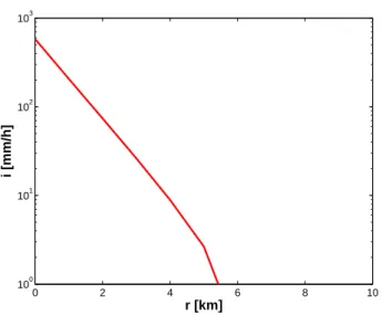
simulated cells and radar measured cells. In fact von Hard-enberg et al. (2003) have recently shown that convective rain cells over the ocean are exponential in shape. They define shape as the spatial distribution of rainfall intensity around the cell center. These findings are also confirmed by the pre-liminary analysis of the shape of the single rain cell consid-ered in this experiment (Fig. 10).

It must be stressed that these results are really at an initial stage. A physical understanding of this behavior which as-sesses, for example, its sensitivity to microphysical scheme details, needs further investigation. Besides, the dependence of the shape of rain cells on the three-dimensional spatial structure of microphysical fields will have to be analyzed.

4 Conclusions

The dynamics of deep convective cells in simplified model configurations has been investigated by using the Lokal

Fig. 7. Horizontal cross sections (z=1000 m and t=180 min) of the vertical velocities field for 2 km run (upper panel) and 1 km run (lower panel).

Fig. 8. Vertical cross sections (y=100 km and t=42 min) of the vertical velocities field for 2 km run (upper panel) and 1 km run (lower panel).

as-Fig. 9. Temporal evolution of maximum vertical velocity for differ-ent horizontal grid spacing (1 km pink, 2 km blue).

Fig. 8. Vertical cross sections (y=100 km and t=42 min) of the ver-tical velocities field for 2 km run (upper panel) and 1 km run (lower panel).

Fig. 7. Horizontal cross sections (z=1000 m and t=180 min) of the

Fig. 8. Vertical cross sections (y=100 km and t=42 min) of the

as-Fig. 9. Temporal evolution of maximum vertical velocity for

differ-ent horizontal grid spacing (1 km pink, 2 km blue).

Fig. 9. Temporal evolution of maximum vertical velocity for differ-ent horizontal grid spacing (1 km pink, 2 km blue).

Model as a numerical framework in order to obtain a deeper understanding of basic processes of intense convective pre-cipitation. The preliminary results, presented here, are promising and call for further analysis. In particular, the spatio-temporal properties of convective cells are found to be quite dependent on numerical and physical parameters such

(7)

0 2 4 6 8 10 100 101 102 103 r [km] i [mm/h]

Fig. 10. Log-linear plot of the instantaneous profile (t=39 min) of the rainfall intensity for single cell simulation: r represents the dis-tance from the cell center.

sesses, for example, its sensitivity to microphysical scheme details, needs further investigation. Besides, the dependence of the shape of rain cells on the three-dimensional spatial structure of microphysical fields will have to be analyzed.

4 Conclusions

The dynamics of deep convective cells in simplified model configurations has been investigated by using the Lokal Model as a numerical framework in order to obtain a deeper understanding of basic processes of intense convective pre-cipitation. The preliminary results, presented here, are promising and call for further analysis. In particular, the spatio-temporal properties of convective cells are found to be quite dependent on numerical and physical parameters such as numerical diffusion and horizontal grid spacing (Adler-man and Drogemeier, 2002). The work is in progress. A physical explanation of such behaviors will be carried out, also through a comparison between the characteristics of simulated convective cells and cells measured by radars. The role of other parameters (microphysical scheme, surface drag coefficient) on model performances, even at lower horizontal resolution (500-250 m), will also be evaluated. In particular The effects of these results in the understanding of deep con-vection dynamics as well as in the context of LAM numerical weather prediction will be considered.

Acknowledgements. The author is grateful to Gunther Doms for his

invaluable contribution, without which this work would not have been possible. Gratitude is also extended to A. Provenzale, J. v. Hardenberg, F. Siccardi, L. Ferraris and T. Paccagnella for their en-lighting discussions and useful comments.

References

Adlerman, E. and Drogemeier, K.: The sensitivity of numerically simulated cyclic mesocyclogenesis to variations in model physi-cal and computational parameters, Mon. Wea. Rev., 130, 2671– 2691, 2002.

Austin, P. M. and Houze, R. A.: Analysis of the structure of precipi-tation patterns in New England, J. Appl. Meteorol., 11, 926–935, 1972.

Austin, P. V. J. and Locatelli, J. D.: Rainbands, precipitation cores and generating cells in a cyclonic storm, J. Atmos. Sci., 35, 230– 241, 1978.

Bryan, G. H., Wyngaard, J. C., and Fritsch, J. M.: Resolution re-quirements for the simulation of deep moist convection, Mon. Wea. Rev., 131, 2394–2416, 2003.

Cotton, W. R. and Anthes, R.: Storm and cloud dynamics, Aca-demic Press, 1989.

Doms, G. and Forstner, J.: Development of a kilometer-scale NWP-system: LMK, COSMO Newsletter, 4, 159–167, 2004.

Doms, G. and Schaettler, U.: The nonhydrostatic limited-area model LM (Lokal-Modell) of DWD. Part I: Scientific documen-tation, Deutscher Wetterdienst (DWD), 1999.

Feral, L., Fedi, F., Magistroni, C., Paraboni, A., and Pawlina, A.: Rain cells shape and orientation distribution in Southern West France, Phys. Chem. Earth B, 25, 1073–1078, 2000.

Gassmann, A.: A two timelevel Integration Scheme for the LM, COSMO Newsletter, 2, 1992.

Houze, R. A. J. and Hobbs, P. V.: Organization and structure of pre-cipitating cloud systems, Adv. Geophysics, 24, 225–315, 1982. Jacobson, I. and Heise, E.: A new economic method for the

com-putation of the surface temperature in numerical models, Beitr. Phys. Atm., 55, 128–141, 1982.

Kain, J. S. and Fritsch, J. M.: Convective parameterization for mesoscale models: The Kain-Fritsch scheme, Meteorological Monographs, 46, 165–170, 1993.

Kessler, E.: On the distribution and continuity of water substanceon atmospheric circulation, Meteorol. Monogr., 10 (32), 1969. Klemp, J. and Wilhelmson, R.: The simulation of three-dimensional

convective storm dynamics, J. Atmos. Sci., 35, 1070–1096, 1978. Read, P. L., Thomas, N. P. J., and Risch, S. H.: An Evaluation of Eu-lerian and Semi-Lagrangian Advection Schemes in Simulations of Rotating, Stratified Flows in the Laboratory. Part I: Axisym-metric Flow, Mon. Wea. Rev., 128, 283528 521, 2000.

Ritter, B. and Geleyn, J. F.: A comprehensive radiation scheme for numerical weather prediction models with potential applications in climate simulations, Mon. Wea. Rev., 120, 303–325, 1992. Steppeler, J., Hess, R., Doms, G., Schttler, U., and Bonaventura, L.:

Review of numerical methods for nonhydrostatic weather pre-diction models, Meteorology and Atmospheric Physics, Meteo-rology and Atmospheric Physics, 82, 287–301, 2003.

Szoke, E., Zipser, E., and Jorgensen, D.: A radar study of convective cells in GATE. Part I: Vertical profile statistics and comparison with hurricane cells., J. Atmos. Sci., 43, 184197, 1986.

Tiedtke, M.: A comprehensive mass flux scheme for cumulus pa-rameterization in large scale models., Mon. Wea. Rev., 117, 1779–1800, 1989.

von Hardenberg, J., Provenzale, A., and Ferraris, L.: The shape of rain cells, Geophys. Res. Lett., 30, 10.1029/2003GL018 539, 2003.

Weisman, M. L. and Klemp, J.: The dependence of of numerically simulated convective storms on vertical wind shear and buoy-ancy, Mon. Wea. Rev., 110, 504–520, 1982.

Fig. 10. Log-linear plot of the instantaneous profile (t=39 min) of the rainfall intensity for single cell simulation: r represents the dis-tance from the cell center.

as numerical diffusion and horizontal grid spacing (Adler-man and Drogemeier, 2002). The work is in progress. A physical explanation of such behaviors will be carried out, also through a comparison between the characteristics of simulated convective cells and cells measured by radars. The role of other parameters (microphysical scheme, surface drag coefficient) on model performances, even at lower horizontal resolution (500–250 m), will also be evaluated. In particular The effects of these results in the understanding of deep con-vection dynamics as well as in the context of LAM numerical weather prediction will be considered.

Acknowledgements. The author is grateful to G. Doms for his

invaluable contribution, without which this work would not have been possible. Gratitude is also extended to A. Provenzale, J. v. Hardenberg, F. Siccardi, L. Ferraris and T. Paccagnella for their enlighting discussions and useful comments.

Edited by: L. Ferraris

Reviewed by: anonymous referees