Dynamic treatment regimens for congestive heart failure

Dynamic Treatment Regimens for Congestive Heart

Failure

by

Katherine W. Young

B.S., Massachusetts Institute of Technology (2018)

Submitted to the Department of Electrical Engineering and Computer

Science

in partial fulfillment of the requirements for the degree of

Master of Engineering in Electrical Engineering and Computer Science

at the

MASSACHUSETTS INSTITUTE OF TECHNOLOGY

February 2020

c

○ Massachusetts Institute of Technology 2020. All rights reserved.

Author . . . .

Department of Electrical Engineering and Computer Science

January 29, 2020

Certified by . . . .

Collin M. Stultz

Professor of Electrical Engineering and Computer Science

Thesis Supervisor

Accepted by . . . .

Katrina LaCurts

Chair, Master of Engineering Thesis Committee

Dynamic Treatment Regimens for Congestive Heart Failure

by

Katherine W. Young

Submitted to the Department of Electrical Engineering and Computer Science on January 29, 2020, in partial fulfillment of the

requirements for the degree of

Master of Engineering in Electrical Engineering and Computer Science

Abstract

Each year, millions of patients are hospitalized with a diagnosis of congestive heart failure (CHF). This condition is characterized by inadequate tissue perfusion resulting from an inability of the heart to provide enough blood to meet the body’s metabolic demands. Patients with CHF remain at a greater risk for mortality and other ad-verse events. A primary symptom of CHF is fluid overload ("congestion"), which is routinely treated with diuretic therapy. However, choosing a diuretic therapy that maximizes the therapeutic effects while minimizing harmful side effects remains a challenge. In order to assess a patient’s response to a particular therapy and guide future treatment decisions, clinicians monitor a number of variables including a pa-tients’ vital signs, glomerular filtration rate (GFR, a measure of renal function), and fluctuations in volume status. Nevertheless, these variables are typically insufficient by themselves to ensure that a given therapy is optimal for a given patient. Current guidelines for heart failure management were developed, in part, from large clinical trials. However, it is not always clear how to apply these observations to a given pa-tient, whose clinical characteristics may differ significantly from those of the patients in the original studies. Therefore, there is a need for methods that identify patient-specific treatments that would allow physicians to construct therapies that are truly personalized. This work describes an approach for building dynamic treatment reg-imens (DTRs) - a set of patient-specific treatment rules that optimize an outcome of interest. The method uses artificial neural networks to suggest diuretic doses that will improve a patient’s volume status while simultaneously minimizing harmful side effects on renal function. This body of work suggests the potential that DTRs have in developing personalized diuretic regimens to improve the clinical outcomes of CHF patients.

Thesis Supervisor: Collin M. Stultz

Acknowledgments

I cannot thank my advisor, Collin Stultz, enough for all of his support, guidance, and invaluable mentorship over the past 19 months. Because of him, the way I approach research and communicate it to others will never be the same. I will always be thankful for his unwavering support of my education as well as my career goals. He has shown me how it is possible not just to pursue, but to excel in, medicine and computer science simultaneously. Working with him has been the prime source of my passion to pursue a career in both fields.

I would like to express my gratitude to Manohar Ghanta and Sean Bullock of the MGH CDAC team for helping me with data procurement, and to John Guttag and Charlie Sodini for leading interdisciplinary group meetings. I would also like to thank Dr. Brandon Westover and Dr. Aaron Aguirre for helping me see the big picture and clinical motivation behind this work.

I want to extend a word of thanks to the members of the Computational Car-diovascular Research Group: Daphne Schlesinger, for being a great officemate and co-organizer of the Computational Medicine and Healthcare Reading Group; Erik Reinertsen, for all of the career advice, papers, and podcasts; Paul Myers, for helping me get started in the lab; and Aniruddh Raghu and Wangzhi Dai, for the advice in statistics and machine learning. I am also very thankful for Megumi Masuda-Loos, who has been an invaluable resource to the group.

Lastly, I want to thank my family and friends for always being there for me and supporting me through undergrad and M. Eng. My time at MIT was made incredibly special because of each one of you.

Contents

1 Congestive Heart Failure 13

1.1 Pathophysiology of Congestive Heart Failure . . . 14

1.2 Treatment of Congestive Heart Failure . . . 16

1.3 Motivation and Problem Statement . . . 18

2 Reinforcement Learning 21 2.1 Dynamic Treatment Regimens and Q-Learning . . . 21

2.2 Iterative Q-Learning . . . 23

2.3 Estimating Dynamic Treatment Regimens from Observational Datasets 25 3 Results 29 3.1 Dataset . . . 29

3.1.1 Covariates . . . 29

3.1.2 Daily Clinical Features . . . 30

3.1.3 Diuretic and Non-Diuretic Medications . . . 31

3.1.4 Clinical Outcomes . . . 31

3.2 Generating Q-Functions to Predict Clinical Outcomes . . . 34

3.3 Diuretic Optimization and Evaluation . . . 35

4 Summary and Conclusions 41 4.1 Conclusions . . . 41

5 Methods 45

5.1 Dataset Curation and Preprocessing . . . 45

5.1.1 Admitting Diagnosis and Comorbid Diseases . . . 45

5.1.2 Feature Selection . . . 46

5.1.3 Preprocessing Pipeline . . . 46

5.2 Machine Learning Methods . . . 47

5.2.1 Artificial Neural Networks . . . 47

5.2.2 Recurrent Neural Networks . . . 48 A Previous Prediction Tasks and Q-Functions 53 B Additional Method for Diuretic Optimization 55

List of Figures

1-1 Frank-Starling law relating stroke volume (SV) and left ventricular

end-diastolic pressure (LVEDP) [1] . . . 15

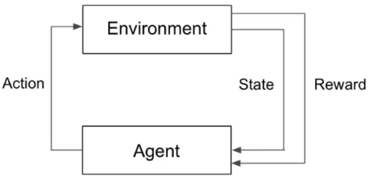
2-1 General reinforcement learning framework . . . 22

3-1 Dry weights, admission weights, and discharge weights for all encoun-ters in dataset 1, with averages denoted in the insets . . . 32

3-2 Admission creatinine and discharge creatinine levels for all encounters in dataset 1, with averages denoted in the insets . . . 34

3-3 Optimization results for weight (A), creatinine (B), and combined (C) outcomes . . . 37

3-4 Evaluation of optimization results for creatinine, weight, and combined outcomes; distance refers to the Euclidean distance between the opti-mal and actual diuretic regimens . . . 39

5-1 Pipeline for dataset 1 (A) and dataset 2 (B) . . . 48

5-2 Feedforward neural network . . . 49

5-3 Recurrent neural network schematic . . . 49

5-4 Neural network model architecture . . . 51

B-1 Optimization results (without zeroing out diuretics) for creatinine, weight, and combined outcomes . . . 56

B-2 Evaluation of optimization results (without zeroing out diuretics) for creatinine, weight, and combined outcomes; distance refers to the Eu-clidean distance between the optimal and actual diuretic regimens . . 57

List of Tables

1.1 CHF medication classes, examples, and primary physiologic effects . . 18

3.1 Binary covariate distributions in datasets 1 and 2; number and per-centages are shown for encounters and patients with positive covariate values (i.e. female, age ≥ 65, with CKD diagnosis, with COPD diag-nosis, with smoking diagnosis) . . . 30

3.2 Continuous covariate distributions in datasets 1 and 2 for encounters 31 3.3 Diuretic CHF medications included in the feature set . . . 32

3.4 Non-diuretic CHF medications included in the feature set . . . 33

3.5 Outcome distribution in dataset 1 . . . 33

3.6 Results for prediction of clinical outcomes . . . 35

3.7 Most common diuretic treatments for day 3 in dataset 1 . . . 36

5.1 Neural network variable descriptions and dimensions . . . 51

5.2 Grid search for neural network with 2 hidden layers in the RNN . . . 51

Chapter 1

Congestive Heart Failure

Heart failure (HF) affects nearly 6.2 million Americans, with annual direct costs estimated at $30 billion in 2018. It is the leading cause for hospitalizations among patients over the age of 65, and inpatient mortality rates can be as high as 25% in high-risk subpopulations [2]. Moreover, inpatient admissions account for over one-half of the financial burden. With the rising prevalance of heart disease in the United States, it is projected that over 8 million Americans will have HF by the year 2030 [3], [4].

Common symptoms of patients with congestive heart failure (CHF) include dys-pnea (shortness of breath) and lower extremity swelling secondary to fluid retention. The treatment of patients with CHF requires a dynamic assessment of volume status, renal function, electrolyte balance, as well as concomitant co-morbidities. A mainstay for the treatment of the symptoms associated with CHF is diuretic therapy, However, balancing the therapeutic benefits of diuretics with their adverse effects on the kidneys is a notoriously difficult problem. For example, while high doses of a diuretic would expedite fluid removal and consequently relieve symptoms quickly, this approach has the potential to significantly worsen renal function, especially in patients who have baseline renal dysfunction. On the other hand, prescribing a diuretic that is not po-tent enough may result in inadequate diuresis, and ultimately a longer stay in the hospital. For a health care professional, learning how to strike the perfect balance is key to providing care that maximizes good outcomes while simultaneously minimizing

future adverse events. Reinforcement learning provides a platform for learning such personalized treatment decisions using large datasets that catalog a plethora of past clinical decisions and outcomes.

This thesis is organized as follows: Chapter 1 focuses on the pathophysiology and treatment of CHF, and concludes with the problem statement. Chapter 2 presents an overview of reinforcement learning (RL), Q-learning, and dynamic treatment regimens (DTRs). Chapter 3 describes the results of this work: namely, the novel dataset, the performance of the prediction tasks, and an evaluation of the treatment decisions recommended by the algorithm. Chapter 4 offers a summary of the findings and potential future directions. Finally, Chapter 5 describes the methods used in this work.

1.1

Pathophysiology of Congestive Heart Failure

CHF is defined as the inability of the heart to provide sufficient blood flow to meet the metabolic demands of the body ("forward failure"), the inability of the heart to pump all of the blood that enters the heart ("backwards failure"), or both. CHF is characterized not only by insufficient tissue perfusion, but also by the changes resulting from the body’s attempts to compensate for the inadequate perfusion. In order to understand the pathophysiology of CHF, one must first consider the variables of cardiac output (CO), stroke volume (SV), and heart rate (HR).

CO is the volume of blood pumped by the heart per minute, and is determined by the SV and HR (Equation 1.1).

𝐶𝑂 = 𝑆𝑉 × 𝐻𝑅 (1.1)

SV is determined by the preload, contractility, and afterload. The preload, or the left ventricular end-diastolic pressure (LVEDP), refers to the filling pressure of the heart at the end of diastole. The Frank-Starling law characterizes the relationship between SV and LVEDP, and states that as the LVEDP increases, SV increases up to an asymptote (Figure 1-1) [1]. Afterload is a measure of the resistance that the heart

Figure 1-1: Frank-Starling law relating stroke volume (SV) and left ventricular end-diastolic pressure (LVEDP) [1]

must overcome to pump blood; it is proportional to the systemic vascular resistance (SVR), mean aortic pressure, and pulmonary arterial pressure. Contractility refers to the strength with which the ventricle contracts to eject blood. The Frank-Starling law also states that for a given LVEDP, the SV increases with cardiac contractility (Figure 1-1) [1].

Given these definitions, we now discuss the underlying mechanisms for the patho-physiology of CHF.

CHF can arise from systolic dysfunction, diastolic dysfunction, or both. With systolic dysfunction, the pathophysiology can arise from reduced cardiac contractility and stroke volume (i.e. myocardial infarction), increased afterload (i.e. hypertension, aortic stenosis), increased preload (i.e. backflow into the LV), arrhythmias, and valvu-lar diseases. With an increased afterload, the heart must pump against a greater load. A subtype of HF, known as high-output HF, is characterized by elevated CO. This condition results as a consequence of inadequate tissue perfusion from HF, whereby the CO is elevated to attempt to restore tissue perfusion.

With diastolic dysfunction, loss of elasticity (decrease compliance) or impaired re-laxation of the ventricles (i.e. by LV hypertrophy) reduces ventricular filling, thereby reducing SV and CO.

failure of the heart. In forward failure, the heart is unable to provide sufficient for-ward blood flow to the rest of the body. This results in organ dysfunction (including renal dysfunction) and hypotension. In backwards failure, an elevated preload (i.e. left ventricular end-diastolic pressure, LVEDP), causes blood to seep into the lungs. The resulting increase in pulmonary capillary pressure causes fluid to seep into the interstitium and alveoli, resulting in pulmonary edema. This fluid buildup interferes with oxygen exchange in the alveoli to cause shortness of breath. Furthermore, be-cause the heart is unable to pump all of the blood it receives, blood builds up in the periphery to cause systemic venous congestion. As a result, fluid seeps out of the blood vessels and pools in the periphery (i.e. feet, ankles, legs), causing edema and weight gain.

In a CHF patient, the body attempts to compensate for inadequate tissue per-fusion through a number of mechanisms. Reduced tissue perfusion activates the compensatory mechanisms of the neurohormonal system through the baroreceptor re-sponse to falling blood pressure (BP). The sympathetic nervous system is stimulated, thereby increasing HR, BP, and contractility. The renin-angiotensin-aldosterone sys-tem (RAAS) is also activated in response to a decrease in renal perfusion following decreased CO. Other compensatory mechanisms include physical remodeling of the heart (i.e. LV dilation, LV hypertrophy). In the short term, these compensatory mechanisms help to improve CO, but over time, prolonged activation can result in myocyte death, as well as dysfunction of the heart, lungs, kidneys, and other organs [5].

1.2

Treatment of Congestive Heart Failure

Management of CHF depends on the stage and severity of the disease. The different classes of CHF medications, and examples of each, are summarized in Table 1.1 [6]. Many CHF therapies aim to manage the neurohormonal response to prevent long-term complications. In particular, they work to reverse the excessive rise in preload, afterload, HR, and catecholamines that arise from the compensatory neurohormonal

response.

Diuretics are a separate class of medications used to treat the fluid retention asso-ciated with CHF. The goal of diuretic therapy is to achieve and maintain euvolemia, or a patient’s dry weight. The dry weight refers to the normal body weight, or body weight without excess fluid.

Diuretics work by promoting urine output from the kidney (diuresis), primarily by inhibiting sodium reabsorption at different segments of the kidney. Diuretic ther-apy varies from patient to patient, and can include one (monotherther-apy) or multiple (combination therapy) diuretic medications. Typically, diuretics are started at low doses and titrated up as needed and as tolerated. The therapeutic effects of diuret-ics can be quantified by an increase in urine output and a corresponding decrease in weight. These markers should be monitored daily to determine the appropriate dosing strategy.

Though effective for treating the congestive symptoms of CHF, diuretic therapy also comes with a host of side effects, including renal dysfunction. The glomerular filtration rate provides a measure of renal function and is defined as the volume of fluid filtered by the kidney per unit time. The gold standard method of measuring GFR involves injecting inulin into the blood and measuring its clearance by the kidneys. However, this method is invasive and expensive. The creatinine clearance rate, or the volume of blood plasma that is cleared of creatinine per unit time, provides a cheaper and quicker estimate of the GFR. Creatinine is a waste product of creatine phosphate metabolism in muscle tissues, and serum creatinine levels can be used to estimate the creatinine clearance rate (high levels of serum creatinine are indicative of renal dysfunction). This estimate of the creatinine clearance rate provides an estimate of the GFR (eGFR) [7].

Diuretic use is associated with a decrease in GFR (renal function). Removing too much volume through urine excretion significantly reduces the EDV, and therefore the LVEDP (the two are related by the LV compliance), leading to a reduction in renal blood flow and GFR. In this way, diuretic therapies can lead to renal dysfunction.

Table 1.1: CHF medication classes, examples, and primary physiologic effects Class Examples Physiologic Effects Angiotensin-converting

enzyme (ACE) inhibitors

Lisinopril, captopril,

enalapril Vasodilation, reduced BP Angiotensin II

receptor blockers

Losartan, valsartan,

candesartan Vasodilation, reduced BP Beta blockers

Carvedilol, metoprolol,

bisoprolol Reduced HR and BP Vasodilators

Hydralazine,

isosorbide dinitrates Vasodilation I(f) inhibitor Ivabradine Reduced HR Digoxin Digoxin

Increased cardiac

contractility, reduced HR Angiotensin

receptor-neprilysin inhibitor Sacubitril/valsartan Vasodilation, reduced BP

Diuretics

Furosemide, bumetanide, torsemide, metolazone, amiloride, chlorothiazide, hydrochlorothiazide,

triamterene, spironolactone Increased urine production

About two-thirds of hospitalized CHF patients are estimated to have chronic kidney disease (CKD) as defined by an estimated GFR of <60 ml/min/1.73 m2 _{[8]. Thus,}

it is extremely important to consider the adverse effects of diuretic therapy on renal function. Daily monitoring of weight, electrolyte balance, and renal function can help to detect adverse effects and adjust the diuretic therapy as needed.

1.3

Motivation and Problem Statement

Given a patient’s medical history and clinical presentation, how should a physician construct an effective treatment regimen - one that achieves the maximum therapeutic effect while minimizing negative side effects? We seek to answer this question through the development of dynamic treatment regimens (DTRs), a set of treatment rules designed to optimize a particular outcome. In this work, we aim to optimize three clinical outcomes before discharge:

1. Outcome A: Has the patient been sufficiently diuresed to at least halfway to their dry weight?

2. Outcome B: Has the patient’s serum creatinine improved from baseline, or is it within the normal range (0.6-1.2 mg/dL in males and 0.5-1.1 mg/dL in females)? 3. Outcome C: Are both Outcomes A and B satisfied?

Our goal is to provide clinical decision support in choosing diuretic therapies for heart failure patients: we aim to create a computational model that will learn from past treatment decisions and patient outcomes to build a set of safe and effective treatment rules.

Chapter 2

Reinforcement Learning

Precision medicine, whereby medical therapies are tailored to the individual patient based on their unique characteristics, has witnessed growing interest and progress in recent years. Differences in clinical phenotypes, medical histories, and comorbid diseases lead to diverse responses to treatment therapy, highlighting the need for individualized treatment plans.

Reinforcement learning (RL) techniques have shown promise in tackling these se-quential decision-making problems in various clinical settings, including therapies for mental health disorders [9], cancer trial design [10], and sepsis management [11]. Re-inforcement learning is an area of machine learning in which a virtual agent interacts with an environment to learn a set of rules, with the goal of maximizing an expected cumulative reward (Figure 2-1) [12]. In the clinical setting, a physician strives to make decisions about what therapies to give, how much, and when, to maximize a patient’s probability of achieving a desired outcome.

2.1

Dynamic Treatment Regimens and Q-Learning

A set of treatment rules chosen to optimize a particular outcome for each individual patient is known as a dynamic treatment regimen (DTR). A treatment rule at a given time-step dictates whether to give a medication or perform an intervention at that time. The treatment plan for a given patient may change over time as their

Figure 2-1: General reinforcement learning framework

trajectory (clinical history) evolves over time - hence the descriptor "dynamic." As each treatment decision depends on a patient’s unique covariates, clinical history, and treatment history, DTRs account for heterogeneity across patients as well as across time. Given this platform for solving sequential decision-making problems, RL provides a suitable framework for estimating DTRs.

Estimating DTRs can be framed in terms of solving a Markov Decision Process (MDP). An MDP is described by a set of possible states 𝑆, a set of possible actions 𝐴, a set of transition probabilities 𝑝(𝑠′|𝑠, 𝑎) where 𝑠′_{is the resulting state after performing}

action 𝑎 in state 𝑠, a reward function 𝑅(𝑠, 𝑎) which gives the immediate reward attained from taking action 𝑎 in state 𝑠, and a discount factor 𝛾 that quantifies the relative weighting of future rewards. An MDP assumes the Markov Property: given a current state and action, the next state depends only on the current state and action and not on the prior history.

We define a policy 𝜋 : 𝑆 → 𝐴 to be a function that specifies the action 𝜋(𝑠) to take while in state 𝑠. The goal is to choose a policy 𝜋* that maximizes the expected value of the return, or the future cumulative discounted reward:

𝜋* = arg max 𝜋 E[ ∞ ∑︁ 𝑗=0 𝛾𝑗𝑅(𝑠𝑗, 𝑎𝑗)|𝜋] (2.1) ,

One widely used algorithm for finding the optimal policy is Q-learning, which remains popular for its relative simplicity and flexibility in implementation [13], [14]. Moreover, it enables learning even in cases where the transition function or probability distribution of the random variables is unknown.

Q-learning involves updating a Q-function, which maps each state-action pair to its expected reward (called a Q-value), given that the optimal policy is followed thereafter. When the agent takes action 𝑎 in state 𝑠, an update to the Q-value for that (𝑠, 𝑎) pair is made according to Equation 2.2:

𝑄(𝑠, 𝑎) ← 𝑄(𝑠, 𝑎) + 𝛼[𝑅(𝑠, 𝑎) + 𝛾 max

𝑎′∈𝐴

(𝑄(𝑠′, 𝑎′)) − 𝑄(𝑠, 𝑎)] (2.2) where 𝛼 is the learning rate and 𝛾 is the discount factor. Following sufficient exploration of the state-action space (assuming finite state and action spaces), the algorithm converges and the optimal policy can be derived according to Equation 2.3. For any state 𝑠, the optimal action can be calculated as:

𝜋*(𝑠) = arg max

𝑎∈𝐴 𝑄(𝑠, 𝑎). (2.3)

2.2

Iterative Q-Learning

In traditional Q-learning, a table of Q-values for each (𝑠, 𝑎) pair is maintained and updated during the online learning process. In settings with large (i.e. continuous or discrete) state and action spaces, a tabular approach becomes impractical. Moreover, in the medical domain, having an agent interact with the environment by exploring actions can pose a risk to patients. By using a function to approximate the Q-function from observational data, an optimal policy can be learned without direct exploration. Here, we describe a version of Q-learning called iterative Q-learning that is readily applied to observational datasets with large state and action spaces. Iterative Q-learning uses backwards induction to generate a different Q-function 𝑄𝑗 for each

time-step 𝑗, instead of one Q-function for all time-steps. Iterative Q-learning starts from the last time-step and works via backward induction to estimate the best action

at each time-step by optimizing interval-specific Q-functions, 𝑄𝑗, for 𝑗 = 1, ..., 𝑘.

The first iteration, which corresponds to the last time-step 𝑘, produces an approx-imation of the 𝑄𝑘-function. As the true 𝑄𝑘-values are the expectation of the reward

conditioned on (𝑠𝑘, 𝑎𝑘), the 𝑄𝑘-function can be approximated using Equation 2.4:

𝑄𝑘(𝑠, 𝑎) = 𝐸[𝑟𝑘|𝑠𝑘 = 𝑠, 𝑎𝑘= 𝑎] (2.4)

where (𝑠𝑘, 𝑎𝑘) pairs are the inputs and the final rewards 𝑟𝑘are the target outputs.

Subsequent Q-functions are derived in an iterative fashion using approximations from the previous Q-function. In this way, the 𝑗𝑡ℎ_{Q-function (𝑄}

𝑗) is similarly derived

using a regression algorithm, with (𝑠𝑗, 𝑎𝑗) pairs as the inputs and

𝑟𝑗 + 𝛾 𝑚𝑎𝑥

𝑎∈𝐴 𝑄𝑗+1(𝑠𝑗+1, 𝑎) as the target outputs. Essentially, 𝑄𝑗 is an expectation of

the cumulative reward conditioned on the agent taking an optimal action in all future time-steps.

Note that in our problem formulation, we do not define intermediate rewards 𝑟𝑗

for 𝑗 = 1, ..., 𝑘. The only nonzero reward is achieved at the last time-step. In this slightly modified setting, 𝛾 = 1 and 𝑟𝑗 = 0 ∀ 𝑗 ̸= 𝑘.

The optimal policy can be derived in a similar manner to Q-learning by selecting the actions that result in the highest Q-values at each time-step.

Any type of function approximator (i.e. linear regression, support vector machines, random forests) may be used to approximate each 𝑄𝑗. This work uses an artificial

neural network (ANN) as the function approximator.

There are certain differences in terminology between standard RL and RL applied to DTRs. An "action" corresponds to a treatment decision in a DTR. The "state" refers to the clinical observations (and covariates) of a patient, also referred to as a clinical history. The final "reward" is equivalent to the probability of an encounter achieving a desired outcome. Finally, the optimal "policy" corresponds to the set of optimal treatment rules learned, or the DTR.

2.3

Estimating Dynamic Treatment Regimens from

Observational Datasets

In the early 2000s, Lavori and Dawson introduced the concept of Sequential Multi-ple Assignment Randomized Trials (SMART) for the generation of DTRs [15], [16]. SMART studies represent a multi-stage randomized experimental approach, in which subjects are randomly assigned treatments at each stage. SMART has been widely implemented, especially in cancer research [10]. However, conducting multi-staged randomized trials can be costly. Moreover, the exploratory nature of RL may raise concerns about patient health and safety, especially in the case of complex, exper-imental trials. For these reasons, the initial development of DTRs (which can be subsequently validated by randomized trials) from large observational datasets pro-vide offer an alternative to implementing traditional randomized trials from the start. In these non-randomized settings, it is important that all confounding covariates are accounted for by the RL model. Various methods of incorporating confound-ing variables, from direct adjustment to propensity scorconfound-ing (i.e. inverse probability weighted estimators), have been studied [14]. In a 2012 work on estimating DTRs from observational data, Chakraborty and Moodie recommended the direct incorpo-ration of covariates into the RL models to account for the non-randomized nature of these datasets. This is the approach used in our work.

We now present the approach we employ for estimating DTRs using iterative Q-learning. For a DTR with 𝑘 time-steps, we define three random variables: the observable clinical histories ⃗𝑂, the covariates ⃗𝐶, and the actions ⃗𝐴. The history ⃗𝐻 is a vector comprising ⃗𝑂 and ⃗𝐶. The outcome, Y, is a random variable. There is a distinction between the outcome, Y, and the reward, 𝑃 (𝑌 = 1| ⃗𝐻, ⃗𝐴). The goal is to calculate optimal decision rules, (𝑑1, 𝑑2, ..., 𝑑𝑘), where 𝑑𝑗 = 𝑑𝑗( ⃗𝐻𝑗) =

ˆ ⃗ 𝐴𝑗, for

𝑗 = 1, 2, ..., 𝑘.

In this work, the 𝑗th Q-function gives an expectation of the final outcome given a patient’s clinical history up to time-step 𝑗, assuming that all future treatment decisions are optimal (Equations 2.5, 2.6, 2.7).

𝑄𝑘( ⃗𝐻𝑘, ⃗𝐴𝑘) = 𝐸[𝑌 | ⃗𝐻𝑘, ⃗𝐴𝑘] (2.5) 𝑄𝑘−1( ⃗𝐻𝑘−1, ⃗𝐴𝑘−1) = 𝐸[𝑚𝑎𝑥 ⃗ 𝑎𝑘 (𝑄𝑘( ⃗𝐻𝑘, ⃗𝑎𝑘))| ⃗𝐻𝑘−1, ⃗𝐴𝑘−1] (2.6) ... 𝑄1( ⃗𝐻1, ⃗𝐴1) = 𝐸[𝑚𝑎𝑥 ⃗𝑎2 (𝑄2( ⃗𝐻2, ⃗𝑎2))| ⃗𝐻1, ⃗𝐴1] (2.7)

Algorithm

Here, we adapt the iterative Q-learning algorithm for generating DTRs using a set of 𝑛 encounters. Let the 𝑗th Q-function, 𝑄𝑗, be parametrized by 𝜃𝑗.

1. Train a neural network to estimate the best parameters ˆ𝜃𝑘for time-step 𝑘, which

fully define 𝑄𝑘. Note that the loss function 𝐿 depends on the problem. In this

work, the binary cross-entropy loss was used (Equation 5.2). (ˆ𝜃𝑘) = arg min

^ 𝜃𝑘

𝐿 (𝑌, 𝑄𝑘( ⃗𝐻𝑘, ⃗𝐴𝑘, ˆ𝜃𝑘)) (2.8)

2. Find the pseudo-outcomes ˆ𝑌𝑘−1.

ˆ

𝑌𝑘−1 = max ⃗𝑎𝑘

𝑄𝑘( ⃗𝐻𝑘, ⃗𝑎𝑘, ˆ𝜃𝑘) (2.9)

3. Train a neural network to estimate the best parameters ˆ𝜃𝑘−1 for time-step 𝑘 − 1,

which fully define 𝑄𝑘−1.

(ˆ𝜃𝑘−1) = arg min ^ 𝜃𝑘−1

𝐿 ( ˆ𝑌𝑘−1, 𝑄𝑘−1( ⃗𝐻𝑘−1, ⃗𝐴𝑘−1, ˆ𝜃𝑘−1)) (2.10)

4. Repeat steps 2-3 until reach 𝑗 = 1.

5. The optimal treatment rule 𝑑𝑗 for time-step 𝑗 can be calculated as:

𝑑𝑗( ⃗𝐻𝑗) = arg max ⃗ 𝐴𝑗

𝑄𝑗( ⃗𝐻𝑗, ⃗𝐴𝑗, ˆ𝜃𝑗) (2.11)

Chapter 3

Results

3.1

Dataset

Dataset 1 includes 617 encounters (522 patients) with admission dates ranging from April 2016 to October 2018. Dataset 2 includes 62 encounters (53 patients) with admission dates ranging from June 2018 to October 2019. Dataset 1 was used to train and select the models for constructing the DTRs. Dataset 2 was used as a holdout set to evaluate the DTRs on patients that the models had not seen. There was no overlap between the two datasets.

3.1.1

Covariates

The 9 covariates included were gender, age, prior diagnosis of chronic kidney disease (CKD), prior diagnosis of chronic obstructive pulmonary disease (COPD), prior di-agnosis of smoking, dry weight estimate, average prior serum creatinine, weight at admission, and amino-terminal pro-B-type natriuretic peptide (NT-proBNP) at ad-mission. NT-proBNP is an example of a natriuretic peptide that is released as a response to hypertrophy, fluid overload, and ventricular wall stress. NT-proBNP is typically increased in patients with CHF and is used as a clinical marker in diagnosis and prognosis [17].

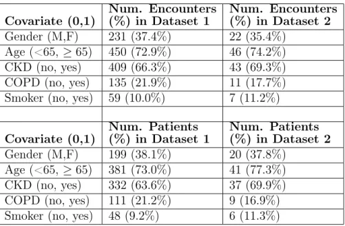
Table 3.1: Binary covariate distributions in datasets 1 and 2; number and percentages are shown for encounters and patients with positive covariate values (i.e. female, age ≥ 65, with CKD diagnosis, with COPD diagnosis, with smoking diagnosis)

Covariate (0,1) Num. Encounters (%) in Dataset 1 Num. Encounters (%) in Dataset 2 Gender (M,F) 231 (37.4%) 22 (35.4%) Age (<65, ≥ 65) 450 (72.9%) 46 (74.2%) CKD (no, yes) 409 (66.3%) 43 (69.3%) COPD (no, yes) 135 (21.9%) 11 (17.7%) Smoker (no, yes) 59 (10.0%) 7 (11.2%) Covariate (0,1) Num. Patients (%) in Dataset 1 Num. Patients (%) in Dataset 2 Gender (M,F) 199 (38.1%) 20 (37.8%) Age (<65, ≥ 65) 381 (73.0%) 41 (77.3%) CKD (no, yes) 332 (63.6%) 37 (69.9%) COPD (no, yes) 111 (21.2%) 9 (16.9%) Smoker (no, yes) 48 (9.2%) 6 (11.3%)

all prior weights in the dataset taken in an outpatient setting or upon a previous discharge. The average prior serum creatinine for a patient was calculated as the average of all previous serum creatinine values for that patient available in the dataset. The majority of encounters/patients were male and at least 65 years of age. Around two-thirds of the patients had a prior diagnosis of CKD, whereas one-fifth of the patients had a prior diagnosis of COPD. About one-tenth of the patients had a history of smoking. The distributions of the binary covariates for both datasets are provided in Table 3.1; information is shown for both encounters and patients. The distributions of the continuous covariates for both datasets are provided in Table 3.2; as these covariates are encounter-specific, the data are only shown for encounters.

3.1.2

Daily Clinical Features

Two of the most important clinical variables for monitoring CHF patients are weight and creatinine. Weight changes are reflective of the effectiveness of the diuretic regi-men, while the serum creatinine is a measure of a patient’s renal function. Additional

Table 3.2: Continuous covariate distributions in datasets 1 and 2 for encounters Covariate Mean ± Stdev in Dataset 1 Mean ± Stdev in Dataset 2 Dry weight 74.7 ± 20.9 kg 81.1 ± 29.9 kg Average prior serum creatinine 1.6 ± 0.9 mg/dL 1.7 ± 0.7 mg/dL Admission weight 85.7 ± 23.4 kg 93.2 ± 34.1 kg

Admission NT-ProBNP 8796 ± 15002 pg/mL 7985 ± 10355 pg/mL

features selected were potassium, glucose, calcium, sodium, anion gap, chloride, BUN, and CO2 (see Chapter 4 for feature selection methods).

3.1.3

Diuretic and Non-Diuretic Medications

Twenty-one diuretic CHF medications and 24 non-diuretic CHF medications were cho-sen as features for the model (see Chapter 4 for selection methods). Each medication and its administration route was considered a separate feature (e.g. bumetanide tablet was considered differently from bumetanide injection) because orally administered di-uretics must be absorbed by the gut before entering the bloodstream. Depending on the gut profile of the patient and the bioavailability of the drug, the absorption of oral diuretics may differ between diuretics and between patients.

Each dose was normalized by the maximum dose for that medication given in the first three days, across all encounters in Dataset 1.

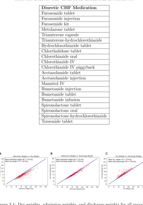
The 21 diuretic CHF medications and 24 non-diuretic CHF medications are shown in Tables 3.3 and 3.4, respectively.

3.1.4

Clinical Outcomes

The distribution of outcomes in Dataset 1 is shown in Table 3.5.

These data are also presented in Figures 3-1 and 3-2. Figure 3-1A shows that at admission, all patients in the dataset are at or above their dry weight - an expected finding given that this was one criterion used to create the cohort. Figure 3-1B shows that most patients’ discharge weights are lower than their admission weights: the

Table 3.3: Diuretic CHF medications included in the feature set Diuretic CHF Medication Furosemide tablet Furosemide injection Furosemide kit Metolazone tablet Triamterene capsule Triamterene-hydrochlorothiazide Hydrochlorothiazide tablet Chlorthalidone tablet Chlorothiazide oral Chlorothiazide IV Chlorothiazide IV piggyback Acetazolamide tablet Acetazolamide injection Mannitol IV Bumetanide injection Bumetanide tablet Bumetanide infusion Spironolactone tablet Spironolactone oral Spironolactone-hydrochlorothiazide Torsemide tablet

Figure 3-1: Dry weights, admission weights, and discharge weights for all encounters in dataset 1, with averages denoted in the insets

Table 3.4: Non-diuretic CHF medications included in the feature set Non-Diuretic CHF Medication Lisinopril tablet Captopril tablet Enalapril-maleate tablet Sacubitril-valsartan tablet Valsartan tablet Metoprolol tartrate IV Metoprolol succinate tablet Metoprolol tartrate tablet Atenolol tablet Propranolol tablet Carvedilol tablet Hydralazine tablet Hydralazine injection Digoxin oral Digoxin tablet Digoxin injection Losartan tablet Amlodipine tablet Felodipine tablet Rosuvastatin tablet Nitroglycerin IV Nitroglycerin vial

Isosorbide dinitrate tablet Isosorbide mononitrate tablet

Table 3.5: Outcome distribution in dataset 1 Outcome Description

Positive

Outcomes (%)

Negative Outcomes (%) Halfway to dry weight (A) 151 (24.5%) 466 (75.5%) Creatinine improved or normal (B) 371 (60.1%) 246 (39.9%) Both (A) and (B) 98 (15.9%) 519 (84.1%)

Figure 3-2: Admission creatinine and discharge creatinine levels for all encounters in dataset 1, with averages denoted in the insets

average weight loss between admission and discharge (or the fifth day) was 3.6 kg. However, patients are on average 7.4 kg heavier than their dry weight, as shown in Figure 3-1C.

Figure 3-2 shows that, on average, there no significant change in creatinine from admission to discharge.

3.2

Generating Q-Functions to Predict Clinical

Out-comes

The 617 encounters in Dataset 1 were used to construct the Q-functions. These data were divided according to a 64%/16%/20% training/validation/testing split, ensuring that no patient was in both the training and the testing sets. Encounters were stratified by outcome and covariates to ensure a similar distribution across sets. The task was to predict the final reward, 𝑃 (𝑌 = 1| ⃗𝐻, ⃗𝐴), for each encounter from an input of 9 covariates + (10 clinical features × 3 days) + (21 diuretic doses × 3 days) + (24 medication doses × 3 days) = 174 features. The final reward was defined as the probability that an encounter achieves a desired outcome. Details about the model architectures and training process can be found in Chapter 5.

This study only optimized the diuretics for day 3. Recurrent neural network (RNN) models were trained to approximate the 𝑄3-function, corresponding to the

Table 3.6: Results for prediction of clinical outcomes Outcome Test AUC Train AUC Halfway to dry weight (A) 0.77 0.79

Creatinine improved or normal (B) 0.77 0.79 Both (A) and (B) 0.80 0.84

third day. An RNN was chosen as the Q-function for its ability to process a temporal sequence of inputs using internal states as memory (see Appendix A for prior models and Q-functions).

The area under the curve (AUC) was used to evaluate model performance for the binary prediction tasks. AUC is widely used to evaluate the discriminatory ability of a classifier. It is equal to the probability that a randomly chosen positive example is ranked higher than a randomly chosen negative example by the classifier.

The testing and training AUCs for all three outcomes are shown in Table 3.6. The best-performing model for outcome (A) had an architecture of 2 hidden layers (with 32 and 20 nodes respectively), learning rate = 0.0001, batch size = 64, and 14 nodes in the fully-connected layer. The best-performing model for outcome (B) had an architecture of 2 hidden layers (with 28 and 20 nodes respectively), learning rate = 0.001, batch size = 32, and 22 nodes in the fully-connected layer. The best-performing model for the combined outcome (C) had an architecture of 3 hidden layers (with 24, 28, and 12 nodes respectively), learning rate = 0.0005, batch size = 32, and 14 nodes in the fully-connected layer.

3.3

Diuretic Optimization and Evaluation

To generate and evaluate optimal treatment decisions for day 3, a holdout set of 62 encounters (Dataset 2) was selected via the same pipeline as the training set.

The traditional Q-learning algorithm necessitates searching over the entire action space for each time-step and every possible dose of every diuretic. Finding the combi-nation of diuretics that maximize the value of a given Q-function can be challenging.

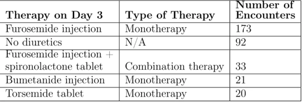
Table 3.7: Most common diuretic treatments for day 3 in dataset 1 Therapy on Day 3 Type of Therapy

Number of Encounters Furosemide injection Monotherapy 173

No diuretics N/A 92

Furosemide injection +

spironolactone tablet Combination therapy 33 Bumetanide injection Monotherapy 21 Torsemide tablet Monotherapy 20

Moreover, optimal values may correspond to some combinations that are not used in clinical practice. To address this problem, we only considered diuretic regimens that are most commonly used to treat patients admitted with a CHF exacerbation; i.e., we restricted the space of potential therapies to those that were prescribed in at least 20 encounters in Dataset 1. Therapies given in at least 20 encounters on the third day are shown in Table 3.7.

To search over all possible treatments and find the optimal therapy on day 3, a zero dose was assigned to every diuretic on day 3 except for the diuretic(s) in consideration, whose dose(s) was varied between 0 and 1 (max dose) with a step-size of 0.02. An alternate method for diuretic optimization is discussed in Appendix B.

The results of the optimization are shown in Figure 3-3. There was a mean increase in P(desired outcome) for all three outcomes. The mean increase represents the gain in probability of achieving the desired outcome from choosing the optimal treatment decision on day 3. The biggest increase occurred in the creatinine outcome (+0.024), while the smallest increase occurred in the combined outcome (+0.007).

To evaluate the treatment decisions made by the algorithm, we computed the Euclidean distance between the optimal regimen and the actual regimen for each encounter in Dataset 2 (Equation 3.1). For an encounter, the Euclidean distance between the optimal regimen and the actual regimen was calculated as:

𝐷( ⃗𝑜𝑝𝑡, ⃗𝑎𝑐𝑡) = ⎯ ⎸ ⎸ ⎷ 𝐿 ∑︁ 𝑑=1 ( ⃗𝑜𝑝𝑡[𝑑] − ⃗𝑎𝑐𝑡[𝑑])2 _(3.1)

Figure 3-3: Optimization results for weight (A), creatinine (B), and combined (C) outcomes

where 𝐿 = 21 is the total number of diuretics, ⃗𝑜𝑝𝑡 is a vector containing the diuretic doses in the optimal regimen, and ⃗𝑎𝑐𝑡 is a vector containing the diuretic doses in the actual regimen. If more than one regimen was deemed optimal, the regimen closest to the actual regimen was used. Distances were divided into three classes, low (𝐷( ⃗𝑜𝑝𝑡, ⃗𝑎𝑐𝑡) = 0), medium (0 < 𝐷( ⃗𝑜𝑝𝑡, ⃗𝑎𝑐𝑡) < 1) and high (𝐷( ⃗𝑜𝑝𝑡, ⃗𝑎𝑐𝑡) ≥ 1). The probability of having a desired outcome (the fraction of encounters with a desired outcome) was computed for each distance class.

An evaluation of the diuretic optimization is shown in Figure 3-4. The probabil-ity of a desired creatinine outcome was highest (p=0.79) in the class of encounters whose diuretic regimens were closest to an optimal regimen (low distance), and low-est (p=0.45) in the class of encounters whose regimens deviated the most from an optimal regimen (high distance). A similar trend exists for the combined outcome: encounters most similar to an optimal regimen had the highest probability of a desired outcome (p=0.33), and those least similar to an optimal regimen had the lowest prob-ability of a desired outcome (p=0.18). For the weight outcome, encounters closest to an optimal regimen had the highest probability (p=0.50) of achieving their desired weight. However, encounters with a high distance from an optimal regimen had a slightly greater probability (p=0.19) of achieving their desired weight compared to encounters with a medium distance (p=0.14).

Figure 3-4: Evaluation of optimization results for creatinine, weight, and combined outcomes; distance refers to the Euclidean distance between the optimal and actual diuretic regimens

Chapter 4

Summary and Conclusions

4.1

Conclusions

Dynamic treatment regimens have wide applications in a variety of clinical settings, including sepsis, cancer, and HIV trials. This thesis focuses on the application of DTRs to arrive at personalized diuretic treatment regimens for CHF patients.

In this work, we constructed a dataset of 679 encounters with an admitting di-agnosis of CHF. The feature set included demographics, medical histories, comorbid diseases, vital signs, laboratory results, medications, and clinical outcomes. By train-ing an artificial neural network on these data, we were able to predict outcomes at discharge related to volume status and kidney function with an AUC of 0.77-0.80. We also characterized diuretic therapies given to patients in the dataset to curate a set of possible diuretic treatments. Lastly, we used our trained models to optimize the treatment decision on the third day. For two outcomes of interest, we showed that a smaller difference between the actual and optimal regimen correlated with a higher probability of achieving a desired outcome after 5 days or at discharge. The results suggest that data available in the electronic medical record (EMR) can be used to predict clinical outcomes of interest and generate treatment regimens in CHF patients. However, it is important to note that this work only optimized diuretics on the third day of stay.

the goal of enhancing patient outcomes. As such, our future vision is the integration of these methods with the EMR. Upon admission, a patient’s real-time data would be fed into the model. Taking into consideration a host of clinical variables, the model would recommend an individualized, responsive treatment regimen designed to optimize their clinical outcomes. Our aim is to aid, not replace, clinicians with the model’s data-driven decisions.

4.2

Limitations and Future Directions

There are a few limitations of this work that should be addressed. Firstly, the pa-tients in Dataset 1 and Dataset 2 were treated at a single academic teaching hospital. Thus, we are unable to show that our models generalize across patient populations. Incorporating different patient and provider populations would help to improve ro-bustness. Augmenting the number of patients in the dataset would likely also increase the model’s performance. However, the use of healthcare data for research purposes must be balanced with patient privacy, and challenges in data access remain.

Secondly, our dataset lacks certain features that are important for tailoring di-uretic regimens. One example of a missing feature is the ejection fraction (EF). The EF exists in the EMR as an unstructured field that we were unable to obtain due to resource limitations. Other missing variables, such as ethnicity and socioeconomic status (SES), relate to patient demographics. Since HF risk factors, prognosis, and management guidelines differ across ethnicities and SES [18], these may be worth-while fields to include. Enriching the dataset with these features may help to improve the predictive power of the models and adjust for biases. However, increasing the number of features may necessitate some method of feature selection (i.e. least ab-solute shrinkage and selection operator) and/or regularization (i.e. L2 regularization

or Dropout). With the addition of more features, imputation may also be needed to address the problem of missing data. Common imputation methods are mean substitution and multivariate normal imputation.

represent the full spectrum of possible therapies that can be prescribed. Limiting the action space may have resulted in a suboptimal treatment decisions.

Additional outcomes of interest, depending on the use case, can also be considered. A more complex model could be trained to incorporate multiple, long-term outcomes - for example, length of hospital stay, mortality, readmission, and adverse events. The existing model only optimizes for short-term outcomes (i.e. volume and renal status at discharge); future models could also optimize for the long-term health of the patient. Cost and hospital resource utilization may also be considered.

Lastly, this thesis focused on optimizing the treatment decision for a single day, and the bulk of the remaining work lies in constructing full-length DTRs. In addition, there remain opportunities to extend the length of the regimen and/or increase the frequency of treatment intervals.

Chapter 5

Methods

5.1

Dataset Curation and Preprocessing

A total of 679 CHF encounters at Massachusetts General Hospital were included in the cohort: 617 encounters in Dataset 1 and 63 encounters in Dataset 2. The ranges of admission dates for patients in Dataset 1 and Dataset 2 were April 2016 - October 2018 and June 2018 - September 2019, respectively. Data in the Epic electronic medical record (EMR) system were stored in a secondary database called the Clinical Dataset Animination Center (CDAC). The CDAC data were mined using SQL and processed using Python.

5.1.1

Admitting Diagnosis and Comorbid Diseases

Encounters were only included in Datasets 1 and 2 if the admission diagnosis con-tained any of the following strings: "heart fail," "chf," "hrt fail," "right ventricular failure," "rvf," "congestive cardiac failure," "lvr," and "left ventricular failure." Each encounter was manually inspected to ensure a primary admitting diagnosis of heart failure.

Patients were labeled with a prior diagnosis of CKD if they had any previous diagnosis containing "ckd," "kidney disease," "renal insufficiency," "renal failure," or “renal azotemia.” Patients were labeled with a prior diagnosis of COPD if they

had any previous diagnosis containing "copd," "chronic obstructive pulmonary dis-ease," "chronic pulmonary disdis-ease," "bronchitis," "emphysema," "respiratory fail-ure," or "chronic pulmonary disease." Patients with a prior diagnosis of "bronchitis" or "respiratory failure" were only labeled with COPD if the prior diagnosis contained "chronic" and not "acute." Patients were labeled with a smoking diagnosis if they had any previous diagnosis containing "smok," "nicotine," or "tobacco."

5.1.2

Feature Selection

We sought to choose a feature set that would balance the dataset size with feature richness. Daily values for weight and serum creatinine formed the initial inclusion criteria. Considering all encounters with a daily weight and serum creatinine, we selected features that were present for all three days in 95% of the encounters. Lab-oratory results whose values were indeterminate (i.e. "1+," "2+," "3+," "negative," "cancelled," "refused," "credit", "unable to report urine chemistry results," "quantity not sufficient") were excluded. By this method, we chose potassium, glucose, calcium, sodium, anion gap, chloride, BUN, and CO2 as the additional features.

All medications prescribed in any of the encounters in Dataset 1 were considered as potential features. However, only those which passed two criteria were included in the final feature set. Firstly, the medication had to be administered at a nonzero dose in the first three days of at least one encounter. Secondly, the medication had to be confirmed (by a cardiologist) as a heart failure medication or diuretic.

5.1.3

Preprocessing Pipeline

The sequence of inclusion criteria used to filter the CDAC dataset is described below. Only encounters that met all of the criteria were included in Datasets 1 and 2.

1. Inpatient encounters where the admitting diagnosis included any of ("heart fail," "chf," "hrt fail," "right ventricular failure," "rvf," "congestive cardiac failure," "lvf," "left ventricular failure") and passed a manual inspection test

3. LOS ≥ 3 days

4. Included at least one serum creatinine level prior to admission 5. Included a dry weight estimate ≤ weight upon admission 6. Included a NT-ProBNP upon admission

7. Included full weight data for the first three days, where 22 kg < weight < 350 kg for each weight (to exclude pediatric cases and typography errors)

8. Included full serum creatinine data for the first three days

9. Included full data for the remaining laboratory values (potassium, glucose, cal-cium, sodium, anion gap, chloride, BUN, and CO2) for the first three days

The pipeline for Datasets 1 and 2 are shown in Figures 5-1A and 5-1B, respectively. The bottleneck in Dataset 2 is a result of missing data; laboratory data for that cohort only extend back to April 2018. Thus, many of them lack a serum creatinine level prior to admission.

5.2

Machine Learning Methods

5.2.1

Artificial Neural Networks

Artificial neural networks (ANNs) are a type of supervised learning method, in which a function is learned from known input-output pairs. Their architecture is modeled after the neuronal connections of the brain. ANNs consist of nodes ("neurons") that are linked by connections, each of which has an associated weight. These nodes are organized into different layers: an input layer, output layer, and hidden layers in between.

The simplest type of ANN is called a feedforward neural network. In feedforward neural networks, the nodes in each layer are connected to the next layer, so that information only travels forward from the input to the output layer without going

Figure 5-1: Pipeline for dataset 1 (A) and dataset 2 (B)

through cycles. If each node in a layer is connected to every node in the previous layer, the layer is considered fully-connected (FC). Figure 5-2 shows a small feedforward neural network with 3 input nodes, one hidden layer with 2 nodes, and 1 input. The output of the nodes in the hidden and output layers are functions of the sum of the weighted outputs of the nodes in the previous layer. These functions are known as activation functions and are used to introduce nonlinearities to the network. Common activations functions include ReLU, Sigmoid, and Tanh. The training process of a neural network involves iterative updates to the weights via the backpropagation algorithm until the model converges to an optimal solution.

5.2.2

Recurrent Neural Networks

Recurrent neural networks (RNNs) are a type of ANN that takes advantage of the sequential information present in data. RNNs have been used successfully in tasks such as sequence prediction, sentiment classification, and machine translation. Unlike feedforward neural networks, RNNs have connections which form a directed cycle.

Figure 5-2: Feedforward neural network

Figure 5-3: Recurrent neural network schematic

This enables intermediate outputs from previous steps to be fed as inputs into the current step, so that an internal memory is preserved as hidden states. Figure 5-3 shows an RNN with 𝑘 time-steps that has been unrolled. Here, 𝑋 is the input, 𝑌 represents the output, and 𝐻 represents an RNN cell. In the unrolled version, 𝑋1 is

input into 𝐻1, which outputs an intermediate output 𝑌1. Both 𝑌1 and 𝑋2 are input

into the next RNN cell, 𝐻2, which outputs 𝑌2, and so on until the final output 𝑌𝑘 is

produced. In this way, the RNN "remembers" information from previous time-steps during the learning process, which provides a suitable model for the time series data we use in this work.

The neural network trained in this work is shown in Figure 5-4, with variable descriptions and dimensions presented in Table 5.1. The model comprises an RNN connected to a feedforward network. The reasoning behind this architecture lies in the

temporal nature of the data processed by the RNN. ReLU activations are applied to the hidden layers in the RNN to introduce nonlinearities. The number of hidden layers in the RNN is varied between 2 and 3. The time-invariant covariates are merged with the output of the RNN to form a 10-unit vector. A FC layer with a ReLU activation function allows for nonlinear interactions between the output of the RNN and the covariates. Finally, the sigmoid function is applied to the output of the FC layer to produce an output representing the probability that a given encounter achieves a desired outcome. The sigmoid function ensures that the output is a number between 0 and 1, and is defined as follows:

𝜎(𝑥) = 1

1 + 𝑒−𝑥 (5.1)

where 𝑥 is the weighted sum of the nodes from the previous layer.

The neural network was trained using the Adam optimizer, with binary cross-entropy as the loss function. Cross-cross-entropy is commonly used as the loss function in classification problems, and is defined for the binary case as

𝐶𝐸(𝑦, ˆ𝑦) = −1 𝑁 𝑁 ∑︁ 𝑛=1 𝑦𝑛· 𝑙𝑜𝑔( ˆ𝑦𝑛) + (1 − 𝑦𝑛) · 𝑙𝑜𝑔(1 − ˆ𝑦𝑛) (5.2)

where 𝑦𝑛 is the true class label and ˆ𝑦𝑛 is the predicted probability of the class

label for encounter 𝑛.

The hyperparameter space was sweeped using the grid searches presented in Tables 5.2 and 5.3. The validation loss was monitored and early-stopping was applied with a patience parameter of 100. All code for the neural network models was written in Python 3 using Keras.

Figure 5-4: Neural network model architecture

Table 5.1: Neural network variable descriptions and dimensions Variable Description Dimensions 𝑋𝑗 Inputs on day 𝑗 1 × 55

𝑌𝑗 Intermediate output for day 𝑗 Scalar

𝑊𝑥,𝑗 Weights for day 𝑗 inputs 55 × ℎ

𝑊𝑦,𝑗 Weights for day 𝑗 − 1 output 1 × ℎ

Covariates 9 covariates 1 × 9 ℎ Number of nodes in the recurrent hidden layer Scalar

Table 5.2: Grid search for neural network with 2 hidden layers in the RNN Hyperparameter Values

Learning rate [0.1,0.01,0.005,0.001,0.0005,0.0001] Batch size [32,64,128]

Nodes in recurrent layer 1 [16,20,24,28,32] Nodes in recurrent layer 2 [12,16,20,24,28] Nodes in fully-connected layer [10,14,18,22]

Table 5.3: Grid search for neural network with 3 hidden layers in the RNN Hyperparameter Values

Learning rate [0.1,0.01,0.005,0.001,0.0005,0.0001] Batch size [32,64,128]

Nodes in recurrent layer 1 [16,20,24,28,32] Nodes in recurrent layer 2 [12,16,20,24,28] Nodes in recurrent layer 2 [8,12,16,20,24] Nodes in fully-connected layer [10,14,18,22]

Appendix A

Previous Prediction Tasks and

Q-Functions

Initial models aimed to predict patients’ length of stay (LOS) in the hospital, mod-eled as a regression problem. Both linear regression and neural network models were trained and optimized to predict LOS. However, we found that the current dataset and models were not able to predict LOS with sufficient accuracy. We then bina-rized LOS into short (fewer than 5 days) and long (greater than or equal to 5 days) admissions; we were able to predict LOS class with moderate success using a neural network. We also introduced the three clinical outcomes (discharge weight, discharge creatinine, and discharge weight + creatinine) and found more success in classifying these compared to LOS. We theorized that the information present in our feature set, which mainly comprises clinical variables and medications, is more directly related to weight and creatinine than to LOS.

Appendix B

Additional Method for Diuretic

Optimization

An alternate approach was taken to perform the diuretic optimizations. In this ap-proach, only the dose of the diuretic(s) in consideration was varied between 0 and 1 (max dose) with a step-size of 0.02. None of the other diuretic doses were modified.

The results of the optimization without zeroing out diuretics are shown in Fig-ure B-1. There was a mean increase in P(desired outcome) for all three outcomes. The biggest increase occurred for the creatinine outcome (+0.010), and the smallest increase occurred for the combined outcome (+0.004).

The evaluation for the diuretic optimization without zeroing out diuretics is shown in Figure B-2. The probability of a desired creatinine outcome was highest in the low and medium distance classes. However, the other data indicate that the optimization did not work as expected. For example, for the weight and combined outcomes, the highest probability of a desired outcome occurred in the medium distance class - not in the low distance class. Moreover, for the combined outcome, the probability of a desired outcome was greater in the high distance class than in the low distance class.

Figure B-1: Optimization results (without zeroing out diuretics) for creatinine, weight, and combined outcomes

Figure B-2: Evaluation of optimization results (without zeroing out diuretics) for creatinine, weight, and combined outcomes; distance refers to the Euclidean distance between the optimal and actual diuretic regimens

Bibliography

[1] D. Chambers, C. Huang, and G. Matthews, Basic Physiology for Anaesthetists. Cambridge, England: Cambridge University Press, 2015.

[2] M. Olofsson, H. Jansson, and K. Boman, “Predictors for hospitalizations in el-derly patients with clinical symptoms of heart failure: A 10-year observational primary healthcare study,” Journal of Clinical Gerontology and Geriatrics, vol. 7, no. 2, pp. 53–59, 2016.

[3] M. Konstam, “Heart failure costs, minority populations, and outcomes: Tar-geting health status, not utilization, to bend the cost-effectiveness curve,” Journal of the American College of Cardiology, vol. 6, no. 5, pp. 398–400, 2018. [4] S. Hollenberg, L. Stevenson, T. Ahmad, V. Amin, J. B. Biykem Bozkurt, L. Davis, M. Drazner, J. Kirkpatrick, P. Peterson, B. Reed, C. Roy, and A. Stor-row, “2019 ACC expert consensus decision pathway on risk assessment, man-agement, and clinical trajectory of patients hospitalized with heart failure,” Journal of the American College of Cardiology, vol. 74, no. 15, pp. 1966–2011, 2019.

[5] M. Figueroa and J. Peters, “Congestive heart failure: Diagnosis, pathophysiology, therapy, and implications for respiratory care,” Respiratory Care, vol. 51, no. 4, pp. 403–412, 2006.

[6] A. Shah, D. Gandhi, S. Srivastava, K. Shah, and R. Mansukhani, “Heart failure: A class review of pharmacotherapy,” Pharmacy and Therapeutics, vol. 42, no. 7, pp. 464–472, 2017.

[7] H. Shahbaz and M. Gupta, “Creatinine clearance,” StatPearls, 2019.

[8] A. Ahmed and R. Campbell, “Epidemiology of chronic kidney disease in heart failure,” Heart Failure Clinics, vol. 4, no. 4, pp. 387–399, 2008.

[9] Y. Liu, D. Zeng, and Y. Wang, “Use of personalized dynamic treatment regimes (DTRs) and sequential multiple assignment randomized trials (SMARTs) in men-tal health studies,” Shanghai Archives of Psychiatry, vol. 26, no. 6, pp. 376–383, 2014.

[10] L. Wang, A. Rotnitzky, X. Lin, R. Millikan, and P. Thall, “Evaluation of viable dynamic treatment regimes in a sequentially randomized trial of advanced prostate cancer,” Journal of the American Statistical Association, vol. 107, no. 498, pp. 493–508, 2012.

[11] M. Komorowski, L. Celi, O. Badawi, A. Gordon, and A. A. Faisal, “The artificial intelligence clinician learns optimal treatment strategies for sepsis in intensive care,” Nature Medicine, vol. 24, no. 11, pp. 1716–1720, 2018.

[12] R. Sutton and A. Barto, Reinforcement Learning: An Introduction. Cambridge, Massachusetts: The MIT Press, 2nd ed., 2018.

[13] S. Murphy, “A generalization error for Q-learning,” Journal of Machine Learning Research, vol. 6, pp. 1073–1097, 2005.

[14] E. Moodie, B. Chakraborty, and M. Kramer, “Q-learning for es-timating optimal dynamic treatment rules from observational data,” Canadian Journal of Statistics, vol. 40, no. 4, pp. 629–645, 2012.

[15] P. Lavori, R. Dawson, and A. J. Rush, “Flexible treatment strategies in chronic disease: Clinical and research implications,” Biological Psychiatry, vol. 48, pp. 605–614, 2000.

[16] P. Lavori and R. Dawson, “Dynamic treatment regimes: practical design consid-erations,” Clinical Trials, vol. 1, no. 1, pp. 9–20, 2004.

[17] P. Wright and M. Thomas, “Pathophysiology and management of heart failure,” Clinical Pharmacist, vol. 10, no. 12, 2018.

[18] N. Downing, C. Wang, and A. Gupta, “Association of racial and socioeconomic disparities with outcomes among patients hospitalized with acute myocardial infarction, heart failure, and pneumonia an analysis of within- and between-hospital variation,” JAMA Network Open, vol. 1, no. 5, 2018.