Distinct Cortical Pathways for Music and Speech Revealed by Hypothesis-Free Voxel Decomposition

(1)

Distinct Cortical Pathways for Music and Speech

Revealed by Hypothesis-Free Voxel Decomposition

The MIT Faculty has made this article openly available.

Please share

how this access benefits you. Your story matters.

Citation

Norman-Haignere, et al. “Distinct Cortical Pathways for Music and

Speech Revealed by Hypothesis-Free Voxel Decomposition.” Neuron

88, 6 (December 2015): 1281–1296 © 2015 Elsevier

As Published

http://dx.doi.org/10.1016/J.NEURON.2015.11.035

Publisher

Elsevier/Cell Press

Version

Author's final manuscript

Citable link

http://hdl.handle.net/1721.1/112175

Terms of Use

Creative Commons Attribution-NonCommercial-NoDerivs License

(2)

Distinct Cortical Pathways for Music and Speech Revealed by

Hypothesis-Free Voxel Decomposition

Sam Norman-Haignere1,*, Nancy G. Kanwisher#1,2, and Josh H. McDermott#1 1_{Department of Brain and Cognitive Sciences, MIT}

2_{McGovern Institute for Brain Science, MIT}

#_{These authors contributed equally to this work.}

SUMMARY

The organization of human auditory cortex remains unresolved, due in part to the small stimulus sets common to fMRI studies and the overlap of neural populations within voxels. To address these challenges, we measured fMRI responses to 165 natural sounds and inferred canonical response profiles (“components”) whose weighted combinations explained voxel responses throughout auditory cortex. This analysis revealed six components, each with interpretable response characteristics despite being unconstrained by prior functional hypotheses. Four components embodied selectivity for particular acoustic features (frequency, spectrotemporal modulation, pitch). Two others exhibited pronounced selectivity for music and speech, respectively, and were not explainable by standard acoustic features. Anatomically, music and speech selectivity concentrated in distinct regions of non-primary auditory cortex. However, music selectivity was weak in raw voxel responses, and its detection required a decomposition method. Voxel decomposition identifies primary dimensions of response variation across natural sounds, revealing distinct cortical pathways for music and speech.

INTRODUCTION

Just by listening, humans can discern a vast array of information about the objects and events in the environment around them. This ability to derive information from sound is instantiated in a cascade of neuronal processing stages extending from the cochlea to the auditory cortex. Although much is known about the transduction and subcortical processing of sound, cortical representations of sound are less well understood. Prior work has revealed tuning in and around primary auditory cortex for acoustic features such as frequency (Costa et al., 2011; Humphries et al., 2010), temporal and spectral modulations (Barton et al., 2012; Chi et al., 2005; Santoro et al., 2014; Schönwiesner and Zatorre, 2009), spatial cues

(Rauschecker and Tian, 2000; Stecker et al., 2005), and pitch (Bendor and Wang, 2005; Norman-Haignere et al., 2013; Patterson et al., 2002). The tuning properties of non-primary

*_{Correspondence: snormanhaignere@gmail.com.}

Publisher's Disclaimer: This is a PDF file of an unedited manuscript that has been accepted for publication. As a service to our

customers we are providing this early version of the manuscript. The manuscript will undergo copyediting, typesetting, and review of

HHS Public Access

Author manuscript

Neuron. Author manuscript; available in PMC 2016 December 16.

Published in final edited form as:

Neuron. 2015 December 16; 88(6): 1281–1296. doi:10.1016/j.neuron.2015.11.035.

Author Manuscript

(3)

regions are less clear. Although many studies have reported selectivity for vocal sounds (Belin et al., 2000; Petkov et al., 2008) and speech (Mesgarani et al., 2014; Overath et al., 2015; Scott et al., 2000), the cortical representation of environmental sounds (Engel et al., 2009; Giordano et al., 2012) and of music (Abrams et al., 2011; Angulo-Perkins et al., 2014; Fedorenko et al., 2012; Koelsch et al., 2005; Leaver and Rauschecker, 2010; Rogalsky et al., 2011; Tierney et al., 2013) is poorly understood. Moreover, debate continues about the extent to which the processing of music, speech, and other natural sounds relies on shared vs. distinct neuronal mechanisms (Peretz et al., 2015; Zatorre et al., 2002), and the extent to which these mechanisms are organized hierarchically (Chevillet et al., 2011; Hickok and Poeppel, 2007; Staeren et al., 2009).

This paper was motivated by two limitations of many neuroimaging studies (including our own) that have plausibly hindered the understanding of human auditory cortical

organization. First, responses are typically measured to only a small number of stimulus dimensions chosen to test particular hypotheses. Because there are many dimensions to which neurons could be tuned, it is difficult to test the specificity of tuning, and to know whether the dimensions tested are those most important to the cortical response. Second, the spatial resolution of fMRI is coarse: each voxel represents the aggregate response of hundreds of thousands of neurons. If different neural populations spatially overlap, their response will be difficult to isolate using standard voxel-wise analyses.

To overcome these limitations, we developed an alternative method for inferring neuronal stimulus selectivity and its anatomical organization from fMRI data. Our approach tries to explain the response of each voxel to a large collection of natural sounds as the weighted sum of a small number of response profiles (“components”), each potentially reflecting the tuning properties of a different neuronal sub-population. This method discovers response dimensions from structure in the data, rather than testing particular features hypothesized to drive neural responses. And unlike standard voxel-wise analyses, our method can isolate responses from overlapping neural populations, because multiple response profiles are used to model each voxel. When applied to auditory cortex, voxel decomposition identifies a small number of interpretable response dimensions, and reveals their anatomical organization in the cortex.

RESULTS

Experiment I: Modeling Voxel Responses to Commonly Heard Natural Sounds

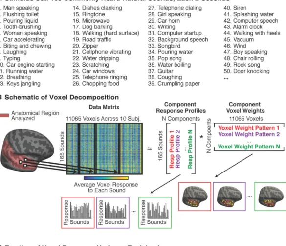
We measured the average response of voxels throughout auditory cortex to a diverse collection of 165 natural sounds (Figure 1A). The sound set included many of the most frequently heard and recognizable sounds that humans regularly encounter. We modeled each voxel's response as the weighted combination of a set of “components” (Figure 1B). Each component was defined by a response profile across the 165 sounds, and a vector of weights across the voxels, specifying the contribution of that response profile to each voxel. Notably, no information about either the specific sounds or the anatomical positions of voxels was used to infer components. Thus, any consistent structure that emerges from the

Author Manuscript

(4)

Voxel Decomposition

The 165-dimensional response vectors from all voxels in all subjects were concatenated to form the data matrix (11,065 voxels across all ten subjects). To discover components, we searched for matrix factorizations that could approximate the data matrix as the product of two smaller matrices: a ‘response’ matrix and a ‘weight’ matrix (see Figure 1B). The response matrix expresses the response of each discovered component to each sound (165 sounds × N components), and the weight matrix expresses the contribution of each component to each voxel (N components × 11065 voxels).

For a given number of components, the factorization is not unique, and must be constrained by additional criteria. We constrained the factorization with assumptions about the

distribution of component weights across voxels. We took advantage of the fact that summing independent random variables tends to produce a quantity that is closer to Gaussian-distributed. Thus, if voxel responses are a weighted sum of components with non-Gaussian weight distributions across voxels, the components should be identifiable as those whose weight distributions deviate most from Gaussianity. We searched for components with non-Gaussian weight distributions using two different algorithms. The first algorithm, a variant of independent components analysis (Hyvarinen, 1999), quantified deviations from Gaussianity using a non-parametric measure of non-Gaussianity (‘negentropy’). The second algorithm used a non-Gaussian prior on the distribution of voxel weights (the Gamma distribution) and searched for response profiles that maximized the likelihood of the data given this prior. Both methods recovered components with non-Gaussian voxel weights that explained most of the reliable voxel response variance, providing empirical support for the assumption that the components underlying the data are distributed in a non-Gaussian manner. The specific response profiles and voxel weights discovered by each method were very similar, indicating that the results are robust to the specific statistical criterion used. We focus our discussion on the results of the first method because it is faster, more standard, and does not depend on a specific parameterization of the data.

The only free parameter in the analysis is the number of components. We found that six components were sufficient to explain more than 80% of the replicable voxel response variance (Figure 1C). Moreover, cross-validated prediction accuracy was best using just six components, indicating that components beyond the sixth were primarily driven by fMRI noise that did not replicate across scans (Figure S1). We focused on these first six components in all subsequent analyses.

We first describe the anatomical distribution of each component, obtained by projecting its voxel weights back into anatomical coordinates. We then describe the acoustic and semantic features of sounds that explained the response profile of each component. We refer to the components using numbers that reflect how much of their response could be accounted for by standard acoustic measures (1 being the most and 6 being the least, as explained below).

Component Voxel Weights Plotted in Anatomical Coordinates

We examined the component anatomy using group maps of the voxel weights. Maps were computed by aligning each subject to a standardized anatomical template, averaging the

Author Manuscript

(5)

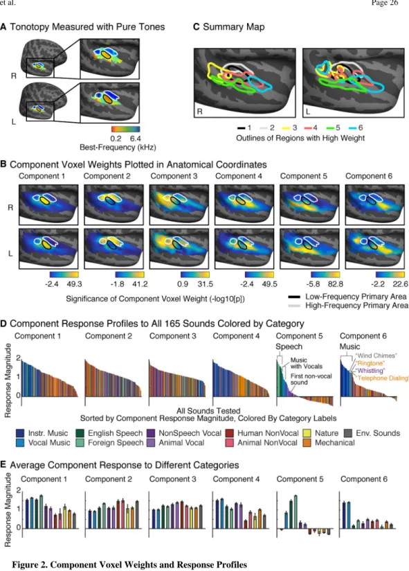
voxel weights for each component across subjects, and transforming this average weight into a measure of statistical significance (see Supplemental Methods). For comparison, we identified tonotopic gradients using responses to pure tones. A group tonotopic map exhibited the two mirror-symmetric gradients widely observed in primary auditory cortex (Figure 2A) (Humphries et al., 2010). Figure 2B plots component weight maps with outlines of high- and low-frequency primary fields overlaid (see Figure S2 for weight maps from the parametric model). Tonotopic maps and voxel weights from individual subjects were generally consistent with the group results (Figure S3). As a summary, Figure 2C plots outlines of the regions with highest weight for each component.

Although no anatomical information was used to infer components, voxel weights for each component were significantly correlated across subjects (p < 0.001; permutation test). The weights systematically varied in their overlap and proximity to primary auditory cortex (as defined tonotopically). Components 1 & 2 primarily explained responses in low- and high-frequency tonotopic fields of primary auditory cortex (PAC), respectively. Components 3 & 4 were localized to distinct regions near the border of PAC: concentrated anteriorly and posteriorly, respectively. Components 5 & 6 concentrated in distinct non-primary regions: Component 5 in the superior temporal gyrus, lateral to PAC, and Component 6 in the planum polare, anterior to PAC, as well as in the left planum temporale, posterior to PAC. All of the components had a largely bilateral distribution; there were no significant

hemispheric differences in the average weight for any of the components (Figure S4). There was a non-significant trend for greater weights in the left hemisphere of Component 6 (t(9) = 2.21; p = 0.055), consistent with the left-lateralized posterior region evident in the group map.

Component Response Profiles and Selectivity for Sound Categories

Figure 2D plots the full response profile of each discovered component to each of the 165 tested sounds. Sounds are colored based on their membership in one of 11 different categories. These profiles were reliable across independent fMRI scans (test-retest correlation: r = 0.94, 0.88, 0.70, 0.93, 0.98, 0.92 for Components 1-6, respectively; Figure S5A). The response profiles were also relatively robust to the exact sounds tested (Figure S5B): for randomly subsampled sets of 100 sounds, the profiles discovered were highly correlated with those discovered using all 165 sounds (median correlation >0.95 across subsampled sound sets for all 6 components).

Figure 2E plots the average response of each component to sounds with the same category label (assigned based on an online survey; see Methods). Components 1-4 responded substantially to all of the sound categories. In contrast, Components 5 and 6 responded selectively to sounds categorized as speech and music, respectively. Category labels accounted for more than 80% of the explainable response variance in these two components. For Component 5, all of the sounds that produced a high response were categorized as “English Speech” or “Foreign Speech”, with the next-highest response category being vocal

Author Manuscript

(6)

substantially lower than the response to speech. Notably, responses to foreign speech were at least as high as responses to English speech, even though all of the participants were native English speakers (this remained true after excluding responses to foreign languages that subjects had studied for at least 1 year). Component 5 thus responded selectively to sounds with speech structure, regardless of whether the speech conveyed linguistic meaning. Component 6, in contrast, responded primarily to sounds categorized as music: of the 30 sounds with the highest response, all but two were categorized as musical sounds by participants. Even the two exceptions were melodic: “wind chimes” and “ringtone” (categorized as “environmental” and a “mechanical” sounds respectively). Other non-musical sounds produced a low response, even those with pitch (e.g. speech).

The anatomical distribution of these components (Figure 2B) suggests that speech-and music-selective responses are concentrated in distinct regions of non-primary auditory cortex, with speech selectivity lateral to primary auditory cortex, and music selectivity anterior and posterior to primary auditory cortex. We emphasize that these components were determined by statistical criteria alone – no information about sound category or anatomical position contributed to their discovery. These results provide evidence that auditory cortex contains distinct anatomical pathways for the analysis of music and speech.

Response Correlations with Acoustic Measures

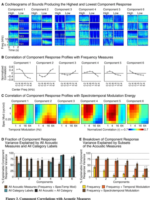
We next explored the acoustic sensitivity of each component, both to better understand their response properties, and to test whether the selectivity of Components 5 and 6 for speech and music could be explained by standard acoustic features. First, we visualized the acoustic structure of the sounds that produced the highest and lowest response for each component by plotting their “cochleograms” – time-frequency decompositions, similar to spectrograms, intended to summarize the cochlea's representation of sound (Figure 3A). We then computed the correlation of each component's response profile with acoustic measures of frequency and spectrotemporal modulation for each sound (Figures 3B and 3C).

These analyses revealed that some of the components could be largely explained by standard acoustic features. Component 1 produced a high response for sounds with substantial low-frequency energy (Figure 3A&B; p<0.001, permutation test), consistent with the anatomical distribution of its voxel weights, which concentrated in the low-frequency field of PAC (Figure 2B). Conversely, Component 2 responded preferentially to sounds with high-frequency energy (p < 0.001), and overlapped the high-high-frequency fields of PAC. This result demonstrates that our method can discover a well-established feature of auditory cortical organization.

Components 3 and 4 were primarily selective for patterns of spectrotemporal modulation in the cochleograms for each sound. The sounds eliciting the highest response in Component 3 were composed of broadband events that were rapidly modulated in time, evident as vertical streaks in the cochleograms. In contrast, the sounds eliciting the highest response in

Component 4 all contained pitch, evident in the cochleograms as horizontal stripes, or spectral modulations, reflecting harmonics. The contrast between these two components is suggestive of a tradeoff in sensitivity to spectral vs temporal modulations (Singh and

Author Manuscript

(7)

Theunissen, 2003). Accordingly, the response profile of Component 3 correlated most with measures of fast temporal modulation and coarse-scale spectral modulation (p < 0.01), while that of Component 4 correlated with measures of fine spectral modulation and slow temporal modulation (p < 0.001) (Figure 3C). We also observed significant modulation tuning in Components 1 and 2 (for fine spectral and rapid temporal modulations, respectively; p < 0.001), beyond that explained by their frequency tuning (frequency measures were partialled out before computing the modulation correlations).

Prior studies have argued that the right and left hemispheres are differentially specialized for spectral and temporal resolution, respectively (Zatorre et al., 2002). Contrary to this

hypothesis, Components 1-4 exhibited qualitatively similar patterns of voxel weights in the two hemispheres (Figure 2B), with no significant hemispheric differences when tested individually. However, the small biases present were in the expected direction (Figure S4), with a right-hemisphere bias for Components 1 & 4, and a left-hemisphere bias for Components 2 & 3. When these laterality differences (RH-LH) were pooled and directly compared ([C1 + C4] – [C2 + C3]), a significant difference emerged (t(9) = 2.47; p < 0.05). These results are consistent with the presence of hemispheric biases in spectral and temporal modulation sensitivity, but show that this bias is quite small relative to within-hemisphere differences.

Collectively, measures of frequency and modulation energy accounted for much of the response variance in Components 1-4 (Figure 3D; 86%, 76%, 68%, and 67% respectively; see Figure 3E for the variance explained by subsets of acoustic measures). Category labels explained little to no additional variance for these components. In contrast, for Components 5 and 6, category labels explained substantially more variance than the acoustic features (p < 0.001), and when combined, acoustic features explained little additional variance beyond that explained by the categories. Thus, the selectivity of Components 5 and 6 for speech and music sounds cannot be explained by standard acoustic features.

Experiment II: Speech and Music Scrambling

Music and speech are both notable for having distinct and recognizable structure over relatively long time scales. One approach to probing sensitivity to temporal structure is to reorder short sound segments so that local but not global structure is preserved (Abrams et al., 2011). A recent study introduced “quilting” for this purpose – a method for reordering sound segments while minimizing acoustic artifacts (Overath et al., 2015) – and

demonstrated that regions in the superior temporal gyrus respond preferentially to intact compared with quilt-scrambled speech. We used the same procedure to provide an additional test of the selectivity of our components.

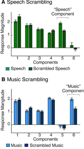
We measured responses to intact and scrambled speech and music in the same subjects scanned in Experiment I. As a result, we could use the component voxel weights from Experiment I to infer the response of each component to the new stimulus conditions from Experiment II. For Components 1-4, there was little difference in response to the intact and scrambled sounds for either category (Figures 4A&B). In contrast, Component 5 responded

Author Manuscript

(8)

between category (speech, music), scrambling, and components (F(1,5) = 7.37, p < 0.001). This result provides further evidence that Components 5 and 6 respond selectively to speech and music structure, respectively.

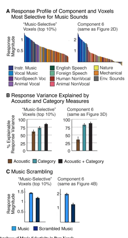
Searching for Music-Selective Responses with Standard Methods

There are few prior reports of highly selective responses to musical sounds (Angulo-Perkins et al., 2014; Leaver and Rauschecker, 2010). One possible explanation is that prior studies have tested for music selectivity in raw voxel responses. If music-selective neural

populations overlap within voxels with other neural populations, the music-selectivity of raw voxel responses could be diluted. Component analysis should be less vulnerable to such overlap because voxels are modeled as the weighted sum of multiple components. To test this possibility, we directly compared the response of the music-selective component (Component 6) with the response of the voxels most selective for music (Figure 5) (see Methods). We found that the selectivity of these voxels for musical structure was notably weaker than that observed for the music-selective component across a number of metrics. First, the response profiles to the sound set were graded for the voxels but closer to binary for the component (i.e., high for music, low for non-music) (Figure 5A). Second, acoustic features and category labels explained similar amounts of response variance in music-selective voxels, but category labels explained a much higher fraction of the component's response (Figure 5B). Third, although music-selective voxels responded slightly less to scrambled music (Figure 5C; t(7) = 4.82, p < 0.01), the effect was much larger in

Component 6, producing a significant interaction between the effect of scrambling (intact vs. scrambled) and the type of response being measured (component vs. voxel) (p < 0.01). The ability to decompose voxel responses into their underlying components was thus critical to identifying neural selectivity for music.

We observed similar but less pronounced trends when comparing speech-selective voxels with the speech-selective component (Component 5): speech-selective voxels exhibited robust selectivity for speech sounds (Figure S6) that could not be accounted for by standard acoustic features. This finding suggests that speech-selectivity is more anatomically segregated than music-selectivity, and thus easier to identify in raw voxel responses.

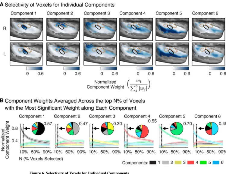
Selectivity of Voxels for Individual Components

The lack of clear music selectivity in raw voxels suggests that at least some components spatially overlap. We performed two analyses to quantify the extent of overlap between components. First, we assessed the selectivity of voxels for individual components (Figure 6A): for each voxel the weight for a single component was normalized by the sum of the absolute values of the weights for all six components. Normalized weights near 1 indicate voxels that weight strongly on a single component. Figure 6B plots normalized weights averaged across the top N% of voxels with the most significant weight along each individual component (varying N; permutation test, see Methods). Independent data was used to select voxels in individual subjects and measure their component weights to avoid statistical bias/ circularity. As a summary, inset pie charts show normalized weights averaged across the top 10% of voxels.

Author Manuscript

(9)

The highest normalized weights were observed for Component 5 (speech-selective) in the superior temporal gyrus (Figure 6A), consistent with the robust speech-selectivity we observed in raw voxels (Figure S6). The top 10% of voxels with the most significant weight for Component 5 had an average normalized weight of 0.70 (Figure 6B), and thus most of their response was explained by Component 5 alone. By contrast, there were no voxels with similarly high normalized weights for Component 6 (music-selective), consistent with the weak music selectivity observed in raw voxels (Figure 5). The top 10% of voxels for Component 6 (average normalized weight of 0.49) also had substantial weight from Component 4 (normalized weight of 0.20; Figure 6B), which responded preferentially to sounds with pitch. This finding is consistent with the anatomical distribution of these components, both of which overlapped a region anterior to primary auditory cortex (Figure 2B).

Testing Assumptions of non-Gaussianity

Our voxel component analysis relied on assumptions about the distribution of weights across voxels to constrain the factorization of the data matrix. The key assumption of our approach is that these weight distributions are non-Gaussian. This assumption raises two questions: first, does the assumption hold for the voxel responses we analyzed, and second, what properties of cortical responses might give rise to non-Gaussian voxel weights?

To evaluate whether the non-Gaussian assumption was warranted for our data set, we relied on the fact that linear combinations of Gaussian variables remain Gaussian. As a

consequence, our method would only have been able to discover components with non-Gaussian voxel weights if the components that generated the data also had non-non-Gaussian weights. We thus tested whether the voxel weights for the inferred components were significantly non-Gaussian (evaluated in independent data).

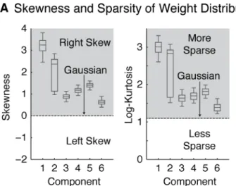
For all six components, the distribution of weights was significantly more skewed and kurtotic (sparse) than the Gaussian distribution (Figure 7A). As a result, a modified Gaussian distribution with flexible skew and sparsity (the 4-parameter ‘Johnson’

distribution) provided a significantly better fit to the weight distributions than the Gaussian (Figure 7B) (as measured by the log-likelihood of left-out data; p < 0.01 in all cases, via bootstrapping). These results show that all of the components discovered by our analysis are indeed non-Gaussian by virtue of being skewed and sparse, validating a key assumption underlying our approach (see also Figure S7).

Why would the distribution of neural selectivities in the brain be skewed and sparse? In practice, we found that the anatomical distributions of the component weights were spatially clustered. If neurons with similar response properties are spatially clustered in the brain, they should contribute substantially to only a small fraction of voxels, producing skewed and sparse weight distributions. Skew and sparsity may thus be useful statistical signatures for identifying components from fMRI responses, due to anatomical clustering of neurons with similar response selectivities.

Author Manuscript

(10)

DISCUSSION

Our findings reveal components of neuronal stimulus selectivity that collectively explain fMRI responses to natural sounds throughout human auditory cortex. Each component has a distinct response profile across natural sounds and a distinct spatial distribution across the cortex. Four components reflected selectivity for standard acoustic dimensions (Figure 3), such as frequency, pitch, and spectrotemporal modulation. Two other components were highly selective for speech and music (Figures 2D&E). The response of these two

components could not be explained by standard acoustic measures, and their specificity for speech and music was confirmed with hypothesis-driven experiments that probed sensitivity to category-specific temporal structure (Figure 4). The selective responses we observed for music have little precedent (Angulo-Perkins et al., 2014; Leaver and Rauschecker, 2010), and our analyses suggest an explanation: the music-selective component spatially

overlapped with other components (Figure 6). As a result, music-selectivity was not clearly evident in raw voxel responses, which are the focus of most fMRI analyses (Figure 5). Anatomically, the acoustically driven components (Components 1-4) concentrated in and around primary auditory cortex, whereas speech and music-selective components concentrated in distinct non-primary regions (Figure 2B). This pattern suggests that representations of music and speech diverge in non-primary areas of human auditory cortex. Our findings were enabled by a novel approach for discovering neural response dimensions (Figure 1). Our method searches the space of possible response profiles to natural stimuli for those that best explain voxel responses. The method is blind to the properties of each sound and the anatomical position of each voxel, but the components it discovers can be examined post-hoc to reveal tuning properties and functional organization. The method revealed both established properties of auditory cortical organization, such as tonotopy (Costa et al., 2011; Humphries et al., 2010), as well as novel properties not evident with standard methods.

Voxel Decomposition

Our method falls into a family of recent computational approaches that seek to uncover functional organization from responses to large sets of naturalistic stimuli. One prior approach has been to model voxel responses to natural stimuli using candidate sets of stimulus features (“encoding models”; Huth et al., 2012; Mitchell et al., 2008; Moerel et al., 2013). Such models can provide insights into the computations underlying neural activity, but require a prior hypothesis about the stimulus features encoded in voxel responses. Our approach is complementary: it searches for canonical response profiles to the stimulus set that collectively explain the response of many voxels, without requiring prior hypotheses about the stimulus features that underlie their response (Vul et al., 2012). While there is no guarantee that voxel responses will be explained by a small number of response profiles, or that the profiles will be interpretable, we found that auditory voxels could be explained by six components that each reflected selectivity for particular acoustic or semantic properties. An additional benefit of our approach is its ability to express voxel responses as the combination of distinct underlying components, potentially related to neural

sub-populations. We used linear decomposition techniques to discover components because the mapping between hemodynamic activity and the underlying neural response is thought to be

Author Manuscript

(11)

approximately linear (Boynton et al., 1996). Such techniques have previously been used to analyze fMRI timecourses (Beckmann and Smith, 2004), typically to reveal large-scale brain systems based on ‘resting state’ activity (Mantini et al., 2007). In contrast, our method decomposes stimulus-driven voxel responses to natural stimuli to reveal functional organization within a sensory system.

The non-parametric algorithm we used to recover components is closely related to standard algorithms for “independent component analysis” (Bell and Sejnowski, 1995; Hyvarinen, 1999) and “sparse coding” (Olshausen and Field, 1997), both of which rely on measures of non-Gaussianity to infer structure in data. Notably, we found that all of the components discovered by the non-parametric algorithm had skewed and sparse distributions (Figure 7A). This finding does not reflect an assumption of the method, because our algorithm could in principle find any non-Gaussian distribution, including those less sparse than a Gaussian. Similar results were obtained using a parametric model that explicitly assumed a skewed and sparse prior on the voxel weights (Figure S2), providing evidence that the results are robust to the specific statistical criterion used.

Although six components were sufficient to capture most of the replicable variation in our experiment (Figure 1C; Figure S1), this result does not imply that auditory cortical responses are spanned by only six dimensions. Instead, the number of components detectable by our analysis is likely to reflect three factors: the resolution of fMRI, the amount of noise in fMRI measurements, and the variation in our stimulus set along different neural response dimensions. Thus, the dimensions discovered likely reflect dominant sources of response variation across commonly heard natural sounds.

Selectivity for Music

Despite longstanding interest in the brain basis of music (Abrams et al., 2011; Fedorenko et al., 2012; Koelsch et al., 2005; Rogalsky et al., 2011; Tierney et al., 2013), there is little precedent for neural responses specific to music (Angulo-Perkins et al., 2014; Leaver and Rauschecker, 2010). One reason is the small number of conditions tested in most fMRI experiments, which limits the ability to distinguish responses to music from responses to other acoustic features (e.g. pitch). Our results suggest a second reason: voxel responses underestimate neuronal selectivity if different neural populations overlap at the scale of voxels, since each voxel reflects the pooled response of hundreds of thousands of neurons. We found that the music-selective component exhibited consistently higher selectivity than did the most music-selective voxels (Figure 5), due to overlap with other components that have different tuning properties (Figure 6). Voxel decomposition was thus critical to isolating music selectivity. The anatomical distribution of the music-selective component our method revealed was nonetheless consistent with prior neuroimaging studies that have implicated anterior regions of auditory cortex in music processing (Angulo-Perkins et al., 2014; Fedorenko et al., 2012; Leaver and Rauschecker, 2010; Tierney et al., 2013), and with prior neuropsychology studies that have reported selective deficits in music perception after focal lesions (Peretz et al., 1994).

Author Manuscript

(12)

Selectivity for Speech

Our analysis also revealed a component that responded selectively to speech (Component 5), whose anatomical distribution was consistent with prior studies (e.g. Hickok and Poeppel, 2007; Scott et al., 2000). The response properties and anatomy of this component are consistent with a recent study that reported larger responses to intact compared with temporally scrambled foreign speech in the superior temporal gyrus (Overath et al., 2015). Our findings extend this prior work by demonstrating that: (1) speech-selective regions are highly selective, responding much less to over 100 other non-speech sounds, and (2) speech-selective regions in the mid-STG show little to no response preference for linguistically meaningful utterances, in contrast with putatively downstream regions in lateral temporal and frontal cortex (Fedorenko et al., 2011; Friederici, 2012). This component may thus reflect an intermediate processing stage that encodes speech-specific structure (e.g. phonemes and syllables), independent of linguistic intelligibility.

The anatomy of this component also resembles that of putative “voice-selective” areas identified in prior studies (Belin et al., 2000). Notably, the component responded

substantially more to speech sounds than to non-speech vocal sounds (e.g. crying, laughing) (Fecteau et al., 2004), suggesting that speech structure is the primary driver of its response. However, our results do not reveal the specific speech features or properties that drive its response, and do not preclude the coding of vocal identity.

Selectivity for Acoustic Features

Four components had response profiles that could be largely explained by standard acoustic features. Two of these components (1 & 2) reflected tonotopy, one of the most widely cited organizing dimensions of the auditory system. Consistent with prior reports (Costa et al., 2011; Humphries et al., 2010), the tonotopic gradient we observed was organized in a V-shaped pattern surrounding Heschl's Gyrus. We also observed tonotopic gradients beyond primary auditory cortex (Figure S3), but these were weaker than those in primary areas. Component responses were also tuned to spectrotemporal modulations. The distinct tuning properties of different components were suggestive of a tradeoff in selectivity for spectral and temporal modulation (Rodríguez et al., 2010; Singh and Theunissen, 2003).

Components 1&4 responded preferentially to fine spectral modulation and slow temporal modulation (characteristic of sounds with pitch), while Components 2&3 responded preferentially to coarse spectral modulation and rapid temporal modulation. Anatomically, the components selective for fine spectral modulation clustered near anterior regions of Heschl's Gyrus, whereas those selective for fine temporal modulation clustered in more posterior-medial regions of Heschl's gyrus and the planum temporale. On average the components sensitive to fine spectral modulations (1 & 4) were slightly more right

lateralized than the components sensitive to rapid temporal modulations (2 & 3), consistent with a well-known hypothesis of hemispheric specialization (Zatorre et al., 2002). However, all components exhibited much greater variation within hemispheres than across

hemispheres. These results are consistent with a prior study that measured modulation tuning using natural sounds (Santoro et al., 2014).

Author Manuscript

(13)

One of the acoustically responsive components (4) was functionally and anatomically similar to previously identified pitch-responsive regions (Norman-Haignere et al., 2013; Patterson et al., 2002; Penagos et al., 2004). These regions respond primarily to “resolved harmonics”, the dominant cue to human pitch perception, and are localized to anterolateral regions of auditory cortex, partially overlapping low-frequency, but not high-frequency tonotopic areas.

Implications for the Functional Organization of Auditory Cortex

A key question animating debates on auditory functional organization is the extent to which the cortex is organized hierarchically (Chevillet et al., 2011; Hickok and Poeppel, 2007; Staeren et al., 2009). Many prior studies have reported increases in response complexity in non-primary areas, relative to primary auditory cortex (PAC) (Chevillet et al., 2011; Obleser et al., 2007; Petkov et al., 2008), potentially reflecting the abstraction of behaviorally relevant features from combinations of simpler responses. Consistent with this idea, simple acoustic features predicted the response of components in and around primary auditory cortex (Components 1-4); while components overlapping non-primary areas (Components 5 & 6) responded selectively to sound categories, and could not be explained by frequency and modulation statistics.

Models of hierarchical processing have often posited the existence of distinct ‘streams’ within non-primary areas (Lomber and Malhotra, 2008; Rauschecker and Scott, 2009). For example, regions ventral to PAC have been implicated in the recognition of spectrotemporal patterns (Hickok and Poeppel, 2007; Lomber and Malhotra, 2008), while regions dorsal to PAC have been implicated in spatial computations (Miller and Recanzone, 2009;

Rauschecker and Tian, 2000) and processes related to speech production (Dhanjal et al., 2008). Although our findings do not speak to the locus of spatial processing (because sound location was not varied in our stimulus set), they suggest an alternative type of organization based on selectivity for important sound categories (Leaver and Rauschecker, 2010), with speech encoded lateral to PAC (reflected by Component 5), and music encoded anterior/ posterior to PAC (reflected by Component 6). Our results speak less definitively to the representation of other environmental sounds. But the posterior distribution of Component 3, which responded to a wide range of sound categories, is consistent with a third processing stream for the analysis of environmental sounds.

Conclusions and Future Directions

The organization we observed was discovered without any prior functional or anatomical hypotheses, suggesting that organization based on speech and music is a dominant feature of cortical responses to natural sounds. These findings raise a number of further questions. Is the functional organization revealed by our method present from birth? Do other species have homologous organization? What sub-structure exists within speech- and music-selective cortex? Voxel decomposition provides a natural means to answer these questions, as well as analogous questions in other sensory systems.

Author Manuscript

(14)

EXPERIMENTAL PROCEDURES

Experiment I: Measuring Voxel Responses to Commonly Heard Natural Sounds

Participants—Ten individuals (4 male, 6 female, all right-handed, ages 19-27) completed two scan sessions (each ~1.5 hours); eight subjects completed a third session. Subjects were non-musicians (no formal training in the 5 years preceding the scan), native English speakers, with self-reported normal hearing. Three other subjects were excluded due to excessive motion or sporadic task performance. The decision to exclude these subjects was made before analyzing their data to avoid potential bias. The study was approved by MIT's human subjects review committee (COUHES); all participants gave informed consent.

Stimuli—We determined from pilot experiments that we could measure reliable responses to 165 sounds in a single scan session. To generate our stimulus set, we began with a set of 280 everyday sounds for which we could find a recognizable, 2-second recording. Using an online experiment (via Amazon's Mechanical Turk), we excluded sounds that were difficult to recognize (below 80% accuracy on a 10-way multiple choice task; 55-60 participants for each sound), yielding 238 sounds. We then selected a subset of 160 sounds that were rated as most frequently heard in everyday life (in a second Mechanical Turk study; 38-40 ratings per sound). Five additional “foreign speech” sounds were included (“German”, “French”, “Italian”, “Russian”, “Hindi”) to distinguish responses to acoustic speech structure from responses to linguistic structure.

Procedure—Sounds were presented using a “block-design” that we found produced reliable voxel responses in pilot experiments. Each block included five repetitions of the same 2-second sound. After each 2-second sound, a single fMRI volume was collected (“sparse sampling”; Hall et al., 1999). Each scan acquisition lasted 1 second, and stimuli were presented during a 2.4-second interval between scans. Because of the large number of sounds tested, each scan session included only a single block per sound. Despite the small number of block repetitions, the discovered components were highly reliable (Figure S5A). Blocks were grouped into 11 “runs”, each with 15 stimulus blocks and 4 blocks of silence with no sounds. Silence blocks were the same duration as the stimulus blocks, and were spaced evenly throughout the run.

To encourage subjects to attend equally to all of the sounds, subjects performed a task in which they detected a change in sound level. In each block, one of the five sounds was 7 dB lower than the others. Subjects were instructed to a press a button when they heard the quieter sound (never the first sound in the block). The magnitude of the level change (7 dB) was selected to produce good performance in attentive participants given the intervening fMRI noise. Sounds were presented through MRI-compatible earphones (Sensimetrics S14) at 75 dB SPL (68 dB for the quieter sounds).

Data acquisition and preprocessing used standard procedures (see Supplemental Methods). We estimated the average response of each voxel to each stimulus block (five repetitions of the same sound) by averaging the response of the 2nd through 5th scans after the onset of each block (the 1st scan was excluded to account for hemodynamic delay). Results were

Author Manuscript

(15)

similar using a GLM instead of signal averaging to estimate voxel responses. Signal-averaged responses were converted to percent signal change by subtracting and dividing by each voxel's response to blocks of silence. These PSC values were subsequently

downsampled to a 2 mm isotropic grid (on the FreeSurfer-flattened cortical surface).

Voxel Selection—For the decomposition analysis, we selected voxels with a consistent response to the sounds from a large anatomical constraint region encompassing the superior temporal and posterior parietal cortex (Figure 1B). We used two criteria: 1) a significant response to sounds compared with silence (p < 0.001), and 2) a reliable response pattern to the 165 sounds across scans 1 and 2 (note component reliability was quantified using independent data from scan 3, see Supplemental Methods). The reliability measure we used is shown in equation 1. This measure differs from a correlation in assigning high values to voxels with a consistent response to the sound set, even if the response does not vary greatly across sounds. Such responses are found in many voxels in primary auditory cortex, and using the correlation across scans to select voxels would cause many of these voxels to be excluded.

(1)

(2)

where v1 and v2 indicate the response vector of a single voxel to the 165 sounds measured in

two different scans, and || || is the L2 norm. The numerator in the second term of equation 1 is the magnitude of the residual response left in v1 after projecting out the response shared

by v₂. This “residual magnitude” is divided by its maximum possible value (the magnitude of v1). The reliability measure is thus bounded between 0 and 1.

For the component analysis, we included voxels with a reliability of 0.3 or higher, which amounted to 64% of sound-responsive voxels. Although our results were robust to the exact setting of this parameter, restricting the analysis to reliable voxels improved the reliability of the inferred components, helping to compensate for the relatively small amount of data collected per sound.

Experiment II: Measuring Voxel Responses to Scrambled Music and Speech

Participants—A subset of 8 subjects from Experiment I participated in Experiment II (4 male, 4 female, all right-handed, ages 22-28).

Stimuli—The intact speech sounds were 2-second excerpts of German utterances from eight different speakers (4 male, 4 female). We used foreign speech to isolate responses to acoustic speech structure, independent of linguistic meaning (Overath et al., 2015). Two of the subjects tested had studied German in school, and for one of these subjects, we used

Author Manuscript

(16)

exclusion of their data did not change the results. The intact music stimuli were 2-second excerpts from eight different “big-band” musical recordings.

Speech and music stimuli were scrambled using the quilting algorithm described by Overath et al. (2015). Briefly, the algorithm divides a source signal into non-overlapping 30 ms segments. These segments are then re-ordered with the constraint that segment-to-segment cochleogram changes are matched to those of the original recordings. The reordered segments are concatenated so as to avoid boundary artifacts using Pitch-Synchronous-OverLap-and-Add (PSOLA).

Procedure—Stimuli were presented in a block design with five stimuli from the same condition presented in series, with fMRI scan acquisitions interleaved (as in Experiment I). Subjects performed a “1-back” task to help maintain their attention on the sounds: in each block, four sounds were unique (i.e. different 2-second excerpts from the same condition), and one sound was an exact repetition of the sound that came before it. Subjects were instructed to press a button after the repeated sound.

Each “run” included 2 blocks per condition. The number of runs was determined by the amount of time available in each scanning session. Five subjects completed three runs, two subjects completed four runs, and one subject completed two runs. All other methods details were the same as Experiment I.

Voxel Decomposition Methods

Overview of Decomposition—We approximated the data matrix, D (165 sounds × 11065 voxels), as the product of a response matrix, R (165 sounds × N components), and a weight matrix, W (N components × 11065 voxels):

(3)

We used two methods to factorize the data matrix: a ‘non-parametric’ algorithm that

searches for maximally non-Gaussian weights (quantified using a measure of entropy), and a parametric model that maximizes the likelihood of the data matrix given a non-Gaussian prior on voxel weights. The two methods produced qualitatively similar results. The main text presents results from the non-parametric algorithm, which we describe first. A MATLAB implementation of both voxel decomposition algorithms is available on the authors’ websites, along with all of the stimuli.

Non-Parametric Decomposition Algorithm—The non-parametric algorithm is similar to ICA algorithms that search for components with non-Gaussian distributions by

minimizing the entropy of the weight distribution (because the Gaussian distribution has highest entropy for a fixed variance). The key difference between our method and standard algorithms (e.g. ‘FastICA’) is that we directly estimated entropy via a histogram method (Moddemeijer, 1989), rather than using a ‘contrast function’ designed to approximate entropy. For example, many ICA algorithms use kurtosis as a metric for non-Gaussianity, which is useful if the latent distributions are non-Gaussian due to their sparsity, but not if the

Author Manuscript

(17)

non-Gaussianity results from skew. Directly estimating negentropy makes it possible to detect any source of non-Gaussianity. Our approach was enabled by the large number of voxels (> 10,000), which made it possible to robustly estimate entropy using a histogram. The algorithm had two main steps. First, the data matrix was reduced in dimensionality and whitened using PCA. Second, the whitened and reduced data matrix was rotated to

maximize negentropy (J), defined as the difference in entropy between a Gaussian and target distribution of the same variance:

(4)

The first step was implemented using singular value decomposition, which approximates the data matrix using the top N principal components with highest variance:

(5)

where U is the response matrix for the top N principal components with highest variance (165 sounds × N components), V is the weight matrix for these components (N components × 11,065 voxels), and S is a diagonal matrix of singular values (N × N). The number of components, N, was determined by measuring the variance explained by different numbers of components, and the accuracy of components in predicting voxel responses in left-out data (see Supplemental Methods).

In the second step, we found a rotation of the principal component weight matrix (V from equation 5 above) that maximized the negentropy summed across components (Hyvarinen, 1999):

(6)

where W is the rotated weight matrix (N × 11,065), T is an orthonormal rotation matrix (N × N), and W[c,:] is the cth row of W. We estimated negentropy using a histogram-based method (Moddemeijer, 1989) applied the voxel weight vector for each component (W[c,:]). We optimized this function by iteratively selecting pairs of components and finding the rotation that maximized their negentropy (using grid-search over all possible rotations, see Figure S7). This pairwise optimization was repeated until no rotation could further increase the negentropy. The effects of all pairwise rotations were then combined into a single rotation matrix (T̂), which we used to compute the response profiles (R) and voxel weights (W): (7) (8)

Author Manuscript

(18)

Parametric Decomposition Model—The non-parametric algorithm just described, like many ICA algorithms, constrained the voxel weights to be uncorrelated, a necessary condition for independence (Hyvarinen, 1999). Although this constraint greatly simplifies the algorithm, it could conceivably bias the results if the neural components that generated the data have voxel weights that are correlated. To address this issue, we repeated all our analyses using a second algorithm that did not constrain the weights to be uncorrelated. The algorithm placed a non-Gaussian prior (the Gamma distribution) on the distribution of voxel weights, and searched for response profiles that maximized the likelihood of the data, integrating across all possible weights. For computational tractability, the prior on voxel weights was factorial. However the posterior distribution over voxel weights, given data, was not constrained to be independent or uncorrelated, and could thus reflect statistical dependencies between the component weights.

This second approach is closely related to sparse coding algorithms (Olshausen and Field, 1997), which discover basis functions (components) assuming a sparse prior on the component weights. Such methods typically assume a fixed prior for all components. This assumption seemed suboptimal for our purposes because the components inferred using the non-parametric algorithm varied in skew/sparsity (Figure 7A). Instead, we developed an alternative approach which inferred a separate prior distribution for each component, potentially accommodating different degrees of sparsity in different neural sub-populations. Our approach was inspired by a method developed by Liang et al., 2014 to factorize spectrograms. The Liang et al. method was a useful starting point because it allows the prior distribution on weights to vary across components (see Figure S2A). Like Liang et al. we used a single-parameter Gamma distribution to model latent variables (the weights in our case) because it can fit many non-negative distributions depending on the shape parameter. Unlike Liang et al., we modeled measurement noise with a Gaussian distribution rather than a Gamma (the Gaussian fit our empirical noise estimates better). We also used a different algorithm to optimize the model (stochastic Expectation-Maximization) (Dempster et al., 1977; Wei and Tanner, 1990), which we found to be more accurate when tested on simulated data. The mathematical details of the model and the optimization algorithm used to infer components are described in Supplemental Methods.

Analyses of Component Response Properties and Anatomy

Component Voxel Weights Plotted in Anatomical Coordinates—We averaged voxel weights across subjects in standardized anatomical coordinates (FreeSurfer's FsAverage template) (Figure 2B). Voxel weights were smoothed with a 5 mm FWHM kernel on the cortical surface prior to averaging. Voxels without a reliable response pattern to the sound set, after averaging across the 10 subjects tested, were excluded. The inclusion criteria were the same as that used to select voxels from individual subjects. We transformed these average weight maps into a map of statistical significance using a permutation test across the sound set (Nichols and Holmes, 2002) (see Supplemental Methods).

To verify that the weight maps were more similar across subjects than would be expected by chance, we measured the average correlation between weight maps from different subjects for the same component. We compared this correlation with a null distribution generated by

Author Manuscript

(19)

randomly permuting the correspondence between components across subjects (10,000 permutations).

To test for laterality effects, we compared the average voxel weight for each component in the left and right hemisphere of each subject (Figure S4) using a paired t-test across subjects.

Sound Category Assignments—In an online experiment, Mechanical Turk participants chose the category that best described each sound, and we assigned each sound to its most-frequently chosen category (30-33 participants per sound) (Figures 2D&E). Category assignments were highly reliable (split-half kappa = 0.93).

Acoustic Features—Cochleograms were measured using a bank of bandpass filters (McDermott and Simoncelli, 2011), similar to a gammatone filter-bank (Slaney, 1998) (Figure 3A). There were 120 filters spaced equally on an ERBN-scale between 20 Hz and 10

kHz (4× overcomplete, 87.5% overlap, half-cycle cosine frequency response). Each filter was intended to model the response of a different point along the basilar membrane. Acoustic measurements were computed from the envelopes of these filter responses (the magnitude of the analytic signal, raised to the 0.3 power to model cochlear compression). Because voxels were represented by their average response to each sound, we used summary acoustic measures, averaged across the duration of each sound, to predict component response profiles. For each feature, we correlated a vector of acoustic measures with the response profile of each component. To estimate the variance explained by sets of acoustic features, we regressed sets of feature vectors against the response profile of each component (see Supplemental Methods). Both correlations and variance explained estimates were corrected for noise in fMRI measurements (see Supplemental Methods).

As a measure of audio frequency, we averaged cochlear envelopes over the 2-second duration of each sound. Because the frequency tuning of voxels is broad relative to cochlear filters (e.g. Humphries et al., 2010), we summed these frequency measures within six octave-spaced frequency ranges (centered on 200, 400, 800, 1600, 3200, and 6400 Hz). The frequency ranges were non-overlapping and the lowest and highest band were lowpass and highpass respectively. We measured the amount of energy in each frequency band for each sound, after subtracting the mean for each sound across the six bands. This demeaned vector was then correlated with the response profile for each component (Figure 3B).

We used a spectrotemporal modulation filter bank (Chi et al., 2005) to measure the energy at different temporal “rates” (in Hz) and spectral “scales” (in cycles per octave) for each sound. The filterbank crossed nine octave-spaced rates (0.5-128 Hz) with seven octave-spaced scales (0.125-8 cyc/oct). Each filter was complex-valued (real and imaginary parts were in quadrature phase). Cochleograms were zero-padded (2 seconds) prior to convolution with each filter. For each rate/scale, we correlated the average magnitude of the filter response for each sound with the component response profiles (Figure 3C) after partialling out

correlations with the audio frequency measures just described. We averaged the magnitude of “negative” and “positive” temporal rates (i.e. left and right quadrants of the 2D Fourier

Author Manuscript

(20)

alone was computed from the same model (Chi et al., 2005) but using filters modulated in time, but not frequency.

We used a permutation test to assess whether the correlation values across a set of acoustic measures differed significantly (Figure 3B&C). As in a 1-way ANOVA, the variance of the correlation across a set of acoustic measures was compared with that for a null distribution (here computed by permuting the mapping between acoustic features and response profiles).

Measuring Component Responses to Scrambled Speech and Music—We used the component voxel weights from Experiment I (WExpI) to estimate the response of each

component to the stimulus conditions from Experiment II (RExpII) (Figure 4): (9)

where DExpII is a matrix containing the response of each voxel to each condition from

Experiment II. We measured component responses separately for each of the eight subjects, and used ANOVAs and t-tests to evaluate significance.

Identifying Music- and Speech-Selective Voxels—We identified music-selective voxels by contrasting responses to music and non-music sounds (Figure 5) using regression with a binary category vector on data from scan 1. To control for correlations with acoustic measures, we included our acoustic feature vectors (see above) as nuisance regressors. We then selected the 10% of voxels from each subject with the most significant regression weight for the music vs. non-music contrast, measured using ordinary least squares. Similar results were obtained using different thresholds (5% or 15%). Voxel responses were then measured using data from scans 2 and 3. The same analysis was used to identify speech voxels, by contrasting responses to speech and non-speech sounds (Figure S6).

Component Overlap within Voxels—To calculate the normalized voxel weights plotted in Figure 6A, we standardized the response profiles to have the same units, by setting the variance of each profile to 1. Both the response profiles and voxels were demeaned so that the overall response of each voxel to the sound set would not affect its relative selectivity for different components. We then regressed the component response profiles against the voxel responses, and averaged these regression weights across subjects (in standardized anatomical coordinates). Finally, the regression weights for each component were normalized by the sum of the absolute weights for all six components (separately for each voxel):

(10)

We note that variability in the anatomical distribution of components across subjects could lead to lower selectivity values; to mitigate this concern we also quantified selectivity in voxels from individual subjects (Figure 6B). Specifically, we (1) ranked voxels from each subject by their weight along a single component (2) selected the top N% of voxels from this

Author Manuscript

(21)

list (varying N) (3) averaged component weights (for all six components) across the selected voxels, and across subjects (in that order) and (4) normalized these average weights using equation 10. Error-bars were computed via bootstrapping across the sound set (Efron and Efron, 1982).

To avoid statistical bias/circularity in this procedure, the data used to select voxels was independent of that used to measure their component weights. Data from the first two scans of each subject was used to infer components and select voxels with high weight for a single component. We selected voxels using a measure of the significance of their weights (p-values from the permutation test described above). Data from a third, independent scan was then used to estimate component weights in the selected voxels.

Supplementary Material

Refer to Web version on PubMed Central for supplementary material.

Acknowledgments

We thank Matt Hoffman for helpful discussions, and Ed Vul, Elias Issa, Alex Kell, and Simon Kornblith for comments on an earlier draft of this paper. This study was supported by the National Science Foundation (Research Fellowship to SNH), the National Eye Institute (EY13455 to NGK) and the McDonnell Foundation (Scholar Award to JHM).

References

Abrams DA, Bhatara A, Ryali S, Balaban E, Levitin DJ, Menon V. Decoding Temporal Structure in Music and Speech Relies on Shared Brain Resources but Elicits Different Fine-Scale Spatial Patterns. Cereb. Cortex. 2011; 21:1507–1518.10.1093/cercor/bhq198 [PubMed: 21071617] Angulo-Perkins A, Aubé W, Peretz I, Barrios FA, Armony JL, Concha L. Music listening engages

specific cortical regions within the temporal lobes: Differences between musicians and non-musicians. Cortex. 2014

Barton B, Venezia JH, Saberi K, Hickok G, Brewer AA. Orthogonal acoustic dimensions define auditory field maps in human cortex. Proc. Natl. Acad. Sci. 2012; 109:20738–20743. [PubMed: 23188798]

Beckmann CF, Smith SM. Probabilistic independent component analysis for functional magnetic resonance imaging. Med. Imaging IEEE Trans. On. 2004; 23:137–152.

Belin P, Zatorre RJ, Lafaille P, Ahad P, Pike B. Voice-selective areas in human auditory cortex. Nature. 2000; 403:309–312.10.1038/35002078 [PubMed: 10659849]

Bell AJ, Sejnowski TJ. An information-maximization approach to blind separation and blind deconvolution. Neural Comput. 1995; 7:1129–1159. [PubMed: 7584893]

Bendor D, Wang X. The neuronal representation of pitch in primate auditory cortex. Nature. 2005; 436:1161–1165.10.1038/nature03867 [PubMed: 16121182]

Boynton GM, Engel SA, Glover GH, Heeger DJ. Linear Systems Analysis of Functional Magnetic Resonance Imaging in Human V1. J. Neurosci. 1996; 16:4207–4221. [PubMed: 8753882] Chevillet M, Riesenhuber M, Rauschecker JP. Functional correlates of the anterolateral processing

hierarchy in human auditory cortex. J. Neurosci. 2011; 31:9345–9352. [PubMed: 21697384] Chi T, Ru P, Shamma SA. Multiresolution spectrotemporal analysis of complex sounds. J. Acoust.

Soc. Am. 2005; 118:887–906.10.1121/1.1945807 [PubMed: 16158645]

Costa SD, Zwaag W, van der, Marques JP, Frackowiak RSJ, Clarke S, Saenz M. Human primary auditory cortex follows the shape of heschl's gyrus. J. Neurosci. 2011; 31:14067–14075.10.1523/

Author Manuscript

(22)

Dale AM, Fischl B, Sereno MI. Cortical Surface-Based Analysis: I. Segmentation and Surface Reconstruction. NeuroImage. 1999; 9:179–194.10.1006/nimg.1998.0395 [PubMed: 9931268] Dempster AP, Laird NM, Rubin DB. Maximum likelihood from incomplete data via the EM

algorithm. J. R. Stat. Soc. Ser. B Methodol. 1977:1–38.

Dhanjal NS, Handunnetthi L, Patel MC, Wise RJ. Perceptual systems controlling speech production. J. Neurosci. 2008; 28:9969–9975. [PubMed: 18829954]

Efron B, Efron B. The jackknife, the bootstrap and other resampling plans. SIAM. 1982

Engel LR, Frum C, Puce A, Walker NA, Lewis JW. Different categories of living and non-living sound-sources activate distinct cortical networks. NeuroImage. 2009; 47:1778–1791.10.1016/ j.neuroimage.2009.05.041 [PubMed: 19465134]

Fecteau S, Armony JL, Joanette Y, Belin P. Is voice processing species-specific in human auditory cortex? An fMRI study. NeuroImage. 2004; 23:840–848.10.1016/j.neuroimage.2004.09.019 [PubMed: 15528084]

Fedorenko E, Behr MK, Kanwisher N. Functional specificity for high-level linguistic processing in the human brain. Proc. Natl. Acad. Sci. 2011; 108:16428–16433. [PubMed: 21885736]

Fedorenko E, McDermott JH, Norman-Haignere S, Kanwisher N. Sensitivity to musical structure in the human brain. J. Neurophysiol. 2012; 108:3289–3300. [PubMed: 23019005]

Friederici AD. The cortical language circuit: from auditory perception to sentence comprehension. Trends Cogn. Sci. 2012; 16:262–268. [PubMed: 22516238]

Giordano BL, McAdams S, Zatorre RJ, Kriegeskorte N, Belin P. Abstract encoding of auditory objects in cortical activity patterns. Cereb. Cortex. 2012

Greve DN, Fischl B. Accurate and robust brain image alignment using boundary-based registration. Neuroimage. 2009; 48:63. [PubMed: 19573611]

Hickok G, Poeppel D. The cortical organization of speech processing. Nat. Rev. Neurosci. 2007; 8:393–402.10.1038/nrn2113 [PubMed: 17431404]

Humphries C, Liebenthal E, Binder JR. Tonotopic organization of human auditory cortex. NeuroImage. 2010; 50:1202–1211.10.1016/j.neuroimage.2010.01.046 [PubMed: 20096790] Huth AG, Nishimoto S, Vu AT, Gallant JL. A continuous semantic space describes the representation

of thousands of object and action categories across the human brain. Neuron. 2012; 76:1210–1224. [PubMed: 23259955]

Hyvarinen A. Fast and robust fixed-point algorithms for independent component analysis. Neural Netw. IEEE Trans. On. 1999; 10:626–634.

Jenkinson M, Smith S. A global optimisation method for robust affine registration of brain images. Med. Image Anal. 2001; 5:143–156. [PubMed: 11516708]

Koelsch S, Fritz T, Schulze K, Alsop D, Schlaug G. Adults and children processing music: An fMRI study. Neuroimage. 2005; 25:1068–1076. [PubMed: 15850725]

Leaver AM, Rauschecker JP. Cortical representation of natural complex sounds: effects of acoustic features and auditory object category. J. Neurosci. 2010; 30:7604–7612. [PubMed: 20519535] Liang D, Hoffman MD, Mysore GJ. A generative product-of-filters model of audio. ArXiv Prepr.

2014:ArXiv13125857.

Lomber SG, Malhotra S. Double dissociation of “what” and “where” processing in auditory cortex. Nat. Neurosci. 2008; 11:609–616.10.1038/nn.2108 [PubMed: 18408717]

Mantini D, Perrucci MG, Del Gratta C, Romani GL, Corbetta M. Electrophysiological signatures of resting state networks in the human brain. Proc. Natl. Acad. Sci. 2007; 104:13170–13175. [PubMed: 17670949]

McDermott JH, Simoncelli EP. Sound texture perception via statistics of the auditory periphery: evidence from sound synthesis. Neuron. 2011; 71:926–940. [PubMed: 21903084]

Mesgarani N, Cheung C, Johnson K, Chang EF. Phonetic feature encoding in human superior temporal gyrus. Science. 2014; 343:1006–1010. [PubMed: 24482117]

Miller LM, Recanzone GH. Populations of auditory cortical neurons can accurately encode acoustic space across stimulus intensity. Proc. Natl. Acad. Sci. 2009; 106:5931–5935. [PubMed: 19321750]