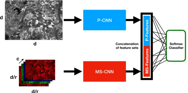
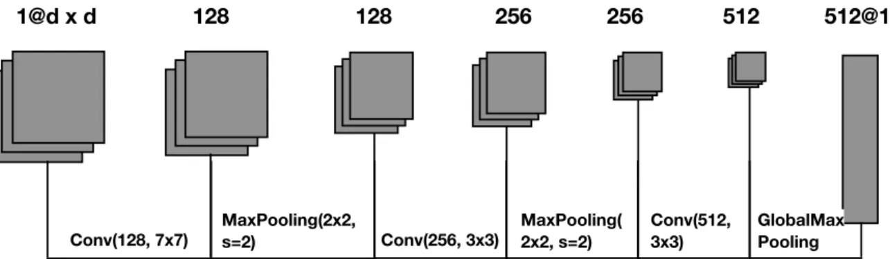
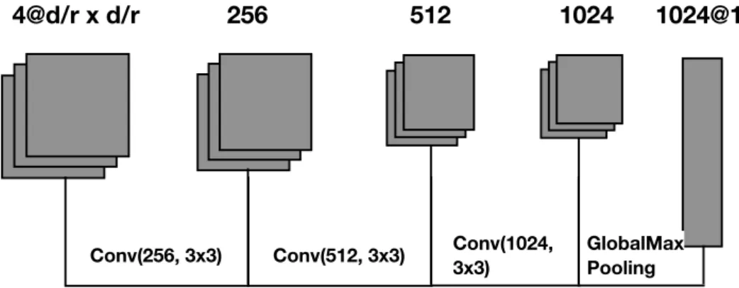
A Two-Branch CNN Architecture for Land Cover Classification of PAN and MS Imagery
Texte intégral
Figure


Documents relatifs
Lladó, “Multiple sclerosis lesion detection and segmentation using a convolutional neural network of 3d patches,” MSSEG Challenge Proceedings: Multiple Sclerosis
The CNN is trained to maxi- mize the Dice score (equation 3), which is a compromise between precision (equation 2 and sensibility 1 as detailed in equation 4 aimed at reducing
Recently, new approaches based on Deep Learning have demonstrated good capacities to tackle Natural Language Processing problems, such as text classification and information
Sidib´ e, Ex- ploration of Deep Learning-based Multimodal Fusion for Semantic Road Scene Segmentation, in: VISIGRAPP 2019 - Proceedings of the 14th International Joint Conference
While in some works a secondary model was used as a source of contextual information flowing into the object detector, our design will attempt to reverse this flow of
After an overview on most relevant methods for image classification, we focus on a recently proposed Multiple Instance Learning (MIL) approach, suitable for image
Performance (mAP in %) comparison in terms of different methods and visual features algorithms on Corel5k. We evaluate the returned keywords in a class-wise manner.
The global recall, mean recall and mean JI statis- tics have been traditionally employed to evaluate different image segmentation results, however, these metrics are not
