THE EFFECT OF A SHALLOW LOW VISCOSITY ZONE ON MANTLE CONVECTION AND ITS EXPRESSION
AT THE SURFACE OF THE EARTH by
Elizabeth M. Robinson B.S., Reed College, 1982
SUBMITTED IN PARTIAL FULFILLMENT OF THE REQUIREMENTS FOR THE DEGREE OF
DOCTOR OF PHILOSOPHY at the
MASSACHUSETTS INSTITUTE OF TECHNOLOGY and the
WOODS HOLE OCEANOGRAPHIC INSTITUTION
AUGUST 1987
Elizabeth M. Robinson, 1987
The author hereby grants to MIT and WHOI permission to reproduce and distribute copies of this thesis document in whole or in part.
Signature of Author
Joint Programin-Marine Geology and Geophysics, Massachusetts Institute of Technology and the Woods Hole
Oceanographic Institution Certified by
Accepted by
Barry Parson esis Supervisor
Chairman of the Joint Committee for Marine Geology and Geophysics, Massachusetts Institute of Technology and the
wiTmDRAWN
Woods Hole Oceanographic Institution2
THE EFFECT OF A SHALLOW LOW VISCOSITY ZONE ON MANTLE FLOW AND ITS EXPRESSION AT THE SURFACE OF THE EARTH
by
Elizabeth M. Robinson
submitted to the Massachusetts Institute of Technology/ Woods Hole Oceanographic Institution Joint Program in
Geology and Geophysics on July 1, 1987, in partial fulfillment of the requirements for the degree of
Doctor of Philosophy. ABSTRACT
Many features of the oceanic plates cannot be explained by conductive cooling with age. A number of these anomalies require additional convective thermal sources at depths
below the plate: mid-plate swells, the evolution of fracture zones, the mean depth and heat flow relationships with age and the observation of small scale (150-250 km) geoid and topography anomalies in the Central Pacific and Indian oceans. Convective models are presented of the formation and evolution of these features. In particular, the effect
of a shallow low viscosity layer in the uppermost mantle on mantle flow and its geoid, topography, gravity and heat flow expression is explored. A simple numerical model is
employed of convection in a fluid which has a low viscosity layer lying between a rigid bed and a constant viscosity region. Finite element calculations have been used to
determine the effects of (1) the viscosity contrast between the two fluid layers, (2) the thickness of the low viscosity zone, (3) the thickness of the conducting lid, and (4) the Rayleigh number of the fluid based on the viscosity of the lower layer.
A model simple for mid-plate swells is that they are the surface expression of a convection cell driven by a heat flux from below. The low viscosity zone causes the top
boundary layer of the convection cell to thin and, at high viscosity contrasts and Rayleigh numbers, it can cause the boundary layer to go unstable. The low viscosity zone also mitigates the transmission of normal stress to the
conducting lid so that the topography and geoid anomalies decrease. The geoid anomaly decreases faster than the topography anomaly, however, so that the depth of
compensation can appear to be well within the conducting lid. Because the boundary layer is thinned, the elastic plate thickness also decreases and, since the low viscosity allows the fluid to flow faster in the top layer, the uplift time decreases as well. We have compared the results of this modeling to data at the Hawaii, Bermuda, Cape Verde and Marquesas swells, and have found that it can reproduce their
observed anomalies. The viscosity contrasts that are required range from 0.2-0.01, which are in agreement with other estimates of shallow viscosity variation in the upper mantle. Also, the estimated viscosity contrast decreases as the age of the swell increases. This trend is consistent with theoretical estimates of the variation of such a low viscosity zone with age.
Fracture zones juxtapose segments of the oceanic plates of different ages and thermal structures. The flow induced by the horizontal temperature gradient at the fracture zone initially downwells immediately adjacent to the fracture zone on the older side, generating cells on either side of the plume. The time scale and characteristic wavelength of this flow depends initially on the viscosity near the
largest temperature gradient in the fluid which, in our model, is the viscosity of the low viscosity layer. They therefore depend on both the Rayleigh number and the
viscosity contrast between the layers. Eventually the flow extends throughout the box, and the time scales and the characteristic wavelengths of the flow depend on the
thickness and viscosity of both layers. When the Rayleigh number based on the viscosity of the top la er, and the depth of both fluid layers, is less than 10 , the geoid anomalies of these flows are dominated by the convective signal. When this Rayleigh number exceeds 106, the geoid anomalies retain a step across the fracture zone out to
large ages. We have compared our results to geoid anomalies over the Udintsev fracture zone, and have found that the predicted geoid anomalies, with high effective Rayleigh numbers, agree at longer wavelengths with the observed anomalies and can produce the observed geoid slope-age
behaviour. We have also compared the calculated topographic steps to those predicted by the average depth-age
relationships observed in the oceans. We have found that only with a low viscosity zone will the flow due to fracture zones not disturb the average depth versus age
relationships.
We have also applied the model to a numerical study of the effect of a low viscosity zone in the uppermost mantle
on the onset and surface expression of convective
instabilities in the cooling oceanic plates. We find that the onset and magnitude of the geoid, topography and heat flow anomalies produced by these instabilities are very
sensitive to the viscosity contrast and the Rayleigh number, and that the thickness of the low viscosity zone is
constrained by the wavelength of the observables. If the Rayleigh number of the low viscosity zone exceeds a critical value then the convection will be confined to the low
viscosity zone for a period which depends on the viscosity contrast and the Rayleigh number. The small scale
convection will eventually decay into longer wavelength convection which extends throughout the upper mantle, so
that the small scale convective signal will eventually be succeeded by a longer wavelength signal. We compare our model to the small scale geoid and topography anomalies
observed in the Southeast Pacific. The magnitude (0.50-0.80 m in geoid and 250 m in topography), early onset time (5-10 m.y.) and lifetime (over 40 m.y.) of these anomalies suggest
a large viscosity contrast of greater than two orders of magnitude. The trend to longer wavelengths also suggests a high Rayleigh number of near or over 10 and their original
150-250 km wavelength indicates a low viscosity zone of 75-125 km thickness. We have found that the presence of such small scale convection does not disturb the slope of the depth-age curve but elevates it by up to 250 m, and it is not until the onset of long wavelength convection that the depth-age curves radically depart from a cooling halfspace model. In the Pacific, the depth-age curve is slightly elevated in the region where small scale convection is observed and it does not depart from a halfspace cooling model until an age of 70 m.y.. Models that produce the small scale anomalies predict a departure time between 55 and 65 m.y.. These calculations also predict an asymptotic heat flow on old ocean floor which is higher than the plate model and between 50 and 55 mW/m2. This value agrees with measurements of heat flow on old seafloor in the Atlantic. In conclusion, we prefer an approximate model for the viscosity structure of the upper mantle which initially has a 125 km thick low viscosity zone that represents a
viscosity contrast of two orders of magnitude. The
viscosity contrast decreases as the plate ages to one order of magnitude or less by 130 m.y., and the low viscosity zone may also thicken with age. Finally, the Rayleigh number of the upper mantle is at least 105
and may be as large as 107.
With this model, the evolution of the surface plates would initially involve small scale convection which is driven by shear coupling to instabilities downstream and to small scale convection associated with fracture zones. This convective flow would begin at close to 5 m.y. and remain confined to the low viscosity zone until nearly 40 m.y.. As this convective flow cools the upper mantle beneath the low viscosity zone, longer wavelength convection begins
throughout the upper (or whole) mantle, and the heat
transport from the longer wavelength convection flattens the depth-age curve and may form swells.
Thesis Supervisor: Barry Parsons
5
ACKNOWLEDGMENTS
First, and foremost, I would like to thank my advisor, Barry Parsons, for his dedication to teaching me to be a
scientist. One day, before I started to work on this thesis, Barry said: "The only thing that I can teach you which you need to learn is PATIENCE." Well, rather
uncharacteristically, Barry was wrong in that I learned many things other than that from him. However, he was right that
I needed more patience. Unfortunately, after the three or four years that I have worked with Barry, I cannot say that I have fully acquired this desirable personality trait, but I can hope that the lessons that I have learned about
patience and the quality and completeness of good scientific research will stay with me and my work.
Besides my advisor many other people contributed to the completion of this work. Steve Daly taught me the ins and outs of the convection code and the art of convection
modelling. Mavis Driscoll familiarized me with the geoid anomalies and geoid-age relationships at fracture zones, and told me about many tips to make the thesis process easier. Marcia McNutt introduced me to the world of research and
academia, and has always afterwards provided me with fresh views on my research and those of others. Tom Jordan, Joe Pedlosky and Marc Parmentier thoroughly read and commented
on this thesis, and gave insights into the physical processes involved in these problems. Ros Binks, Linda Meinke and Dave Krowitz helped me tame the computers (the
monsters). Tina, Inna, Nina, Lyle, and Carol (Raimey) provided a buffer from the innumerable administrative
hassles at MIT and Oxford. And, Bill Brace funded me in the last few months of my graduate tenure. At the end of each chapter, specific acknowledgments are also given.
My friends at MIT and Oxford, who were there to talk, to watch basketball, to play bridge or just to hang out, are too many to name. I hope they know that I hold them very dear and each for their own characteristics. However, a special thanks goes to my office-mate for 3-4 years, Karen Fischer, for without her I might have lost my sanity. I would also like to thank everyone on the eighth floor at MIT and everyone in the computer room/graduate student offices at Oxford for providing an excellent place to develop and
finish this thesis.
My family also deserves a lot of credit. My mother did everything that she could from Seattle to make my life as easy and fun as possible in Boston. My brother and his wife provided an infinite amount of support, especially during my
first years in Boston while they lived in the suburbs up north. And, my sisters (Chris and Laura) and their spouses
(Randy and Mark), and Aunt Jean, Uncle Wes and my cousins were always there to talk and to visit. I couldn't ask for
a better family.
Finally, an especially important thanks goes to Alan Leinbach, for it is with him that I have shared the agony and exultation that marked the creation of this thesis. His
7
love and support helped me through the worst of the times and, thank God, he knows how to have fun too.
I dedicate this thesis to my parents. To my father, who died when I was 16, but had already given me the wisdom and love of a lifetime; and, to my mother, whose wisdom and love I cherish every day.
TABLE OF CONTENTS Abstract... Acknowledgments... Note... Chapter 1 - Introduction... 1.1 Overview... 1.2 Forward Modelling of Co 1.3 Numerical Modelling of Convection... 1.4 The Viscosity Structure 1.5 This Thesis...
Figure Captions ....
Figures... Chapter 2 - The Apparent Compe
2.1 Introduction... 2.2 Convection Calculations 2.3 Topography, Geoid & Gra 2.4 Results... 2.5 Conclusions... Acknowledgments... Tables... Figure Captions .... Figures...
Chapter 3 - The Formation of M
3.1 Introduction... 3.2 Numerical Model of the 3.3 Convective Flow... 3.4 Calculation of the Surf 3.4.1 Topography, Gr 3.4.2 Heat Flow... 3.4.3 Depth of Compe 3.4.4 Elastic Plate 3.4.5 Uplift Time... 3.5 The Theoretical Surface 3.6 Comparison to the Data. 3.6.1 Hawaii... 3.6.2 Bermuda... 3.6.3 Cape Verde.... 3.6.4 The Marquesas. 3.7 Discussion... 3.8 Conclusions... Acknowledgments... Tables... Figure Captions... nvective High Rayl Flow in the eigh Number of the Upper M nsation of Mid-vity Response F id-Plate Swells ow... .ce Expression. .. ity and Geoid
sation... rhickness... ... o... aExpexprssion... Mantl ... .. . 20 antle...22 Plate Swells unctions.... .25 .28 .29 .33 .33 .38 .43 ... 47 ... 52 ... 56 ... 57 ... 59 ... 62 ... 74 ... ... ... 74 ... ... 81 ... 85 ... ... 88 .. ... 89 ... ... 90 ... ... .. 90 ... ... 91 ... .... 92 ... 93 .. ... 97 ... 100 ... ... 100 ... 101 ... . .. 102 ... 103 ... 105 ... . .109 ... . . 110 .. ... 113 Figures... ... 118 Figures ...
Chapter 4 - The Mantle Flow & Geoid Anomalies at Fracture Zones... ... 4.1 Introduction... 4.2 Convective Flow... 4.3 Calculation of the Geoid & Topography Anoma 4.4 The Geoid Anomaly and the Geoid Slope with 4.5 Comparison to the Udintsev Fracture Zone... 4.6 Depth Versus Age... 4.7 Discussion... ... 4.8 Conclusions... Acknowledgments... Tables... ... Figure Captions... Figures... Chapter 5 - Instabilities in the Cooling Oceanic P
5.1 Introduction... 5.2 The Numerical Model... 5.3 Convection Induced by Cooling from Above... 5.4 Geoid, Topography, Gravity and Heat Flow... 5.5 Depth-Age, Geoid-Age and Heat Flow-Age... 5.6 Comparison to the Data... 5.7 Conclusions... Acknowledgments... Tables... Figure Captions... Figures... Chapter 6 - Conclusions... 6.1 The Convective Flow... 6.2 The Topographic, Geoid, Gravit
Response to the Convective Anomalies at Depth... 6.3 Constraints on the Viscosity S
Upper Mantle... 6.4 Some Final Conclusions... endix - The Numerical Method... A.1 Stokes Flow Formulation for Fi A.2 Penalty Function Formulation f A.3 Matrix Formulation of the Stok
Function . ..0... .. of Grid A.4 Resolution as References... List of Calculations y & Heat Flow Temperature ... 0... tructure of t nite Elements ... 134 lies. Age.. lates he .134 .140 .152 .155 .161 .163 .166 .170 .174 .176 .178 .184 .214 .214 .220 .226 .234 .239 .246 .253 .258 .259 .261 .267 .290 .290 ... 293 ... 295 ... 299 ... 301 ... 301 or the Pressure...301 es Flow Problem...304 Size .306 .309 .318 App
Note
Each chapter was written to stand alone as a
description of one or all of the problems considered in this thesis. The reader may then pick and choose the chapters
that he/she would like to read, and expect to fully understand the problem and its resolution. However, a certain amount of repetition must then occur between the chapters, and I hope that the more comprehensive reader will forgive the extra explanation.
Chapter 1: INTRODUCTION
1.1 Overview
The Earth's mantle deforms in response to a number of driving forces including earthquakes and glacial loads. However, the dominant form of deformation in the mantle is due to convective currents, driven by the residual heat from the formation of the Earth and the decay of radioactive
elements (Turcotte and Oxburgh, 1967; Knopoff, 1967;
McKenzie, 1969; Richter, 1973; McKenzie et al., 1974; Yuen et al., 1981). The discovery of viscous flow in the mantle grew out of the plate tectonic revolution in the earth
sciences during the mid-1960's. In particular, the plate tectonic description of the deformation of the surface of the Earth established that seafloor is continually destroyed
at subduction zones and replenished at mid-ocean ridges, and consequently that the mantle must flow to accommodate this transport of material (Turcotte and Oxburgh, 1967; Richter and McKenzie, 1978).
As developments in the plate tectonic hypothesis
continued, the driving force for the movement of the oceanic plates was presumed to be forces exerted on the plates by
convection in the mantle (Turcotte and Oxburgh, 1967;
Peltier, 1974; Yuen et al., 1981). Under this assumption, the plates are the visible expression of the top boundary of a convection cell and the convective flow represented by the plates is the dominant large scale flow pattern in the
mantle. However, the connection between the convective flow in the mantle and the motions of the plates at long
wavelengths remains unclear (Forsyth and Uyeda, 1975). In particular, the description of the oceanic plates as a conductively cooling thermal boundary layer has proved
inadequate in explaining a number of observed features of the plates (Parsons and Sclater, 1977; Detrick, 1981).
In this thesis, we explore models of the formation of the most prominent of these features: mid-plate swells
(Chapters 2, 3 and 5), the geoid anomalies and geoid-age relationships at fracture zones (Chapter 4), the flattening of the depth-age and the heat flow-age curves (Chapter 5), and the recent observations of short wavelength geoid
anomalies in the SEASAT data over the Central Pacific and Indian oceans (Chapter 5). The important similarity between these features is that they each require a thermal source or non-conductive cooling at depth. We briefly present them here in order of decreasing wavelength.
At young ages in the oceanic plates, conductive cooling mechanisms in the mantle can produce the observed depth-age
and heat flow-age relationships (Parsons and Sclater, 1977). In Figure 1.1, we have drawn the mean depth data as a
function of the square root of time in the North Pacific and North Atlantic (from Parsons and Sclater, 1977). For
comparison, we have also drawn the depth-age curve that is predicted by conductive cooling in the mantle. At ages
conductive cooling model, and the conductive cooling
mechanism appears to be retarded. Evidence also suggests that the heat flow-age curve flattens (Sclater and
Francheteau, 1970; Parsons and Sclater, 1977). Estimates of the initial time of flattening in the heat flow-age
relationship have until recently been close to 120 m.y. (Parsons and Sclater, 1977), but recent evidence suggests that it may flatten earlier (Detrick et al., 1986; Louden et al., 1987). To produce these deviations in the depth-age and heat flow-age curves, a thermal source is required to supply heat to the base of the plate, over and above that supplied by conductive mechanisms. Parsons and McKenzie
(1978) hypothesize that the flattening of the depth-age and heat flow-age relationships may be due to heat transport
from convective instabilities in the cooling oceanic plates. In fact, Parsons and McKenzie (1978) have showed that
oceanic plates can go convectively unstable in the region under the rigid portion of the plate in their lifetimes, and Houseman and McKenzie (1982) have also showed that these
instabilities would flatten the depth-age curve.
Mid-plate swells are regions of the seafloor associated with geoid, gravity, topography and heat flow highs in an
intermediate (1000-2000 km) wavelength range (Dietz and Menard, 1953; Crough, 1978; Detrick and Crough, 1978). In Figure 1.2, we show the geoid field over the Bermuda swell. The characteristics of swells are described in greater
underneath swells in comparison to the surrounding plate, however, a thermal source must exist below the surface. Such a thermal anomaly can also explain the geoid, gravity and topography anomalies (Dietz and Menard, 1953; Crough, 1978; Detrick and Crough, 1978; Von Herzen et al., 1982; McNutt and Shure, 1986). Many researchers believe that this thermal anomaly is created by an upwelling in the mantle and that mid-plate swells are the surface expression of
concentrated upwellings in a convective flow (Dietz and Menard, 1953; McKenzie et al., 1980).
Other observed but currently unexplained features are the geoid slope-age relationships that are inferred from the geoid anomalies at fracture zones. Fracture zones are
boundaries between plate segments of different age. In the conductive cooling models of the plates, since each plate segment has undergone a different amount of cooling, the depth and geoid heights differ across the fracture zone and, in both depth and geoid, the anomalies contain a step at the
fracture zone. Recent data which constrains the geoid-age relationship at fracture zones shows that steps are evident
in the geoid anomalies (see Figure 4.17) but that they do not evolve, as the plate segments cool, in accordance with either the halfspace or thermal plate models (see Figure
4.18). Furthermore, the observed geoid slope-age
relationships vary from fracture zone to fracture zone (Cazenave et al., 1984). For example, entirely different geoid slope-age relationships are found at the Mendocino,
Eltanin, Udintsev and Falkland-Agulhas fracture zones (Sandwell and Schubert, 1981; Detrick, 1982; Cazenave et al., 1984; Driscoll and Parsons, 1987; Freedman and Parsons,
1987). The geoid slope-age relationship measures long wavelength changes in the geoid field at fracture zones. Therefore, the deviations from the conductive cooling models that are observed in the geoid slope-age relationships at
fracture zones and the variability between fracture zones must be due to sources that are not confined to an area near
each fracture zone, but that affect the broad regions around them. Since the temperature gradient between lithosphere of differing age across the fracture zone will drive convection in a viscous Earth, the variability in the geoid anomalies and the geoid-age relationships at fracture zones may also be explained by the convective flow underneath them (Craig and McKenzie, 1986).
The final unexplained feature of the oceanic plates was discovered in the SEASAT data set. The SEASAT satellite samples the surface height of the oceans which closely approximates the Earth's geoid (Talwani, 1970). This data set has an accuracy of better than 10 cm and a ocean-wide coverage with a resolution of near 100 km between tracks
(Tapley et al., 1982). In the Central Pacific at ages of 5-40 m.y. and in the Central Indian Ocean, 150-250 km
wavelength geoid anomalies with amplitudes of 0.50-0.80 m have been observed, with a possible trend towards longer wavelengths with age (Haxby and Weissel, 1986; Cazenave et
al., 1987). The anomalies are lineated parallel to the motion of the Pacific plate (Haxby and Weissel, 1986). A shipboard study along several SEASAT tracks over young ocean floor in the Central Pacific found that the geoid anomaly was also associated with a topographic anomaly of close to 250 m (pers. comm. Parsons, 1987). The shiptracks and two sets of the gravity and topography lines from this oceanic cruise are drawn in Figure 1.3. In line 1 (Figure 1.3(a)),
just west of the East Pacific Rise, no signal is present. By line 2, however, which is parallel to the East Pacific Rise on 6 m.y. old crust, a 150-250 km wavelength signal is
apparent. The signal in the gravity line correlates with the signal in the topography line, and its magnitude, 10-15 mgals, confirms the geoid estimates of the anomaly. Since the geoid and topography anomalies correlate between tracks
in a direction that is oblique to the fracture zone trend but parallel to plate motion, they most likely must also be
due to a source beneath the plates (Haxby and Weissel, 1986). Buck and Parmentier (1986) and Haxby and Weissel
(1986) propose that these anomalies are the surface
expression of instabilities in the cooling oceanic plates which were originally hypothesized to produce the flattening
of the depth-age and heat flow-age curves. However, an immediate problem is apparent with this explanation, since the small scale anomalies are evident at 5-40 m.y. in age
and the flattening of the depth-age curve does not occur
---until 70 m.y.. Nevertheless, this explanation seems likely given the nature of the lineated anomalies.
In summary, each of these features requires a thermal source at depths beneath the rigid portion of the plates. Two processes produce thermal anomalies in the mantle: enhanced radioactivity and thermal convection (Roberts,
1967; Runcorn, 1969; McKenzie et al., 1974; Jarvis and Peltier, 1982). However, in an explanation of each of the above features, a convective source seems most likely.
Since very different convective flows can produce the same geoid, gravity, topography and heat flow anomalies at the surface, the inversion of the data for the thermal
source function is nonunique (Parker, 1977). Since the inverse problem is not well posed (at least at present), however, we can only forward model each of the problems,
i.e. take a parameterized model of the mantle and vary its parameters until a good fit to the data is achieved. With this approach, there is no guarantee that the set of
parameters which give the best fit to the data is unique and that the correct solution has been isolated (Backus and
Gilbert, 1967; Backus and Gilbert, 1968). However, given the correct rheological structure for the mantle and the boundary conditions on the flow and the temperature that bound it, the convective flow is then determined. The
inverse problem is then reduced to the determination of the nature of the rheological structure and the boundaries on flow in the mantle. Therefore, the emphasis must be placed
on gaining an understanding of the essential physics which governs the variation of these parameters and, as more
constraints are placed on the flow and on the rheological properties of the mantle by the data, a better model can be
achieved.
1.2 Forward Modelling of Convective Flow The first mathematical descriptions of thermal
convection were developed in the late 19th century. Two of the most significant theoretical developments towards the understanding of convective flow were made by Lord Rayleigh and Osborne Reynolds. They found that, given a set of
boundary conditions, any convective flow can be
characterized by two nondimensional numbers which are now called the Rayleigh number (Rayleigh, 1916) and the Reynolds number. In practice, the Rayleigh number-is proportional to the ratio between the time that it takes to heat a layer of fluid by conduction and the time that it takes a particle of fluid to circulate once around the convective cell. The Reynolds number represents the ratio of the inertial forces to the viscous forces. Since the Reynolds number in the Earth is very small (around 10-10), the inertial forces are negligible when compared with the viscous forces (Turcotte and Oxburgh, 1967; McKenzie, 1969; McKenzie et al., 1974).
In the mantle, the Rayleigh number is the most
significant parameter that governs the flow (Turcotte and Oxburgh, 1967; McKenzie, 1969; McKenzie et al., 1974).
19
Without the effects of internal heat generation included, the Rayleigh number, Ra, can be given by:
Ra = gcxATd 3/gK (11)
where g is the acceleration of gravity, a is the thermal expansion coefficient, AT is the temperature difference
across the fluid layer, d is the depth of the fluid layer, p is dynamic viscosity and K is thermal diffusivity.
Estimates of the magnitude of the Raleigh number in the upper mantle in the literature range from 106 to 107, where the variation in the estimate is due to the uncertainty in the magnitude of the physical parameters, g, a, AT, d, p
and K, (McKenzie, 1967; Richter, 1973; McKenzie et al., 1974). Since the Rayleigh number can scale laboratory
results to apply to mantle flow, experiments have been done that empirically, as well as theoretically, reveal the
nature of Rayleigh-Bernard convective flow in a viscous fluid as its Rayleigh number increases to mantle values in three-dimensions (Busse, 1967; Busse and Whitehead, 1971). Below a critical Rayleigh number, the fluid will not
convect, but transport heat by conduction. Above this critical number, which is near 103 and depends upon the boundary conditions, the fluid convects in two dimensional cylindrical cells and arranges its "plan form" (the spatial orientation of the convective flow pattern) in response to the initial temperature disturbance. When the Rayleigh number is increased to values above 2x10⁴, from an initial two dimensional cylindrical flow pattern, two dimensional
cells are no longer stable and the flow becomes three
dimensional. Another set of cells grows up perpendicular to them, forming an overall pattern which is called "bimodal" convection. Above a Rayleigh number of 105, the bimodal convection pattern in turn becomes unstable and the flow assumes a "spoke" pattern. The spoke pattern is
characterized by thin, intense sites of upwelling and broad, diffuse downwellings. Above this range of Rayleigh numbers, laboratory experiments with a negligible Reynolds number are very difficult (Busse and Whitehead, 1971; Busse and
Whitehead, 1974; Richter and Parsons, 1975; McKenzie, 1983). Therefore, most of our knowledge of flow at these Rayleigh numbers comes from numerical models of the flow.
1.3 Numerical Modelling of High Rayleigh Number Convection In 1974, McKenzie et al. published the first numerical model of flow in the mantle at Rayleigh numbers up to 106.
Using finite difference numerical techniques and assuming that the flow was two-dimensional and that the viscosity of the fluid was constant, they confirmed the theoretical
prediction that the advection of heat would occur primarily in small boundary layers at the edges of the cell and that the interior of the cell was nearly isothermal. As the Rayleigh number increased, the vigor of the convection increased and the boundary layers thinned.
Many researchers have since explored more realistic rheological models of the mantle than a uniform constant
21
viscosity upper mantle. In particular, studies with a temperature and pressure dependent viscosity structure and other nonlinear rheologies have provided insights into the effects of the rheology on convective flow at high Pradtl numbers (Parmentier, 1978; Yuen et al., 1981; Yuen and Fleitout, 1984; Fleitout and Yuen, 1984a; Buck and Parmentier, 1986). However, these studies are time
consuming on computers and are therefore expensive, so that only a limited number of rheologies have been tested. Since we do not know the exact rheology of the mantle, the results
are very difficult to apply to mantle flow.
We approach the problem differently. Instead of
attempting to understand the fluid flow in the presence of a complex rheology, we try instead in one suite of
calculations to fully explore the effect of only one feature which is expected from estimates of the rheology of the
mantle and from observational data. Then the physical effect of that component of the model can be built upon as more complex models are studied. In this thesis, we have built upon studies of the effect of a conducting lid at the
surface of the mantle, representing an oceanic plate, and have added a low viscosity zone in the uppermost mantle.
Such a layer is indicated not only by theoretical results but observational results as well.
As a note, because the computer time that would be required to fully explore the flow in three dimensions is prohibitively large, these results and the results that we
present in this thesis are limited to two dimensions.
However, we know that at large Rayleigh numbers, the flow is three-dimensional as in the "spoke" pattern. With a two-dimensional model, flow in and out of the plane of the
calculation, the effects of three-dimensional perturbations to the flow and three-dimensional instabilities are not included. These effects may strongly affect the results and, in each of the problems that we consider, we will discuss the specific effects that we have ignored by only addressing two-dimensional flow.
1.4 The Viscosity Structure of the Upper Mantle
Due to the large temperature gradient from the surface to the interior of the mantle, the largest viscosity change in the mantle is at the surface of the Earth and results in the strength of the surface plates. The presence of plates, which act dynamically like conducting lids at the surface,
affects the convective flow in three ways. First, since the thermal structure of the top portion of the plates is cool
enough so that the plate is rigid, the mantle can flow beneath it, separate from the conducting lid. Second, the
convective temperature anomalies are depressed to greater depths than in a constant viscosity model. Third, the plates absorb a portion of the temperature difference
between the interior of the convection cell and the surface through conduction, so that the magnitude of the temperature anomalies decreases as the thickness of the conducting lid
23
increases (Houseman and McKenzie, 1982; Jaupart and Parsons, 1985; Buck and Parmentier, 1986). Due to the last two
effects, the geoid, gravity, topography and heat flow anomalies decrease as the plate thickness increases in thickness (Buck and Parmentier, 1986).
The viscosity structure of the mantle beneath the plates is not well known. What little evidence of the viscosity structure in the upper and lower mantles comes
from laboratory results, inferences from seismic velocity anomalies, modelling of post-glacial rebound, and
theoretical calculation of the viscosity structure based on estimates of the temperature and pressure structures in the mantle. According to each of the indicators (that would be sensitive to viscosity changes in 100-200 km layers),
however, the most prominent feature in the uppermost mantle is a low viscosity zone underneath the oceanic plates
(Anderson and Sammis, 1970; Solomon, 1972; Peltier, 1974; Weilandt and Knopoff, 1982; Bott, 1985). Cooper and
Kohlstedt (1984) have shown with laboratory experiments on olivine that melt in the intersections between grains will cause the diffusion path length through an aggregate of these grains to decrease. Therefore, the presence of melt
in the uppermost mantle would decrease its viscosity and change its deformation behavior. From calculations of
partial melting in the mantle, melt production is thought to be confined to the top 200 km of the upper mantle (e.g.
a shallow layer with a small degree of melt throughout the oceanic mantle underneath the plates (Anderson and Sammis,
1970; Solomon, 1972). In particular, the most prominent seismic feature in the uppermost mantle is a low velocity zone extending from near 60 km to 150 km (Weilandt and Knopoff, 1982; Bott, 1985). Since this region is also associated with high attenuation, the most widely accepted explanation of its origin is that it contains a small
fraction of melt (Anderson and Sammis, 1970). Therefore, the presence of the melt in the top 200 km of the mantle would create a low viscosity zone which extends from the base of the rigid portion of the plates to 200 km. Finally,
the experimentally determined exponential relationship
between viscosity and temperature and pressure also predicts a low viscosity zone underneath the plates (Parmentier, 1978; Fleitout and Yuen, 1984; Buck and Parmentier, 1986). In the thermal boundary layer at the surface, the viscosity will rapidly decrease due to the large temperature gradient with depth. Then, in the adiabatic mantle the viscosity will increase due to the increase in pressure with depth. Beneath the plates and before the pressure causes the viscosity to increase to larger values, the viscosity is low, effectively creating a low viscosity zone underneath the plates (of at least one or two orders of magnitude less than the ambient mantle viscosity).
Theoretical calculations of the viscosity structure with temperature and pressure also predict that the low
viscosity zone will decrease in magnitude and thicken with age (Buck and Parmentier, 1986). However, theoretical constraints on melting in the mantle indicate that melting will always be confined by the effects of pressure to a depth above 200 km in the uppermost mantle (e.g. McKenzie, 1981). Therefore, when both the temperature and pressure and the melting effects are included in the calculation of a theoretical viscosity structure, the low viscosity zone may remain close to its original thickness (above 200 km in depth and below the conducting lid) and viscosity contrast for longer than predicted when only the effects of
temperature and pressure included. In fact, seismic
evidence indicates that a low velocity zone (and, therefore, a region of partial melt) is measurable in the uppermost mantle, above 200-400 km, throughout much of the oceanic mantle (Weilandt and Knopoff, 1982).
1.5 This Thesis
In this thesis, we have explored the effect of a low viscosity zone on mantle flow and its geoid, gravity, topography and heat flow expression at the surface of the Earth. In particular, we have modelled the anomalous
features that were described in section 1.1. We use a finite element numerical method to model the flow with a simple three layer viscosity structure for the upper mantle
(Hughes et al., 1979; Daly and Raefsky, 1985). The
The viscosity model consists of a conducting lid overlying a low viscosity zone which in turn overlies a constant
viscosity layer. The simplicity of the model allows us to explore a number of models where we vary the layer
thicknesses, the viscosity contrast (the ratio of the viscosity contrast in the top layer, pt, to that in the bottom layer: pt /b) and the Rayleigh number of the fluid.
To calculate the gravity, geoid, topography and heat flow anomalies at the surface that result from the flow, we use a Green's function method (Parsons and Daly, 1983).
We have found that with the addition of the low
viscosity zone the convective model not only qualitatively fits the observed anomalous features in the oceanic plates but quantitatively fits them as well. The convective models of mid-plate swells (Chapter 2 and 3), of fracture zones
(Chapter 4) and of the stability of the cooling oceanic plates (Chapter 5) are all very sensitive to a shallow low viscosity zone. With our model, by specifying only the thermal boundary conditions and the three layered viscosity structure, we are able to produce a complete model for the formation of mid-plate swells, in which both the surface anomalies and the origin of the thermal source was
explained. The same model (with the same range in the parameters which describe the viscosity structure) also predicts the geoid slope-age and depth-age behavior at fracture zones, the origin of the small scale anomalies in the Central Pacific and Indian oceans, and the flattening of
27
the depth-age and heat flow-age curves. Therefore, we are able to place significant constraints on the viscosity
contrast and the thickness of the low viscosity zone, which are consistent with theoretical estimates of the mantle viscosities. In particular, the viscosity contrast was
constrained to be greater than 0.1; the thickness of the low viscosity zone was determined to be 75-125 km. With the addition of a low viscosity zone, therefore, a convective model can produce many of the observed anomalous features in the oceanic plates.
Figure Captions
Figure 1.1: The depth-age data for the North Pacific and the North Atlantic oceans (solid line) plotted versus the square root of time. Figure taken from Parsons and Sclater
(1977). The predictions of the conductive cooling model are also drawn (dashed line).
Figure 1.2: Geoid anomalies in the region of the western North Atlantic which encompasses the Bermuda swell. The anomalies are derived from the SEASAT altimeter data set by removing a GEM 9 reference field up to degree and order 10 and by smoothing the resulting geoid anomalies onto a
uniform 50 km grid. Contour interval 1 m. Figure taken from Detrick et al. (1986).
Figure 1.3: (a) The shiptracks in the Central Pacific. (b) The gravity and topography data collected from lines 1 and 2, in Figure 2(a). The scales are alongside the lines. In
line 1, which is just west of the East Pacific Rise, there is no small wavelength signal. However, by line 2, which is on 6-10 m.y. old crust, the small wavelength signal is
2 000
NORTH PACIFIC
b Mew depM an staneW deviafen 3000 ..--- orecol elevation, plate model
--- Linw relation 4000 5000 0 ' 9 6000 -5 6 8 3 21 26 32 M4 MIS 25 7000 0 I 2 3 4 5 6 7 a 9 i1 10 1 .AGE (M Y 8 P) (a) ,AGE iM YIP) Mh
Figure 1.1
80*W 70* 600 50
S LINE I 4I to I2500 A V4 .3000
~~
i-'
i
,
4
AAi
iA'4XJ
500 200 i00 0 00 200 30o KM LINE 2 30 -A
10
x
-a
- -'.s., -- 3500 - - *00 S4 J40 Sb 300 300 300 0 100 300 500 KM Figure 1.3al .
r.A -- I
160 Fon
33
CHAPTER 2: THE APPARENT COMPENSATION OF MID-PLATE SWELLS
2.1 Introduction
Hot spot volcanic chains usually crest large regions of anomalously shallow seafloor, where the generally linear relationship between the long wavelength geoid and
topography anomalies supports a Pratt compensation model for the uplift. Analyses of the geoid and topography anomalies at most swells, however, give a depth of compensation for the swell topography which appears shallower than the
thermal plate thickness (Haxby and Turcotte, 1978; Crough, 1978). Estimates at various hotspot chains indicate depths of compensation of 60-90 km for the Hawaiian swell (Crough,
1978; McNutt and Shure, 1986), 40-70 km for the Bermuda Rise (Haxby and Turcotte, 1978), and 40-60 km for the Marquesas swell (Crough and Jarrard, 1981; Fischer et al., 1986). Because thermal cooling is thought to extend to near 125 km in depth underneath the seafloor surrounding these swells
(Parsons and Sclater, 1977), and because, when cooled,
mantle materials no longer deform so readily, these shallow compensation depths seem to pose a problem for the
explanation of hotspot swells as a natural consequence of mantle and plate dynamics.
The anomalous heat flow associated with mid-plate swells argues for a thermal origin for their uplift (Von Herzen at al., 1982; Detrick et al., 1986). Detrick and Crough (1978) pointed out that, by elevating the
34
temperatures underneath the Hawaiian swell, one could
explain its shallow depths and subsidence. If one assumes that the plate behaves rigidly down to depths near the
thermal plate thickness, as calculated from thermal cooling models (e.g. Parsons and Sclater, 1977), the elevation of the temperature structure must be accompanied by thinning of the rigid plate to a certain depth. By simply prescribing this depth, beneath which the plate is replaced by material at the ambient mantle temperature, one can fit the gravity and topography anomalies and the subsequent subsidence seen at Hawaii (Detrick and Crough, 1978; McNutt, 1984). The shallow depth of compensation is then a reflection of this thinner plate. The plate thinning that is required to
produce the observed anomalies is very large, as in the case of Hawaii, where the plate must be thinned from over 100 km in depth to just 40 km. However, the uplift time seen at Hawaii is very short, between 5 and 8 m.y. and, to produce the observed geoid and topography anomalies through
conduction within this uplift time, the heat flux that is required is excessively large (Detrick and Crough, 1978;
Emerman and Turcotte, 1983).
These short uplift times suggest an advective
mechanism. Other models of swells describe the uplift as the surface expression of a convection cell (McKenzie et al., 1980; Detrick et al., 1986). These models in principle provide a mechanism to instigate and maintain the swell and
35
explain the frequency and separation between swells as a consequence of the convection planform in the upper mantle but, if the thermal plate behaves rigidly down to depths
corresponding to the full thermal plate thickness, they cannot produce the shallow depths of compensation.
However, the viscosity of mantle material is
temperature and pressure dependent, so that the plate does not act rigidly to depths corresponding to the thermal plate thickness. To a rough approximation, one can divide the plate into two parts, the boundary between which is governed by the temperature (Parsons and McKenzie, 1978). In the upper portion, the conducting lid, the temperatures are sufficiently low that the material behaves rigidly. In the
lower portion of the plate where the temperatures are
higher, the material can deform ductily and can participate in the mantle flow. An upwelling plume can penetrate this layer and replace it with the hotter material. The
conducting lid behaves rigidly but, on a conductive time scale, thins due to heating from the plume.
Theoretical considerations and observational evidence suggest that the viscosity at depths around the thermal plate thickness can be quite small and that these low
viscosities extend to depths in the mantle below the thermal plate thickness. First, theoretical calculations of the viscosity with depth, which assume an exponential
temperature and pressure dependence and a temperature
show that the viscosity will decrease sharply to the base of the top thermal boundary layer in the mantle. In the
adiabatic region immediately below it, the pressure gradient with depth will cause the viscosity to slowly rise again forming a low viscosity zone (Buck and Parmentier, 1986). Second, since the presence of melt at grain boundary triple
junctions may shorten the diffusive path length through a conglomerate of grains thereby enhancing the creep rate, the segregation of melt in the upper mantle may produce a layer with an effectively lower viscosity (Cooper and Kohlstedt, 1984; McKenzie, 1985). Seismic studies of the asthenosphere and upper mantle show a marked increase in attenuation and a decrease in velocity beneath the lithosphere which is often interpreted as the seismic expression of a layer with a large proportion of melt (Anderson and Sammis, 1970;
Solomon, 1972). If this region is partially molten then, as predicted by the laboratory experiments of Cooper and
Kohlstedt (1984), there should be changes not only in its elastic behavior but in its deformational behavior as well. Third, Craig and McKenzie (1986) have studied convection at fracture zones, which is induced by the horizontal
temperature gradient at the base of the oceanic lithosphere. Their model is two-dimensional, and consists of a fluid
layer overlain by a conducting lid. They find that a thin, 150 km thick, low viscosity zone with an upper bound on the viscosity of 1.5x101 9 Pa.s (approximately two orders of magnitude less than the average viscosity of the upper
mantle as determined from studies of post-glacial rebound) under a conducting lid of 75 km can produce the general
character of the geoid and topography signatures at fracture zones.
Since in any convective model for mid-plate swells, the flow reflected by the swell and the large scale circulation containing the plates are decoupled, one might argue that a low viscosity zone is inherent in convective models of mid-plate swells. Without decoupling, localized upwellings would be sheared by the surface flow due to the plates. This decoupling requires a region of the mantle such as a low viscosity zone whose physical properties mitigate the transmission of shear stress between the two flow regimes. Because viscosity variations in the mantle can strongly alter the topographic and gravitational response to the dynamic processes beneath the plate, convection models must include such a zone to accurately represent the formation of the swell.
To study the effect of a low viscosity zone on the
convective formation of mid-plate swells, we have simplified the viscosity structure to a three layer model consisting of a conducting lid overlying a low viscosity zone which in turn overlies a constant viscosity layer extending to the base of the upper mantle (Figure 2.1). In this paper we discuss the effect of varying the thickness of the low viscosity zone, the viscosity contrast and the overall Rayleigh number (based on the bottom viscosity) on the
gravity, topography and geoid signatures of the flow and on the inferred depth of compensation for the swell topography. In particular, for given conducting lid and low viscosity zone thicknesses, we will show that by lowering the
viscosity in the layer we can produce arbitrarily small apparent depths of compensation.
2.2 Convection Calculations
The numerical model consists of a low viscosity layer sandwiched between a conducting lid and a constant viscosity layer, with uniform heating from below through a stress-free
boundary and with a constant temperature condition on the top boundary (see Figure 2.1). We have replaced the
dimensional variables (denoted with primes) with their nondimensional counterparts through the following
transformations: ' = 1o g (2.la) (x',z') = d(x,z) (2.1b) T' = AT T (2.lc) t' = (d2 /K) t (2.1d) P' = PO P (2.le)
where po is the reference kinematic viscosity, x and z are the horizontal and vertical coordinates respectively, t is
the time, d is the depth of the convecting layer, K is the thermal diffusivity, po is the reference density and AT is the reference temperature contrast given by the constant heat flux condition:
39
AT = Fd/Kp0Cp (2.lf)
where F is the prescribed flux and Cp the specific heat. To scale the results, we used the values for the physical
parameters given in Table 2.1.
Omitting the primes, the equation of motion, the heat transport equation and the equation of state are given by,
= -R(T-To)z (2.2)
BT/Dt + u.VT = V2T (2.3)
1 - adT(T - TO) = p (2.4)
where u is the velocity vector, a is the thermal expansion coefficient, z is a vertical unit vector, To is the
reference temperature, Y is the stress tensor given by:
Gij = - 8ij + p (Qbui/txj + BUjf/~Xi) (2.5) with p the pressure and R the Rayleigh number:
R = gocXATd3/goK (2.6)
where go is the acceleration of gravity. These equations are solved using a velocity based finite element method
(Daly and Raefsky, 1985). Although the incompressibility equation:
V.u = 0 (2.7)
is never solved explicitly, a penalty function treatment of the pressure forces incompressibility (Hughes et al., 1979). The boundary conditions on the flow are summarized in Figure 2.1.
All of the convection calculations were run to steady state with the implicit time stepping method described in Brooks (1981). To resolve the boundary layer flow, we often
used a nonuniform grid with double or quadruple the number of grid points in the vertical direction in the low
viscosity zone. We checked the resolution and steadiness of the flow by comparing the average flux through the elements at different depths to their steady state equilibrium
values. Also, due to the complex interaction of the up and downwelling plumes with the low viscosity zone, we ran the most extreme models on a uniform grid with an explicit
finite difference time stepping routine for a convective overturn time to check for convergence.
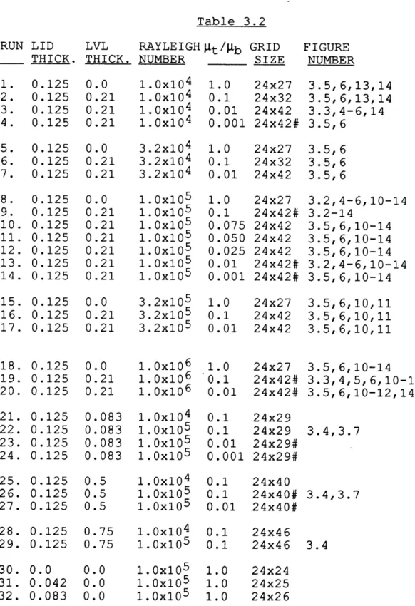
In Table 2.2, we present the parameters for three
suites of calculations chosen to illustrate the effect of a low viscosity zone on the convection and on the
corresponding surface observables. In all of these
calculations, the shear stress and vertical velocity are zero on the bottom boundary, and both components of velocity are zero at the base of the conducting lid, which is 0.125
(75 km) thick. In runs 1(a-c) in Table 2.2, we varied the viscosity in the low viscosity layer with a 0.21 (125 km) thick low viscosity zone and a Rayleigh number equal to 105.
In Figure 2.2, results for viscosity contrasts of 100, 101 and 102 are presented, and the variation of the horizontally averaged temperature and the longest wavelength component of the temperature structure with depth are given in Figure 2.3. Two essential points are illustrated by these
calculations. First, since the low viscosity zone causes the local Rayleigh number of the fluid encompassing the top
boundary layer to increase, the boundary layer thins.
Second, the low viscosity zone reduces the stresses near the base of the rigid lid facilitating horizontal fluid flow. We compared these runs to ones with no conducting lid and a
free top boundary. We found that this stress reduction and increased horizontal flow near the boundary caused the top boundary to look more like a free boundary to the rest of the flow and the boundary layer was correspondingly thinner.
In general, an order of magnitude decrease in viscosity in the low viscosity zone will thin the boundary layer to a thickness corresponding to an order of magnitude or more increase in the local Rayleigh number. At high viscosity contrasts, the upper boundary layer can surpass its local critical Rayleigh number and become unstable, generating instabilities which sweep into the downgoing plume. The instabilities grow with a period much less than the overturn time but have a negligible effect on the longest wavelength geoid, gravity and topography signals. Due to our limited computational ability at present, however, we cannot check the resolution of this instability and do not present cases in which the Rayleigh number based on the top viscosity exceeds 107
-In runs 2(a-c) in Table 2.2, we varied the Rayleigh number in the convecting layer from 104 to 106, with a 0.21
(125 km) thick low viscosity zone at a viscosity contrast of 0.1 and a 0.125 (75 km) thick conducting lid (Figure 2.4). Figure 2.5 shows the mean and first harmonics of the
temperature structures. As in Rayleigh-Bernard convection in a constant viscosity layer, the boundary layer thickness and mean temperature decrease with increasing Rayleigh
number (if AT is held constant).
In the final series of calculations (Figure 2.6), we varied the thickness of the low viscosity layer (parameter
'a' in Figure 2.1). In particular we compared two runs at a Rayleigh number of 105 where the top layer has either a
thickness of 0.08 (50 km) or of 0.5 (300 km) to the
calculation already discussed where the top layer is 0.21 (125 km) thick. Figure 2.7 contains the mean and first
harmonic temperature profiles for these runs. Initially, as the thickness of the low viscosity layer increases, the mean temperature decreases; and, at the intermediate layer
thickness of 0.21 (125 km), the magnitude of the mean
temperature profile is at a minimum for these runs. As the layer thickness increases further, however, the mean
temperature profile returns to the profile for the very thin low viscosity layer. This nonlinear behavior in the mean temperature profile reflects the trade off between the increase in the local Rayleigh number and the effective change in the top boundary condition which can appear
stress-free rather than rigid. When the low viscosity layer is thin, the boundary layer is not thinned by the change in the effective Rayleigh number of the top layer, but by the change in the apparent boundary condition. At the
by both the change in the effective Rayleigh number and the change in the apparent boundary condition to the minimum thickness observed. At a layer thickness of half of the fluid layer depth, however, the.boundary condition agains appears to be rigid, so that even though the layer is thinned by the change in the effective Rayleigh number of the top layer, the boundary layer is not as thin as in the case of the intermediate layer thickness.
For a layer 0.21 (125 km) or 0.5 (300 km), the
viscosity layering also modifies the side boundary layers. It makes the downwelling plume, which originated in the low viscosity zone, much thinner than expected for the given Rayleigh number and it pinches the upwelling plume as it enters the top layer. At the intermediate layer thickness, the viscosity transition occurs very near the regions of high vorticity of the convection cell and the spread of pinch-off of the flow that occurs as the plumes hit the
viscosity contrast augments the vorticity. This increase in vorticity may help to instigate the instabilities seen at high local Rayleigh numbers.
2.3 The Topography, Geoid and Gravity Response Functions To calculate the gravity, geoid and topography
anomalies for these calculations, we use the Green's function method formulated by Parsons and Daly (1983) in which the temperature field is decomposed into its Fourier components and, at each wavenumber, k, the Green's function
response of the gravity and topography to the temperature field, the gravity and topography kernels respectively, are calculated. The surface topography kernel represents the effect of a density anomaly at a depth, z, on the surface topography through the transmission of normal stress. It is always positive, and varies from one at the surface to zero at the bottom boundary. On the top boundary, the topography fully reflects a pressure perturbation at the surface so that the kernel equals one. On the bottom boundary, since the normal velocity is zero, the pressure perturbation is fully compensated by the topography on the bottom boundary and the kernel is zero. The gravity kernel, on the other hand, represents the sum of the gravitational effects of the topography on the boundaries and the density variations in the layer. Since a temperature source at a boundary
produces topography with unit weighting and since the topography and temperature variations are both at the
boundary, their gravitational effects cancel and the gravity kernel is always zero at the boundaries. Because the
gravity kernel reflects a trade off between the effect of boundary topography and temperature variations within the
layer it can change sign in the fluid layer.
The dimensional topography in the Fourier domain, h(k) is given by:
h' (k)=[po/ (po-pw) ]QATd h (k)
where H(k,z) is the topography kernel and where the prime denotes the nondimensional variable. The dimensional gravity, g(k), can also be written:
g' (k')=21cGpoaATd g(k)=27EGpomxATd G(k,z)T(k,z) dz (2.9a) where G(k,z) is the gravity kernel and G is the Universal Gravitational Constant. The gravity kernel can be expressed as the sum of contributions from the surface topography, the internal density differences and the bottom boundary
topography attenuated by the depth of the layer:
G(k,z) = H(k,z) -exp(-Iklz) + exp(-Ik|)Hb(k,z) (2.9b) where Hb(k,z) is the kernel for the bottom boundary
topography. Low viscosities in the top layer reduce the stress transmitted across the layer from buoyancy forces beneath it, so that the low viscosity zone primarily effects the first term in equation (2.9b). The low viscosity zone also alters the temperature structure in equation (2.9a), but this effect is minimal when compared to its effect on
the gravity kernels. Finally, the geoid anomaly is derived from the gravity anomaly using Brun's formula:
N'(k ) = g'(k)/Ik'1go = [2nGpoaATd2/g0 ] g(k)/k (2.10) where N is the dimensional geoid. For a two layer viscosity model, the kernels can be calculated analytically (Daly et al., 1984). For a general variable viscosity structure, however, we must numerically calculate them using a
predictor-corrector algorithm.
In Figure 2.8, we have drawn the gravity and topography kernels corresponding to runs 1(a-c) with a 0.125 (75 km)
conducting lid and a 0.21 (125 km) low viscosity zone. In the lid we have set the viscosity to 103, which effectively mimics rigid behavior. The low viscosity varies from 1.0 to 0.01. As the viscosity contrast increases, the low
viscosity zone damps the surface topography kernels at depth and their power is concentrated in the top portions of the model. The surface observables are dominated by the k=71 wavenumber, and can be well approximated by the effect of this harmonic alone. To calculate the observables, we have
obtained the kernels for each of the runs out to wavenumber k=8. For the shorter wavelengths (less than X=0.25), we have approximated the kernels by those for a two layer
structure of a rigid lid overlying a constant viscosity zone. Since the surface topography kernels are effectively zero before the base of the low viscosity zone, they are not affected by the viscosity jump. At the wavelength, X=2, the topography kernels are effectively zero at the base of the low viscosity zone for a viscosity contrast of two orders of magnitude. By this viscosity contrast, therefore, the
topographic response to the underlying convection is limited to depths corresponding to the conducting lid and the low viscosity zone. The gravity and geoid kernels, on the other hand, become negative at depth as the viscosity contrast increases, so that the positive contributions from the
shallow temperature anomalies are counteracted by those from deeper temperature variations. In the bottom layer, both the gravity and topography kernels tend quickly to zero so