Technological changes and population growth: the role of land in England

(1)

HAL Id: halshs-01789598

https://halshs.archives-ouvertes.fr/halshs-01789598

Preprint submitted on 11 May 2018

HAL is a multi-disciplinary open access

archive for the deposit and dissemination of sci-entific research documents, whether they are pub-lished or not. The documents may come from teaching and research institutions in France or

L’archive ouverte pluridisciplinaire HAL, est destinée au dépôt et à la diffusion de documents scientifiques de niveau recherche, publiés ou non, émanant des établissements d’enseignement et de recherche français ou étrangers, des laboratoires

Technological changes and population growth: the role

of land in England

Claire Loupias, Bertrand Wigniolle

To cite this version:

Claire Loupias, Bertrand Wigniolle. Technological changes and population growth: the role of land in England. 2018. �halshs-01789598�

(2)

WORKING PAPER N° 2018 – 19

Technological changes and population

growth: the role of land in England

Claire Loupias Bertrand Wigniolle

JEL Codes: D9, J1, O11, R21

Keywords: endogenous fertility, land

PARIS

-

JOURDAN SCIENCES ECONOMIQUES

48, BD JOURDAN – E.N.S. – 75014 PARIS

TÉL. : 33(0) 1 80 52 16 00=

www.pse.ens.fr

(3)

Technological changes and population

growth: the role of land in England

1 Claire Loupias



and Bertrand Wigniolle





_{EPEE, Univ Evry, Université Paris Saclay, 91025, Evry, France,}

TEPP-FR CNRS 3435,

claire.loupias@univ-evry.fr



_{Paris School of Economics, Université Paris 1 Panthéon-Sorbonne}

wignioll@univ-paris1.fr

7 May 2018

1_{We are grateful to David de la Croix and Raouf Boucekkine for very helpful}

discussions on our previous paper that led to this one. We also thank all partici-pants to session growth 1 of the Public Economic Theory 2016 Meeting in Rio, and in particular Gregory Ponthière and Thomas Seegmuller. The usual disclaimers apply. Claire Loupias aknowledges financial support from Labex MME-DII (ANR-11-LBX-0023-01).

(4)

Technological changes and population growth: the role of land in England

Abstract

This paper emphasizes the role of land and technological progress in eco-nomic and population growth. The model is calibrated using historical data on England concerning both economic growth rate and the factor shares (land, capital, and labor) in total income, as well as mortality tables. It is able to reproduce the dynamics of population since 1760. Moreover, it is pos-sible to disentangle the relative eﬀect of technical changes and mortality fall on the evolution of population. We conduct a counterfactual analysis elimi-nating successively the increase in life expectancy and the technological bias. With no increase in life expectancy, population would have been respectively 10% and 30% lower in 1910 and in the long run. The figures would have been respectively 40% and 60% lower, with no bias in the technical progress. Finally, population would have been 45% smaller in 1910 and 70% smaller in the long run, neutralizing both the eﬀect of life expectancy and technological bias. So the major part of population increase is due to the technological bias evolution between land and capital.

Keywords: endogenous fertility, land. JEL Classification: D9, J1, O11, R21.

1 Introduction

During the industrial revolution, England has experienced a significant in-crease in total population, associated with a dein-crease in mortality. The out-standing growth rate was driven by a technical progress biased in favor of capital that generated an unbalanced growth process. The value added pro-duced by capital increased dramatically with respect to the one propro-duced by land (see Allen, 2009). At the same time, the expected life at birth rose and infant mortality decreased (see Cervellati and Sunde, 2005, and Maddison, 2013).

In this paper, we build a model able to reproduce the actual data on population since 1760. Technical progress and mortality are the two driving forces of the model and generate an endogenous dynamics of capital and population. The model is able to mimic the historical evolution of population. Moreover, it allows to make a counterfactual analysis, and to disentangle the relative eﬀect of technical changes and mortality fall on population dynamics.

(5)

Many articles have tried to provide explanations of the historical dynam-ics of population, growth, and industrialization. Kremer (1993) is interested in the empirical relation between technology growth and population. Aggre-gate relations are assumed without microeconomic foundations; technological progress depends on population size and technology limits population growth. Combining these assumptions leads to the prediction that the growth rate and the size of population are positively related. Galor and Weil (2000) propose a unified growth theory to explain the qualitative features of the de-mographic evolution. The main mechanisms are the quantity quality trade-oﬀ in fertility and a human capital accumulation technology that depends negatively on the growth rate of the economy. Kongsamut et al. (2001) pro-pose a theoretical explanation of the unbalanced growth of diﬀerent sectors (agriculture, manufacturing, and services), using non constant consumption elasticities that vary with the level of consumption in each sector. Hansen and Prescott (2002) replicate fertility behaviors during the industrialization process, driven by the substitution of capital to land in production, which is induced by biased technical progress. Fertility behaviors are assumed to fol-low an ad hoc function of consumption. Cervellati and Sunde (2005) provide an explanation of the development process that is based on the interplay be-tween human capital formation, technological progress, and life expectancy, all endogenous in the model. But, fertility is not taken into account, neither land. Leukhina and Turnovsky (2016) investigate the roles of technology and trade in the structural transformation from farming to manufacturing of England. Population is taken as exogenous in their model.

All these contributions investigate the role of some particular variables in the development process. Our contribution is to emphasize the role of land, life expectancy, and biased technical progress in the population growth. We adopt a perspective close to Hansen and Prescott (2002), with three improve-ments: a microfoundation of the fertility behavior, an explicit land market allocation, and a confrontation of the model with historical data. We build on Loupias and Wigniolle (2013) which have developed a theoretical model on the same topic. The present paper adopts a very diﬀerent perspective. Its aim is to reproduce historical data of population in England. To do that, we simplify the technology in taking the technical progress as exogenous. The model is fully calibrated using historical data and succeeds in reproducing the historical population growth.

The present paper develops an overlapping generations model in which fertility is endogenous. The utility of the parents is a function of good con-sumptions, of the number of their children, and of the consumption of a fixed asset: land. Each child implies a financial cost and induces a congestion eﬀect on the utility of land. In our analysis, land can be used both as a production

(6)

factor and as housing services for households. Under the form of housing services, land provides utility to households. Moreover, as the demand for housing services depends on the number of children, land is also related to fertility behaviors.

To complement our model we introduce two types of survival probabilities: a child survival rate and an adult survival rate. As shown in Aghion et al. (2011), improvement in life expectancy has a significant positive impact on per capita GDP growth.

Production uses three factors: labor, capital, and land. Capital and land are both aﬀected by a specific technical progress term. These two technical progresses generate a GDP growth at aggregate level and a shift in the relative shares of capital and land in GDP.

The model is calibrated using historical data for mortality rates, GDP growth rates, and the shares of capital and land incomes in GDP.

The model is able to reproduce the dynamics of population since 1760. Moreover, it is possible to disentangle the relative eﬀect of technical changes and mortality fall on the evolution of population. We conduct a counter-factual analysis eliminating successively the increase in life expectancy and the technological bias. With no increase in life expectancy, population would have been respectively 10% and 30% lower in 1910 and in the long run. The figures would have been respectively 40% and 60% lower, with no bias in the technical progress. Finally, population would have been 45% smaller in 1910 and 70% smaller in the long run, neutralizing both the eﬀect of life expectancy and technological bias. According to our model, the major part of population increase is due to the technological bias evolution between land and capital.

Section Two presents the model. Section Three analyzes the dynam-ics of the intertemporal equilibrium. Section Four describes the calibration. Section Five compares simulation results to the stylized facts and gives coun-terfactual analysis. Section Six concludes and section Seven gives references. A last section of appendix provides the numerical results obtained through counterfactual analysis.

2 The Model

We develop a two-period overlapping generations model à la Diamond (1965) where fertility is endogenous. The life cycle of agents consists of one working period and one retirement period. Childhood implicitly exists as an initial period of life during which agents have a probability  to survive. The number of units of labor is equal to the number of young people and thus determined

(7)

by households’ fertility decisions in the previous period. In every period the economy produces a single homogenous good, using land, labor, and capital as inputs. Production benefits from two biased technical progress in favor of capital and land. The single good is used both for consumption and capital accumulation. Land is a fixed factor that includes agricultural land, business building, and housing. Services of land may be used both by firms as input in the production process and by households as housing. For the sake of simplicity, its supply is assumed to be constant and exogenous.

The first subsection is devoted to the firm, the second to the households, and the last one to market equilibrium.

2.1 The firm

Production occurs according to a constant-returns-to-scale technology that is subject to technological progress. The output produced at time , , is:

= ∙ ()1− 1  + (1− ) (__) 1−1 ¸ −1 1−_ (1)

with 0    1, 0    1   1 where , , and  are the quantities of capital, labor, and land used in production at time .   0 is a capital augmenting technical progress and  a land augmenting technical progress.

The capital is fully depreciated in one period. The number of units of labor is determined by households’ decisions in the preceding period regard-ing the number of their children. Households have property rights over land. The land used as an input by the firm is rented from households. The rent rate is taken as given by the firm.

The firm maximizes its profit, taking the wage rate , the interest rate (− 1), and the rent rate  as given.

First order conditions for the optimization problem are derived below. All markets are perfectly competitive. On the labor market the quantity of labor used in production is equal to the number of young households at period . Defining,  ≡ _

 and  ≡



, the competitive wage, the interest

(8)

 = (1− ) ∙ ()1− 1  + (1− ) (__) 1−1 ¸ −1 (2)  = ()1− 1 − 1   ∙ ()1− 1  + (1− ) (__) 1−1 ¸ −1−1 (3)  = (1− )()1− 1 − 1   ∙ ()1− 1  + (1− ) (__) 1−1 ¸ −1−1 (4)

2.2 Households

Households are behaving as in Loupias and Wigniolle (2013). In each period  a generation consists of identical adult individuals. Members of generation  live with probability  for two periods and die with probability (1 − ) at the end of the first period.  is taken as exogenous, as it will be calibrated following historical data. Generation  agents work in the first period and are retired during the second one. Members of generation  choose at date  consumption while young () and old (+1), as well as the number of their children per adult (), and their use of land (). Only a fraction  of the children  survives. Individuals of generation  implicitly live for three periods: childhood (in  − 1), young adult (in ), and old adult (in  + 1).

The preferences of members of generation  are represented by the utility function

 ( +1  ) = Γ1ln + Γ2ln +1+ Γ3ln + Γ4ln(− ) (5) where  is a positive parameter and Γ1+ Γ2+ Γ3 + Γ4 = 1.

Households maximize their expected utility taking into account the prob-ability of reaching the second period. One can define  ≡ −  that measures the services of land per adult. It is increasing with the total amount of land per adult and decreasing with the number of surviving children per adult. For tractability, it is assumed that households value the land services only when young adults.

Since Dusansky and Wilson (1993), it is a standard assumption to con-sider that land services are an argument of the utility function. What is new here is the congestion eﬀect due to children introduced by Loupias and Wigniolle (2013).

Land plays two roles for households. The first role is housing for which they pay the rent  when young adult. Secondly, land is a portfolio asset that is bought in period , that yields rents in  + 1, and that is sold in  + 1

(9)

to the next generation. In  + 1, rents are paid both by households and firms to owners.

Each newborn child entails a rearing cost of 1. Moreover, for each surviving child, an additional cost of 2 is borne: the costs of rearing children are proportional to the standard of living of their parents. Through the paper 1 and 2 are assumed to be constant parameters. The total cost of children in consumption good (housing not included) is thus

(1+ 2)

The number of surviving children per adult is 0 ≡ . The corre-sponding cost is _0 with

 = 1

 + 2

The agent saves an amount that is shared between two assets: produc-tive capital and land. As agents can arbitrate between the two assets, the non arbitrage condition implies that land oﬀers the same return as capital. The gross return on capital is +1. One unit of land has a price in period  and is resold +1 in  + 1 Moreover, it allows to earn a rent +1. The non arbitrage condition is written as follows:

+1 =

+1+ +1 

(6) Members of generation  maximize their intertemporal utility function under the following budget constraints:

+ + 0+  =  (7)

+1 = +1



 (8)

The actual return on savings is +1 ≡ +1

 as the savings of the dead

agents are redistributed to the surviving ones. This is equivalent to assume the existence of a perfect annuity market. Note that using _ (the services of land per adult), one can easily make clear the real cost of one surviving child (+) which can be broken down as the sum of the cost in consumption good and the cost in land:

(10)

The intertemporal budget constraint may be rewritten as: + +1 _+1 + (+ )  0 +  =  (10)

First order conditions for the optimization problem lead to the following solutions:  = 1 (11)  = 2 (12) +1 = 2+1 (13) 0_ = 3 (+ ) (14)  = 3 (+ ) + _4  (15) with 1 = Γ1 Γ1 + Γ2+ Γ3+ Γ4 (16) 2 = Γ2 Γ1 + Γ2+ Γ3+ Γ4 (17) 3 = Γ3 Γ1 + Γ2+ Γ3+ Γ4 (18) _4 = Γ4 Γ1 + Γ2+ Γ3+ Γ4 (19) As shown in equations (16), (17), (18), and (19), a rise in life expectancy () increases 2, and savings . It decreases first period consumption , fertility 0

, and demand for land .

The number of young households at date  + 1 is by definition equal to:

+1 ≡ 0 (20)

Total population at date  can be written as

 = −1−1+ + +1 (21)

Thus, the survival probability at old age  has a direct eﬀect on total population (via the number of old individuals) and indirect eﬀects via 0

−1 and 0

(11)

From now on, the lower case designates the upper case variable divided by the number of young individuals. For instance,  is defined as __ the quantity of land available per young living agent. The evolution of land per young alive can thus be described by the following equation:

+1 =  0  (22)

2.3 Market equilibrium

Land has two prices: the rent rate  and the price for sale . There are thus two markets: one for land services and one for ownership. It is the rent rate  that determines the allocation of rented land between firms and consumers. The equilibrium on the rent market expressed per head of young household is:

+  =  (23)

The price of land for sale  depends on the global equilibrium on savings market. Household savings have to be split into physical capital and land.

_2 = 0+1+  (24)

where +1 stands for the capital per young household at date  + 1. The amount of physical capital per young household available in the economy in  + 1 is thus depending on the value of land .

Agents are indiﬀerent in investing in capital or land as long as the non arbitrage condition in portfolios holds (6).

3 Dynamics

In this section, we characterize the dynamics and transform the model in a way that makes it comparable to historical data. The first subsection de-fines the intertemporal equilibrium. In the second subsection variables are deflated with respect to technological progress parameters. The third sub-section replaces some unobservable variables by observable ones, and the fourth conducts a theoretical analysis of the dynamics.

3.1 Intertemporal equilibrium

The dynamics of the economy is characterized by the set of the nine previous equations:

(12)

- (2), (3), and (4), the equilibrium prices of production factors , , , - (14), and (15), the optimal behavior of households for fertility and housing, 0 and ,

- (22), the evolution of land per young alive, ,

- (23), the equilibrium allocation of rented land between firms and house-holds,

- (24), the equilibrium allocation of savings between land and capital, - (6), the non arbitrage condition between the yields of land and capital. These equations determine the nine endogenous variables , , , 0, , , , , and .

3.2 Deflated model

Variables are deflated in order to be stationary in the long run. We define  and  as follows

= +1  =  ()1(1−)

is the growth factor of the capital productivity level and is a measure of the technological bias between the capital and the land factor. Defining the deflated variables ˜, ˜, ˜, and ˜, as

˜  =

 ()(1−)

we rewrite the model of the previous section as a system of nine equations with nine endogenous variables (˜, , , 0, , ˜, ˜, ˜, and ) and two exogenous variables ( and ).

Substituting in the model of the previous section, one has: ˜ = (1− ) ∙ (˜)1− 1  + (1− ) ( ) 1−1 ¸ −1 (25)  = ˜ −1   ∙ (˜)1− 1  + (1− ) (__) 1−1 ¸ −1−1 (26) ˜  = (1− )()1− 1 − 1   ∙ (˜)1− 1  + (1− ) (__) 1−1 ¸ −1−1 (27)

(13)

0_ = 3˜ (˜+  ˜) (28)  = _3˜ (_˜+  ˜) + 4 ˜  ˜  (29) +1 =  0  (30) +  =  (31) 2˜ = 0˜+1 (1−)  + ˜ (32) +1 = ˜ +1+ ˜+1 ˜  (1 −) (33)

So we have a system of nine equations with nine endogenous variables (˜, , , 0, , ˜, ˜, ˜, and ) and two exogenous variables ( and ).

Unfortunately, and  are not directly observable. In the next subsec-tion we find a way to replace  and  by observable exogenous variables.

3.3 Capital share and growth rate

From the theoretical model we can compute the three factor shares in pro-duction: _ = ˜ ˜ + ˜+ ˜ _ = ˜ ˜ + ˜+ ˜ _ = ˜ ˜ + ˜+ ˜ We define  as the growth factor of production:

= +1



Our aim is to calibrate the model using historical data. As (the growth factor of the capital productivity level) and (a measure of the technological

(14)

bias) are unobservable, we replace them in the equations of the model by  and _ , which are observable in the data.

Computations are given in appendix 1. Two key equations allow under-standing how it is possible to identify  and  from ,  , and the other endogenous variables of the model:

= ˜  µ  _ − 1 ¶  −1µ ₁ 1_{− } ¶  −1 (34) = µ  0  ¶(1−)  Ã_ +1 _ !(1−) −1 Ã _˜  ˜ +1 !(1−) (35) (34) shows the relation between technical bias and the share of capital income in total production _ . When  becomes close to zero, the bias in favor of capital is huge, the share of capital income in total production _ becomes close to , and the share of land income in total production  close to zero.

(35) shows that the technical progress on capital  is the main determi-nant of production growth .

Using historical data for _ and , the model allows to recover the values for  and  through equations (34) and (35). In other words, these two observable variables  and are substituted to the two exogenous variables  and , as they are functions of  and  and the three endogenous variables 0

, ˜, and .

(15)

˜  = (1− )˜ ∙  _ ¸ −1 (36)  =  ˜−1 ∙   ¸ −1 (37) ˜  = _{− }_  ˜ _ ∙  _ ¸ −1 (38) 0 = _3˜ (_˜+  ˜) (39)  = _3˜ (˜+  ˜) + 4 ˜  ˜  (40) +1 =  0  (41)  = +  (42) _2˜ =  Ã +1 _ !  −1 ˜ _˜_+11−+ ˜ (43) +1 = ˜ +1+ ˜+1 ˜   0  Ã +1 _ ! −1 Ã _˜  ˜ +1 ! (44) So we have a system of nine equations with nine endogenous variables (˜, , , 0, , ˜, ˜, ˜, and ) and two observable variables  and .

3.4 Theoretical analysis of the dynamics

The dynamics of the variables , , 0, and  can be studied as an au-tonomous subsystem as ˜  ˜  = (1− ) (_{− }_ )

and thus only depends on the quantity of land used by firms , and not on ˜

.

Using this property, equation (39) can be written 0=

_3(1_{− )} (1− )+ (−  )

(16)

Equation (40) can be written = _3(1_{− )} _(1_{− )}+ (−  ) +4(1− ) (_{− }_ ) Replacing in (42), we obtain a relation between  and :

= + _3(1_{− )} (1− )+ (−  ) + 4(1− ) (_{− } ) (46) Thus, one can get  from  as  is monotonically increasing in .

Finally, equation (41) with (45) determines the dynamics of : +1 = 

_(1_{− )}+ (−  ) 3(1− )

(47) In the end, the dynamics of  does not depend on ˜ due to the ho-mothetic assumptions on the utility and the production functions combined with a child cost proportional to wages.

 has no eﬀect on population.  ,  (via ), and  (via 3) are the exogenous shocks that determine .

Equations (45), (46) and (47) allow to understand how the technological progress aﬀects fertility and population growth. The bias of technological progress in favor of capital induces an increase in _ , which increases the net fertility factor 0, all other things being equal. Firms substitute capital to land, ˜˜ increases, fertility increases as relative cost of land is cheaper for households. As long as population increases, both  and  decrease. The decrease of the quantity of land per adult used by firms  leads to a decrease in fertility 0

. These two antagonistic eﬀects on 0 lead to an inverse U-shaped evolution of fertility.

The two equations (43) and (44) determine the dynamics of ˜and ˜, with the prices , ˜, and ˜, given by (37), (36), and (38). The other variables, 0

and , have been determined by the autonomous system analyzed above. Introducing the variable

= ˜  ˜  

(17)

_2(1_{− )} ∙  _ ¸ −1 =  Ã +1 _ !  −1 ˜ _+11−+ _ (48) _+1˜−1_+1 "  _+1 # −1 = _+1+−+1 +1 h  +1 i −1 _  0  Ã _+1 _ ! −1 (49)

Eliminating ˜+11− between these two equations, an autonomous dynamic equation in _is obtained. _is a forward looking variable determined by the terminal condition. As  is determined, equation (48) allows to find ˜+1. Thus, ˜0 has no impact on the dynamics, as ˜+1 does not depend on ˜. This is a usual property in endogenous fertility models with Cobb-Douglas production function and log-linear preferences.

4 Calibration

Subsection 1 is devoted to the value of parameters and exogenous variables and subsection 2 to the simulation strategy.

4.1 Parameters and exogenous variables

The model incorporates ten parameters: - , , and  for technology,

- Γ1, Γ2, Γ3, Γ4, and  for households’ preferences, - 1 and 2 for child costs.

The parameters used to simulate the dynamics are the following: Parameters

Technology  = 05  = 10  = 045

Utility Γ1 = 035 Γ2 = 025 Γ3 = 03 Γ4 = 01  = 1 Cost of a child 1 = 008 2 = 007

Four variables are taken from historical data: - _ and  for surviving probabilities,

-  and for the share of capital in production and the growth factor. Details on parameters and historical data are given below.

(18)

4.1.1 Technology

We recall that the production function is = ∙ ()1− 1  + (1− ) (__) 1−1 ¸ −1 1−_ (50)

Parameters  and  are taken as  = 10 and  = 05. We assume a high sub-stitutability between capital and land. The impact of the two technological progresses and is measured indirectly by and  where is the growth factor and _ the share of capital in production.  is measured as the England production growth factor on 30 years for periods between 1730 and 1910, and _ is the share of capital incomes in production for England at the same dates.

1730 1760 1790 1820 1850 1880 1910 1940 1970 2000

_ 0.21 0.23 0.25 0.30 0.35 0.40 0.43 0.43 0.44 0.44

 - 1.31 1.20 1.66 1.75 1.90 1.72 1.60 1.81 2.02

The share of capital income in production _ is taken from Allen (2009). From these data, the share of labor income _ = 1_{−  can be considered as} constant over the period and equal to 055. Therefore,  = 045. The rest of the income is shared between land _ and capital _ . The figure for 1730 is not available, so we have taken _ = 021 assuming that the evolution is the same between 1730 and 1760 than between 1790 and 1760. The share of capital income in production _ is bounded by 045 as _ +  = 045. As the share of agricultural land income in GDP for UK is around 1% in 2000 (from the World Bank database), we report 044 for 2000.

The growth factor reported in the 1760 column is the one from 1730 to 1760, and so on. The figures come from the Historical Statistics of the World Economy: 1-2006 AD from Maddison (2009). Details at the beginning of the 18th century are inferred from Craft (2004). Data for the growth factor  have been also reported after 1910 from Maddison (2009) for U.K. in order to be consistent with demographic data (see below).

4.1.2 Preferences and costs

As mentioned above, utility is written as (5)

 ( +1  ) = Γ1ln + Γ2ln +1+ Γ3ln + Γ4ln(− ) The parameters are fixed to Γ1 = 035, Γ2 = 025, Γ3 = 03, Γ4 = 01, and  = 1. With this choice, the rate of time preference  is such that

(19)

(1 + )30 _{= }

Γ2Γ1. The rate of time preference  is thus decreasing from 6.7% per year to 1.3%, thanks to the increase in the surviving probability . Γ3 determines fertility and is chosen to replicate the evolution of population. Population also crucially depends on _, and we can find several combinations of Γ3 and  able to match data on population growth.

The cost in consumption good of one surviving child is _ =  1 

+ 2. We have chosen 1 = 008 and 2 = 007. The total cost of one surviving child including housing, expressed as a fraction of time per adult, is

_+  

In the long run, according to equation (39), as 0

 = 1, we get  _∞

∞ =

_3∞_{− }_∞. Thus the total cost of one surviving child (_∞+ _3∞_{− }_∞) per adult including housing in the long run is _3∞= 0354 which is in line with the calculations of Apps and Rees (2001) and Bargain and Donni (2012). Some sensitivity analysis have shown that what matters for the results is mainly the relative values of _3∞ and _∞, and not their level.

4.1.3 Demographics

Population for England before 1870 is taken from Wrigley and Schofield (1989). Other figures are taken from University of Portsmouth (2015). The figures are reported below.

historical dates 1730 1760 1790 1820 1850 1880 1910 1940 1970 2000

total population 5.5 6.2 7.4 10.4 15.3 24.4 33.6 38.1 43.5 49.1

We use the surviving probability of young children (from birth to seven years old included) , and the surviving probability at 50 years old .

1730 1760 1790 1820 1850 1880 1910 1940 1970 2000

 0.64 0.66 0.67 0.68 0.69 0.73 0.83 0.94 0.98 0.99

 0.20 0.21 0.23 0.24 0.35 0.33 0.43 0.57 0.78 0.95

_ is computed from the death rates of England and Wales from the Human Mortality Database (2015) of the University of California (USA) and the Max Planck Institute for Demographic Research (Germany) that gives mortality per age from 1841. Figures for previous years are taken from Maddison (2013) on England.

The surviving probability at 50 years old  are computed in the following way. We assume that the childhood period is of 20 years, and that the two periods of adulthood last both for 30 years. Thus, children born in period 

(20)

arrive on the eleventh year of this period. The three stages of life are then 0-20 years, 21-50 years, and 51-80 years. Observed expected life at birth is taken from Cervellati and Sunde (2005). Theoretical expected life at birth in our model is equal to (20 years) _+ (30 years) _+(30 years) _; this allow us to compute in a way that is consistent with the model. Computed values are reported in the above table.

4.2 Simulation strategy

Each simulation date  corresponds to an historical year.

historical dates 1730 1760 1790 1820 1850 1880 1910 1940 1970 2000

theoritical dates t 0 1 2 3 4 5 6 7 8 9

The model has two state variables (backward looking)  and ˜. For ˜, the initial condition ˜0 has no impact on the dynamics, as shown in section 3.4, as ˜+1 does not depend on ˜. 0 is chosen in order to reproduce the historical dynamics of population.

Using equations (46) and (47), the limit value of ¯ can be determined:

_∞ = 

(1_{− )(}_3∞_{− }_∞) £

(1_{− )(}_3∞_{− }_∞) + (_{− }_∞) + _4∞(1_{− )}¤ The limit value of the size of the young adult generation tends to _∞ = ¯



_∞. The value of ¯ is chosen such that the limit value of population is 58 million, where the total population tends to _∞+ _∞+ _∞_∞ Thus,

¯

 = 58 ∞ 2 + _∞

The value of 0 is chosen in order that the computed value for population in our model for date  = 2 fits the observed value in 1790. Indeed, population at date  = 2 is equal to 2+ 1+ 00, thus it is the first computation that depends only on one initial condition 0.

Total population in dates  = 0 and  = 1 in our model are taken from historical values. It is consistent with the model as population in  = 0 depends on ₋₁ and on ₋₂, and population in  = 1 depends on 0 and on ₋₁. Thus, ₋₁ and ₋₂ are chosen in order to get the historical values for population in  = 0 and  = 1.

(21)

5 Simulations and stylized facts

This section presents diﬀerent results obtained through simulations with Dynare (cf. Adjemian et al., 2011). The central scenario tries to reproduce historical data. Then, diﬀerent counterfactual analyses are computed.

The diﬀerent scenario focus on the period 1760-1910, although graphics are shown for 1730-2000 for historical data and to the end of the convergence process for counterfactual analysis. The initial condition in 1730 is due to the availability of data and allows encompassing the pre-industrial revolution period. We interpret the results from 1760, since this is the first simulated point. To avoid the eﬀects of the two world wars, we restrict interpretations to the period 1760-1910.

Appendix 2 provides all computed data corresponding to the figures for all subsections.

5.1 The central scenario

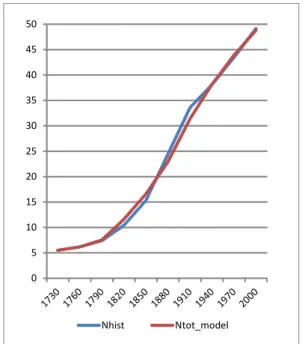
The model is able to reproduce the dynamics of population on the period 1760-1910 as shown by Figure 1, where Nhist is the historical value for total population in England and Ntot_model is the value computed from the model. 0 5 10 15 20 25 30 35 40 45 50 Nhist Ntot_model

(22)

Moreover, it is possible to disentangle the relative eﬀect of technical changes and mortality fall on the evolution of population. We conduct a coun-terfactual analysis eliminating successively the increase in life expectancy, the technological bias, and both of them.

5.2 Life expectancy

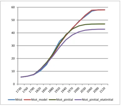
In this section, we successively neutralize the impact of the increase in life expectancy at 50 years old and the decrease in child mortality. Re-sults are presented in Figure 2. Ntot_pinitial is the computed total pop-ulation for a surviving probability at 50 years that keeps its value of 1730. Ntot_pinitial_etatinitial is the computed total population for both the sur-viving probability of young children  and the surviving probability at 50 years  that keep their values of 1730.

0 10 20 30 40 50 60

Nhist Ntot_model Ntot_pinitial Ntot_pinitial_etatinitial

Figure 2: Counterfactual Analysis With no Improvement in Life Expectancy With no increase in life expectancy, neither during childhood nor at 50 years old, the population would have been 10% lower in 1910 and 30% lower in the long run, according to our model.

(23)

5.3 Technological Bias

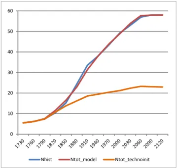
In this section, we neutralize the impact of the technological bias:  keeps its 1730 value.

Figure 3 displays the evolution of the computed population without the technological bias (Ntot_technoinit).

0 10 20 30 40 50 60

Nhist Ntot_model Ntot_technoinit

Figure 3: Counterfactual Analysis with No Technological Bias

The population would have been 40% lower in 1910 with no bias in the technical progress and 60% lower in the long run.

(24)

5.4 Life expectancy and Technological Bias

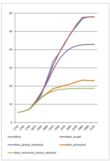
In this section, we neutralize successively the impact of surviving probabili-ties, the impact of the technological bias, and both of them. Results are all depicted in Figure 4 where Ntot_technoinit_pinitial_etainitial stands for total computed population without any increase in surviving probabilities and no technological bias.

0 10 20 30 40 50 60 Nhist Ntot_model Ntot_pinitial_etatinitial Ntot_technoinit Ntot_technoinit_pinitial_etainitial

Figure 4: Total Decomposition: Life Expectancy, Technological Bias, and Both

Population would have been 45% smaller in 1910 and 70% smaller in the long run, without any technological progress and without life expectancy increase. This scenario gives the natural evolution of population for the 1730 parameter values.

(25)

We observe that the major part of population increase from 1730 is due to the technological bias evolution between land and capital.

(26)

6 Conclusion

In this paper, we reproduce the dynamics of population in England since 1760, using an overlapping generations model with endogenous fertility and land. The population growth is driven by a bias technological progress and life expectancy improvement. It is possible to disentangle the relative eﬀect of technical changes and mortality fall on the evolution of population. We conduct a counterfactual analysis eliminating successively the increase in life expectancy and the technological bias. With no increase in life expectancy, population would have been respectively 10% and 30% lower in 1910 and in the long run. The figures would have been respectively 40% and 60% lower, with no bias in the technical progress. Finally, population would have been 45% smaller in 1910 and 70% smaller in the long run, neutralizing both the eﬀect of life expectancy and technological bias. So the major part of population increase is due to the technological bias evolution between land and capital.

7 References

Adjemian S., Bastani H., Juillard M., Karamé F., Maih J., Mihoubi F., Perendia G., Pfeifer J., Ratto M. and Villemot S., 2011, Dynare: Ref-erence Manual, Version 4, Dynare Working Papers, 1, CEPREMAP Aghion P., Howitt P., Murtin F., 2011, "The relationship between health

and growth: when Lucas meets Nelson-Phelps", Institutional Economics. Allen, Robert C., 2009, "Engels’ pause: Technical change, capital

accumu-lation, and inequality in the british industrial revolution," Explorations in Economic History, Elsevier, vol. 46(4), pages 418-435, October. Apps P., Rees R, 2001, "Household production, full consumption and the

costs of children," Labour Economics, Elsevier, vol. 8(6), pp. 621-648, December.

Bargain, Olivier & Donni, Olivier, 2012. "Expenditure on children: A Rothbarth-type method consistent with scale economies and parents’ bargaining," European Economic Review, Elsevier, vol. 56(4), pages 792-813.

Cervellati Matteo and Uwe Sunde, 2005, "Human Capital Formation, Life Expectancy, and the Process of Development", American Economic Review, , 95(5), pp. 1653-1672.

(27)

Crafts Nicholas, 2004, "Productivity Growth in the Industrial Revolution: A New Growth Accounting Perspective", Journal of Economic History, vol. 64 (2), June.

Diamond P., 1965, "Nominal Debt in a Neoclassical Growth Model", Amer-ican Economic Review 55(5), pp. 1126-50.

Dusansky, R., Wilson, P. (1993). - "The Demand for Housing: Considera-tions", Journal of Economic Theory, 61, pp. 120-138.

Galor O., Weil D. N., 2000, “Population, Technology and Growth: From the Malthusian Regime to the Demographic Transition”, American Eco-nomic Review 90 (4), pp. 806-828.

Hansen G., Prescott E., 2002, "Malthus to Solow", American Economic Review 92, No. 4, pp. 1205-1217.

Human Mortality Database, 2015, Available at www.mortality.org or www.humanmortality.de (data downloaded on 22 July 2015). Kongsamut P., Rebelo S., Xie D., 2001, "Beyond Balanced Growth", Review

of Economic Studies 68, pp. 869-882.

Kremer M., 1993, "Population Growth and Technological Change: one mil-lion B.C. to 1990", The Quarterly Journal of Economics 108, pp. 681-716.

Leukhina O., Turnovsky S., 2016, "Push, Pull, and Population Size Ef-fects in Structural Development", Journal of Demographic Economics, Volume 82, Issue 4, December 2016 , pp. 423-457.

Leukhina, Oksana M., and Stephen J. Turnovsky. 2016, "Population Size Eﬀects in the Structural Development of England." American Eco-nomic Journal: MacroecoEco-nomics, 8w(3): 195-229.

Loupias C., Wigniolle B., 2013, "Population, land, and growth", Economic Modelling 31, pp. 223—237.

Maddison A., 2009,The Maddison-Project, http://www.ggdc.net /maddison/historical_statistics/horizontal-file_03-2009.xls.

Maddison A., 2013,The Maddison-Project, http://www.ggdc.net/maddison /maddison-project/home.htm, 2013 version.

(28)

University of Portsmouth, 2015, GB Historical GIS, A Vision of Britain through Time, http://www.visionofbritain.org.uk/unit/10061325 /cube/TOT_POP, data downloaded on 8 December 2015

Wrigley E. A., Schofield R. S., 1989, "The population history of England: 1541-1871", p. 210, Cambridge University Press.

(29)

8 Appendix

8.1

Appendix 1

As the production technology is Cobb-Douglas between  and the other factors, _ = 1_{−  and }_ + _ = . Using equations (26), (27), and (25),

 = ˜1− 1   ˜1− 1   + (1− ) () 1−1 then ˜1− 1   + (1− ) () 1−1 = ˜ 1−1   _ (51)

then from equation (25), ˜ = (1− ) µ  _ ¶ −1 ˜ _ (52)

Thus, we write  as:

= +1  (+1)  1− ()  1− ³ ˜ +1+ +1˜+1+ ˜+1+1 ´ ³ ˜ + ˜+ ˜ ´ As the share of wages  = 1− , ˜= (1− )

³ ˜ + ˜+ ˜ ´ , thus = 0 (1−)  ˜ +1 ˜  and using (52), we get

= 0 (1−)  Ã _ _+1 !  −1 Ã_˜ +1 ˜  ! and so (1 −) =  0  Ã _+1  !  −1 Ã _˜  ˜ +1 ! (53)

(30)

We can also rewrite  and ˜ given by (26) and (27), using (51), thus  =  ˜−1 ∙  _ ¸ −1 ˜  = −   ˜  ∙   ¸ −1

Using equation (53), (32) becomes

_2˜=  Ã +1 _ !  −1 ˜ _˜1−_+1 + ˜

Using equation (53), (33) becomes

+1 = ˜ +1+ ˜+1 ˜   0  Ã _+1 _ ! −1 Ã _˜  ˜ +1 !

Note that from equations (51) and (53), it is possible to recover  and  from  and . = ˜  µ   − 1 ¶  −1µ ₁ 1_{− } ¶  −1 (54) = µ  0  ¶(1−)  Ã _+1 _ !(1−) −1 Ã _˜  ˜ +1 !(1−) (55)

8.2

Appendix 2

TableA1: counterfactual Analysis on Total Population for England

1730 1760 1790 1820 1850 1880 1910 1940 1970 2000 2030 2060 2090 2120 Nhist 5.5 6.2 7.4 10.4 15.3 24.4 33.6 38.1 43.5 49.1 53.0 57.0 58.0 58.0 Ntot_model 5.5 6.2 7.5 11.6 16.6 22.9 31.4 38.1 43.9 48.8 53.9 57.7 57.9 58.0 Ntot_model / Nhist (%) 102 111 108 94 94 100 101 99 102 101 100 100 Ntot_pinitial 5.5 6.2 7.6 11.7 17.0 23.8 31.8 38.8 43.1 45.4 46.6 46.9 47.0 47.0 Ntot_pinitial_etatinitial 5.5 6.2 7.4 11.3 16.2 22.2 28.9 34.7 38.5 40.8 42.1 42.7 42.8 42.9 Ntot_pinitial_etatinitial / Ntot_model (%) 99 98 97 97 92 91 88 84 78 74 74 74 Ntot_technoinit 5.5 6.2 7.4 10.7 13.8 16.2 18.6 19.4 20.4 21.2 22.3 23.3 23.0 23.0 Ntot_technoinit / Ntot_model (%) 98 93 83 71 59 51 46 43 41 40 40 40 Ntot_technoinit_pinitial_etainitial 5.5 6.2 7.3 10.5 13.5 15.8 17.3 18.0 18.4 18.6 18.7 18.7 18.7 18.7 Ntot_technoinit_pinitial_etainitial/ Ntot_model (%) 97 91 82 69 55 47 42 38 35 32 32 32