HAL Id: hal-02861004
https://hal-centralesupelec.archives-ouvertes.fr/hal-02861004
Submitted on 8 Jun 2020HAL is a multi-disciplinary open access archive for the deposit and dissemination of sci-entific research documents, whether they are pub-lished or not. The documents may come from teaching and research institutions in France or abroad, or from public or private research centers.
L’archive ouverte pluridisciplinaire HAL, est destinée au dépôt et à la diffusion de documents scientifiques de niveau recherche, publiés ou non, émanant des établissements d’enseignement et de recherche français ou étrangers, des laboratoires publics ou privés.
Development and assessment of a reduced-order building
model designed for model predictive control of
space-heating demand in district heating systems
Nadine Aoun, Roland Bavière, Mathieu Vallee, Guillaume Sandou
To cite this version:
Nadine Aoun, Roland Bavière, Mathieu Vallee, Guillaume Sandou. Development and assessment of a reduced-order building model designed for model predictive control of space-heating demand in district heating systems. 32nd International Conference on Efficiency, Cost, Optimization, Simulation and Environmental Impact of Energy Systems (ECOS 2019), Jun 2019, Wroclaw, Poland. �hal-02861004�
PROCEEDINGS OF ECOS 2019 - THE 32ND INTERNATIONAL CONFERENCE ON
EFFICIENCY, COST, OPTIMIZATION, SIMULATION AND ENVIRONMENTAL IMPACT OF ENERGY SYSTEMS JUNE 23-28, 2019, WROCLAW, POLAND
Development and assessment of a reduced-order
building model designed for model predictive
control of space-heating demand in district
heating systems
Nadine Aouna, Roland Bavièreb, Mathieu Valléec and Guillaume Sandoud a CEA, Grenoble - CentraleSupélec, Gif-sur-Yvette - ADEME, Angers, France, nadine.aoun@cea.fr, (CA)
b CEA, Grenoble, France, roland.baviere@cea.fr c CEA, Grenoble, France, mathieu.vallee@cea.fr
d CentraleSupélec, Gif-sur-Yvette, France, guillaume.sandou@centralesupelec.fr
Abstract:
This paper presents a control-oriented reduced-order building model intended for optimal management of space-heating demand in district heating systems. The model is designed in accordance with the conclusions drawn from a preliminary study, also presented hereby, evaluating the impact of internal mass and the heating circuit inertia on short-term buildings thermal dynamics. The model parameters identification is carried-out using a hybrid Particle Swarm Optimization – Hooke-Jeeves search algorithm, for three buildings of different energy classes. The algorithm searches for an optimal set of parameters that minimizes the error between the model’s output and historical data generated using a higher order building simulator written in Modelica language. Data used for the identification process is exclusively non-intrusive to the building indoors, and relies solely on measurements available at the substation level. We assess the quality of the identifications per building type. Results showed that the identified models have high prediction ability of the building indoor temperature dynamics, with a maximum absolute error less than 0.7°C. Implementation of optimal predictive space-heating control based on the identified models is in prospect.
Keywords:
District Heating System, Parameters identification, Particle Swarm Optimization, Reduced Order Building Model, Space-heating Demand Flexibility.
1. Introduction
District heating has long been known as an efficient and sustainable mode for space-heating and domestic hot water preparation in dense areas. Optimal management of space-heating demand in district heating systems (DHSs) with prominent attention to buildings’ thermal inertia is seen as a promising technique to shift and shave peak loads, therefore reduce reliance of fossil fuels [1–3]. Model-based optimal predictive control strategies require a reliable building model able to assess and exploit space-heating energy demand flexibility, defined in [4] as the building’s “ability to adapt the energy profile without jeopardizing technical and comfort constraints”. Several studies suggested that thermal demand flexibility is inherently provided within buildings elements, and it is first and
foremost influenced by the envelope insulation level and heat storage capacity [5]. Thus, energy signature models derived from a steady-state energy balance where the building’s space-heating demand is directly correlated with weather conditions without accounting for the thermal capacitance of its envelope [6] are not suitable for optimal control applications. Moreover, in [7], authors concluded that indoor mass is highly influential on buildings thermal dynamics and can increase their time constant by 40%, 25% of which is due to interior partition walls and the remaining 15% is caused by the furniture. Similar conclusions are reported in [8] from a numerical simulation study: addition of furniture to the indoor environment of a lightweight-structure building impacted its transient thermal behaviour and increased its time constant by 43%. On the other hand, heating systems with considerable thermal inertia (radiators, underfloor heating) may as well significantly influence buildings demand flexibility, as demonstrated in [9]. Besides being representative of the building thermal flexibility, a model suitable for optimal control applications at a DHS level needs to be easily derived from non-intrusive, easily accessible data and without detailed description of the buildings geometry, composition or construction materials, for such information is rarely available at a large scale. Therewith, the model shall be control-oriented. Referring to [10,11], a control-oriented model is one with the ability to predict the system’s measured output as a function of its input control variables, as well as its exogenous input signals. Also, all internal states of monitoring interest, for instance the internal air temperature as a comfort indicator in the case of building modelling, must be represented by a model variable. It should efficiently interface with an optimization solver and for an online optimization problem, a control-oriented model should be computationally fast.
Based on the above requirements, we gravitate towards lumped-capacitance Reduced-Order building Models (ROMs). Those are physical models: they are made out of a reduced number of physics-based equations with a few physically interpretable parameters – as opposed to empirical or black-box models. The main assumption behind these models is that several elements of the building system may be aggregated or lumped into a single node and therefore have a uniform temperature. A wide variety of lumped-capacitance ROMs of various orders may be found in the literature [12–16]. The aim of our work is to develop and validate a control-oriented ROM, identifiable at a DHS scale and taking into account all elements that might impact buildings space-heating demand flexibility. This paper is structured as follows. Section 1 introduced the problematic of building modelling for optimal control of space-heating demand at a DHS scale. In section 2 we investigate, via building thermal dynamic simulation, the influence of internal mass and the heating system on space-heating demand flexibility of three buildings from different energy classes commonly found in French DHSs. We present in section 3 a reduced-order modelling methodology, starting by setting-up the model structure based on the preliminary study, and then carrying out parameters identification by minimizing the error between the models output and the output of higher order building simulators using a metaheuristic search algorithm. Application and assessment of the approach’s robustness are presented in section 4. Section 5 concludes the paper.
2. Preliminary study of buildings thermal demand flexibility
2.1. Case-study building simulators
The preliminary study, carried out by thermal dynamic simulation and presented hereby, aims at quantifying the impact of the internal mass and the heating system on space-heating demand flexibility for three buildings of different energy classes. The buildings are simulated in Modelica language. Interested readers may refer to [17] for details about the simulated phenomena and modelling assumptions depicted in Figure 1. In this study the building simulators are parameterized to have the same external geometry. Each simulator covers a 10.85 × 28.21 rectangular footprint area and has only one 2.5 height storey discretized into four thermal zones with surface fractions as shown in Table 1. The building simulators are East – West oriented with = 2⁄ . We assume square-shaped windows, their areas as well as those of opaque constructions per facade are reported in Table 2. This difference between the three building simulators is made through their envelope
construction materials and air renewal rate summarized in Table 3. We relied on Tabula [18], a statistical study on the French residential stock, to set the characteristics of our building simulators.
Figure 1. Spatial discretization of one floor (top view) showing the modelled elements and the thermal phenomena considered in the building thermal dynamic simulator.
Table 1. Common parameters to all building simulators: Percentage of the zones areas to the total floor area.
Night zone Kitchen Day zone Bathroom
35% 15% 40% 10%
Table 2. Common parameters to all building simulators: Areas of opaque constructions and windows per façade.
East facade South facade West facade North facade
Opaque area (m²) 54.30 17.09 45.84 23.60
Glazed area (m²) 16.22 10.04 24.68 3.53
Table 3. Case-study buildings characteristics making them belong to different energy classes. Building
simulator
Envelope Glazing system Number of air renewal per hour
Sizing heating power (kW) 2012 Concrete, exteriorly insulated
with 16 cm of expanded polystyrene Double-glazed with 16 cm of argon 0.3 8.6 1975 Cinderblock, exteriorly insulated with 4 cm of expanded polystyrene Double-glazed with 6 cm of air 0.4 18.5 1915 Stone (40 cm-thick), uninsulated Single-glazed 0.5 35
To represent internal mass, we added four furniture-equivalent slabs inside each zone with properties shown in Table 4. This material assumption is based on [19], a survey on the internal mass and its equivalent heat capacity found in residential and single office buildings in Denmark. The parameter of internal mass per zone area (m in / ) of each slab is the key parameter in the simulator that allows variation of internal thermal mass level. For this study, we consider three internal mass levels:
Light internal mass with a total of 47.5 / . Heavy internal mass with a total of 95 / .
Table 4. Properties of the internal mass equivalent slabs: Thermal conductivity (k), Specific heat capacity (c), Density (ρ), Mass per zone area (m) and thickness (ε).
Material k W m ∙ K⁄ J kg ∙ K⁄ c kg m⁄ρ kg mm ⁄ mm ε Metal 60 450 8000 25 3 Wood / Plastic 0.2 1400 800 25 18 Ceramic / Glass 1.25 950 2000 5 10 Light material 0.03 1400 80 15 120
Light partition walls 0.015 1150 384 25 100
Two classes of heating systems are modelled and can be connected to the building’s thermal zones. The first is an airborne-like system consisting of a direct heat source with an ideal regulation of the internal air temperature constantly maintaining it at its set-point. The second class is a radiator heating system equipped with a thermostatic valve and connected to a centralized production unit. In the case of a building connected to a DHS, this production unit is a substation. In order to assess the impact of the heating system water temperature on buildings short-term thermal dynamics, we consider medium and low temperature radiators. Therefore this study encompasses three heating system:
Airborne. 50°! radiators. 70°! radiators.
2.2. Experimental protocol and thermal demand flexibility index
We first define three mean temperatures:The building mean air temperature:
The building mean walls surface temperature: "#$%&'()
********** =∑#$%&,-#$%&∗ "#$%&/
∑ -#$%& (2)
The building mean perceived temperature, also called operative temperature in [20]: "0)%()12)3
************ = "***** + "'1% **********#$%&'()
2 (3)
The experimental protocol consists of maintaining the building under constant thermal conditions: Constant external temperature ")56 = −11°!.
Constant internal air set-point temperature "'8%#)6 = 19°! in case of an airborne heating system
and "'8%#)6 = 20°! in case of a radiator heating system. The reason for this distinction is to get closely comparable "***** in all cases. In fact a thermostatic radiator valve acts like a '1% proportional controller, in steady-state conditions, if "'8%#)6= 20°!, "***** will be less than 20°!, '1% around 19°!, to allow a constant and stable water mass flow rate through the valve.
No solar radiation.
"'1%
***** = ∑:;<)# -:;<)∗ "'8%:;<)
No internal heat gain.
Then the heating power is cut-off and we observe the system’s free response. For study-cases with airborne heating system (Figure 2 (a)), the heating power is directly cut-off at the zones air node, whereas in case of a radiator heating system (Figure 2 (b)), it is shut-down at the substation level. All three mean temperatures are monitored and the time delays for a 1°! drop in each of these temperatures are registered.
The time delay for 1°! drop in "************, denoted =0)%()12)3 >?, is the building thermal demand flexibility index: a larger =>? means that the heating power may be shut-down for a longer period before 1°! drop is perceived by the consumers, which implies a larger flexibility.
2.3. Results and conclusions
Looking at Figure 2, three observations can be noted:
Within the few minutes following the power cut-off, the air temperature drop is remarkably sharper than the surface temperature drop. This is due to the relatively low thermal inertia of internal air compared to that of the envelope and the internal constructions. Whereof we infer that a ROM of at least second order is required to distinguish these two dissimilar dynamics. After a few minutes, the surface temperature crosses over the air temperature. Heat transfer is
now reversed, given-off by the walls surfaces to heat-up the internal air. This phenomena is sometimes called activation of building thermal mass short-term heat storage [9,21,22]. Notice how air temperature drop gets smoother from this point forward. The drop velocity of air, surface and their average perceived temperature becomes uniform and only on the long run the building system seems to behave as a first-order system.
When comparing airborne to radiator heating systems, we observe that the heating power from the latter decreases gradually after the cut-time, owing to the thermal inertia of the heating system itself (piping and heating water). This leads to overall slower temperature drops.
Results of =>? are displayed in Figure 3. They allow a quantitative comparison of all 27 cases: In the well-insulated building with heavy internal mass, an airborne heating system yielded
longer =>? than radiator heating systems in the equivalent empty building, contrary to the two Figure 2. 2012 lightly furnished building’s thermal response following space-heating power cut-off:
other building classes. Therefore we conclude that internal mass is particularly influential on short-term thermal dynamics of buildings with high thermal insulation levels.
On average, buildings with 70°! radiators had 35% longer =>? than those with 50°! radiators.
The lower the insulation level, and the lower the internal mass level, the higher is the sensitivity towards heating water temperatures.
From a control point of view, we recall that =>? give an order of magnitude of how long the
heating system could be set-back before the 1°! drop is perceived by a consumer, in extreme conditions (−11°!). Interestingly, according to our simulator, average values of these =>? are:
▫ More than an hour for a well-insulated building (2012). ▫ 20 minutes for a building of medium insulation level (1975). ▫ 10 minutes for an uninsulated building (1915).
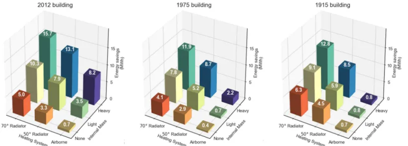
We simulated again all cases to find out the amount of energy that would have been consumed during =>? but without the power cut-off. Despite the large difference in =>? among buildings from different energy classes, energy savings turned out to be quite comparable (Figure 4).
Figure 3. 1°C drop delays in perceived temperature, =>? (min).
3. Reduced-order building modelling
3.1. Model structure
Based on the preliminary study, we propose the ROM structure given by the system of equations (4) through (10), also represented in Figure 5.
The building itself is linearly modelled with three power balance equations ((4) to (6)) around three temperature nodes with associated thermal capacitances: one for the indoor air, another for the internal mass exchanging heat solely with the indoor air and, lastly, one for the external envelope exchanging heat with both the outdoor and the indoor air. Additionally, direct ventilation and infiltration heat losses to the exterior are accounted for in the indoor air power balance equation. Solar gain is also linearly modelled and injected into each of these nodes. The building model, apart from the solar gain model, is quite similar to the one investigated in [14] which proved to be sufficiently accurate, with a slight difference: the indoor air temperature node in [14] is assumed to be capacitance free. Indeed, its capacitance is rather negligible relatively to the two other capacitances in the model. The heating system model (equations (7) and (8)), operating in closed loop, is non-linear and features two temperature nodes with associated thermal capacitances: one for the emitter delivering heat to the indoor air and another for the heating circuit drawing heat from the substation. The non-linearity appears in the heat exchange between these two nodes resulting from the product between the mass flow rate and their temperature difference. Equations (9) and (10) are the closed loops proportional regulation equations, with saturation (BCDE? means the bounded value of C between 0 and 1).
Thus, the model has 5 states (temperatures at the nodes) and 2 outputs, calculated at each time step by solving the 7-equations system. From a DHS operator point of view, the only controllable input to this model is "(8%#)6 ("'8%#)6 being controlled by the consumers). The measured outputs at the substation are ΦGGH and I . They will be used to identify the 16 model parameters, marked in a bold font.
JKLM∙N"'8%NO = PQ∙ ")56− "'8% + PL∙ ")<2− "'8% + PR∙ "S'##− "'8% + PT∙ ")S− "'8% + UKLMV ∙ W#;X (4) JYZQ∙N"NO = P)<2 [∙ ")56− ")<2 + PL∙ "'8%− ")<2 + UYZQV ∙ W#;X (5) JRKVV∙N"NO = PS'## R∙ "'8%− "S'## + URKVVV ∙ W#;X (6) J\LM∙N"(8%NO = Z]∙ ΦGGH+ I ∙ ^0∙ ")S− "(8% (7) JYR∙N"NO = I ∙ ^)S 0∙ "(8%− ")S + PT∙ "'8%− ")S (8) ΦGGH= ΦGGHS'5∙ _` \LM a ∙ "(8%#)6− " (8% bc? (9) I = IS'5∙ _` KLM a ∙ "'8%#)6− "'8% b c ? (10)
Figure 5. Schematic representation of the proposed reduced-order model structure.
Solar gain model
Heating system model
Heat flow Mass flow Signal flow
3.2. Parameters identification
Given the ROM structure, parameters identification aims at finding the optimal set of 16 parameters that minimizes the objective function d formulated in (11). d is the integral over the training period (December 12th to the 31st) of the weighted quadratic errors between the ROM outputs ( Iefgand
ΦGGHefg) and those of the higher order building simulator ( I#8Sand Φ
GGH#8S), both subject to the same
inputs (")56, W#;X, "'8%#)6 and "(8%#)6). The building simulator data is generated at a sampling time of 5 minutes under the following conditions:
"(8%#)6 is linked to ")56 with a heating curve and it is reduced during night-time as a form of power
set-back to stimulate the thermal dynamics of the heating system and therefore enhance the identifiability of its parameters. The settings of the heating curve depend on the building energy class: the lower the energy consumption, the lower is the heating water temperature.
"'8%#)6 = 20°! in all zones, at all times. In fact, "
'8%#)6 is not a controllable input and its value might
be variable. However, the building simulator includes a stochastic internal gain model which is assumed to aggregate all the uncertainties of the building system.
Unlike other works [12,14,16], the parameters identification objective function d does not feature the internal air temperature signal, since we consider it to be intrusive and not guaranteed to be available at a DHS scale. Instead, we relied on I which is proportionally linked to the unmeasured "'8% in the ROM and therefore might be regarded as its image. To ensure that the ROM well-predicts "'8%, the error on I is double-weighted with respect to that on ΦGGH.
The minimization of d is performed using the optimization software GenOpt [23]. GenOpt is conceived to optimize computationally expensive objective functions assessed by an external simulation tool. We used Dymola to implement the ROM model and calculate d, given the building simulator data and parameters that are iteratively tested by GenOpt, based on previous trails dictated by a search algorithm. We selected a hybrid metaheuristic algorithm that starts with a Particle Swarm Optimization on a coarse mesh of 150 generations of 150 particles each, and then refines the search results with a Hooke-Jeeves pattern search. The search is reasonably initialized by physically estimating the parameters, and normalized with respect to the initial values. The normalized search space is then limited between 1/3 and 3 for each parameter.
4. Methodology application and assessment
OOIn this section, we apply the parameters identification approach to infer a ROM for each of the three case-study buildings introduced in section 2.
Beforehand, we generated two sets of data per building: the first is from December 12th to 31st for the training
phase, and the second is from January 6th to 25th to assess
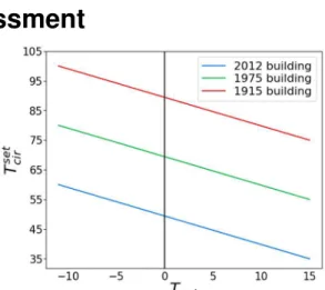
the models prediction ability. A typical meteorological year weather file for the city of Grenoble is used during the simulations. The heating curves used during normal operation for the three buildings are plotted in Erreur !
Source du renvoi introuvable.. During the night-time,
"(8%#)6 is limited to 35°!, 55°! and 75°! for the 2012,
1975 and 1915 building, respectively. We recall that all buildings have different envelops with the same
d = h i23 ∙ j I#8SI− IS'5efgk +13 ∙ jΦGGH#8SΦ− ΦGGHefg ##6 S'5 k l 3)( ?#6 3)( ? 6n NO (11)
Figure 6. Heating curves used to set the heating water temperature (out of night-time set-back).
geometry, the same amount of internal mass (heavy) and the same internal gain signal.
GenOpt converges to the identified parameters listed in Table 5 after about 25k simulations, taking around 25 minutes on an 18-core, 36-thread processor machine. We notice that the minimal value of d for the 2012 building is the highest among the others. This is due to the sensitivity of this building class towards internal heat gain accounting for about 20% of its space-heating sizing power (Figure 7), which is not modelled in the ROM. To compensate the effect of internal gain, the search algorithm might find biased parameters: over-estimated solar gain coefficients and under-estimated heat loss coefficients. This leads to larger errors in periods of low internal gain.
Table 5. Identified parameters and minimal objective-function value for all case-study buildings. Identification results 2012 building 1975 building 1915 building
JKLM Bo p⁄ D 2.88E+07 2.95E+07 1.78E+07
JYZQ Bo p⁄ D 9.60E+08 2.31E+08 1.95E+09
JRKVV Bo p⁄ D 1.94E+08 6.44E+05 1.50E+07
J\LM Bo p⁄ D 1.55E+04 1.22E+04 1.14E+04
JYR Bo p⁄ D 8.25E+03 2.25E+03 5.20E+02
PQ Bq p⁄ D 232.5 346.5 555 PL Bq p⁄ D 27.3 361.1 1125 P[ Bq p⁄ D 1720 960 1200 PR Bq p⁄ D 3510 2200 3360 PT Bq p⁄ D 375 505 450 UKLMV B D 14.1 7.20 13.2 UYZQV B D 14 4.83 1.75 URKVVV B D 6.5 2.95 2.9 Z] B−D 0.96 0.99 0.83 `\LMa B1 p⁄ D 0.57 0.29 0.35 `KLMa B1 p⁄ D 0.52 0.43 0.48 d B−D 3509.53 2444.47 1339.03
Figure 7. Proportions of the internal heat gain and the substations space-heating power. The first criterion to assess the models reliability is its ability to fit certain variables of interest. Here we are interested in predicting the output signals and the indoor air temperature. We define the fit function of a variable C in (12) and evaluate its value over the training and the prediction periods. Note that for the variable "'8%, "'8%#8S is the mean zones temperature weighted by the zones floor area, it is denoted "******, and "'1%#1S '8%S'5 = "'8%#)6 = 20°!. Results are shown in Table 6. For all variables of all buildings, the fit is slightly deteriorated during the prediction phase, but remains acceptable. Besides, the error range of Tstu given in Table 7 shows that the maximum absolute error between the simulator and the model is less than 0.7°! for the 2012 building, and less than 0.5°! for the 1915 building during the prediction phase, making the models sufficiently reliable for control applications.
Table 6. Assessment of the models variables fit during the training and the validation phases. Assessed variable Phase 2012 building 1975 building 1915 building
ΦGGH Training 93.75% 92.27% 93.64% Prediction 89.08% 87.78% 89.23% I Training 90.57% 94.95% 95.92% Prediction 83.20% 91.38% 87.75% "'8% Training 88.67% 83.56% 92.73% Prediction 80.73% 73.20% 82.70%
Table 7. Assessment of the models "'8%.error ranges.
Assessed variable Phase 2012 building 1975 building 1915 building Error range of
,"'8%efg− " '1%#1S
******/ °! Training Prediction [-0.23, 0.33] [-0.35, 0.64] [-0.52, 0.13] [-0.51, 0.26] [-0.22, 0.22] [-0.46, 0.25] The second criterion is the physical relevance of the building equivalent heat loss coefficient which may be calculated from the identified parameters using (13), and estimated from the building sizing data using (14), with ")56#8:8<v= −11°! in Grenoble. Table 8 shows good consistency between w)x83)<6 and w)x)#68S for all buildings.
Table 8. Identified and estimated heat loss coefficients.
Equivalent heat loss coefficient 2012 building 1975 building 1915 building w)x83)<6 Bq/pD 259.37 608.90 1135.65
w)x)#68S Bq/pD 277.42 596.77 1129.03
5. Conclusion
In this paper, we studied the influence of internal mass and heating systems on space-heating demand flexibility of buildings from different energy classes. We concluded that internal mass is mostly influential in well-insulated buildings and can stretch their temperature drop delay to over an hour. Poorly-insulated buildings are rather sensitive to the heating system temperature level and despite having shorter temperature drop delays, they offer considerable energy savings during brief power set-backs. We went on to designing a reduced-order building model featuring a thermal capacitance representing the internal thermal mass, with a non-linear heating system model. Then we proposed a parameters identification approach which aims at minimizing the non-intrusive model outputs found at the substation level using metaheuristic optimization, hence making the strategy applicable at a district heating scale. We applied the methodology on three case-study buildings. Assessment of the identification results and the models prediction ability showed that they are sufficiently reliable and may be used for space-heating optimal control applications in up-coming work.
dyO C = j1 − z{ j1, }******************************CCefgS'5 − C− C#1S#1S}kk × 100 (12) w)x83)<6= w8∙ w;+ w;∙ w2+ w2∙ w8 w8 + w; (13) w)x)#68S = ΦGGH S'5 "'8%#)6− " )56#8:8<v (14)
Acknowledgments
We gratefully acknowledge ADEME (Agence de l'Environnement et de la Maîtrise de l'Énergie) for their financial support in funding the PhD thesis of Nadine Aoun.
Nomenclature
Acronyms
DHS District Heating System ROM Reduced-Order Model
Letter symbols
^0 specific heat capacity of the heating water, J/(kg K)
J thermal capacitance, J/K
`~ gain of a proportional temperature regulator, 1/K
UV Solar gain coefficient, m²
I mass flow rate, kg/s
Z] efficiency coefficient of the heating system
" temperature, K
PT heat exchange coefficient between the indoor air and the heat emitters, W/K
PL heat exchange coefficient between the indoor air and the envelope, W/K
PR heat exchange coefficient between the indoor air and the internal mass, W/K
P[ heat loss coefficient through the envelope, W/K
PQ heat loss coefficient due to ventilation, W/K
Greek symbols
=>? space-heating demand flexibility index – Time delay for 1°! drop in "************ 0)%()12)3
W#;X global horizontal solar radiation flux, W/m²
Φ••€ space-heating power at the substation, W
Subscripts Superscripts
•y‚ building indoor air •C maximum threshold ^y‚ heating circuit ƒ„O set-point temperature
„ heat emitter ƒy thermal dynamic building simulator „{… building envelope
•ƒƒ building internal mass
References
[1] Guelpa E, Verda V. Optimization of the Thermal Load Profile in District Heating Networks through “Virtual Storage” at Building Level. Energy Procedia 2016;101:798–805. doi:10.1016/j.egypro.2016.11.101.
[2] Kensby J, Trüschel A, Dalenbäck J-O. Potential of residential buildings as thermal energy storage in district heating systems – Results from a pilot test. Appl Energy 2015;137:773–81. doi:10.1016/j.apenergy.2014.07.026.
[3] Leśko M, Bujalski W. Operational optimization in district heating systems using thermal inertia of buildings. Rynek Energii 2016.
[4] Reynders G, Amaral Lopes R, Marszal-Pomianowska A, Aelenei D, Martins J, Saelens D. Energy flexible buildings: An evaluation of definitions and quantification methodologies applied to thermal storage. Energy Build 2018;166:372–90. doi:10.1016/j.enbuild.2018.02.040.
[5] Foteinaki K, Li R, Heller A, Rode C. Heating system energy flexibility of low-energy residential buildings. Energy Build 2018;180:95–108. doi:10.1016/j.enbuild.2018.09.030.
[6] Rabl A, Rialhe A. Energy signature models for commercial buildings: test with measured data and interpretation. Energy Build 1992;19:143–54. doi:10.1016/0378-7788(92)90008-5.
[7] Antonopoulos KA, Koronaki EP. Effect of indoor mass on the time constant and thermal delay of buildings. Int J Energy Res 2000;24:391–402. doi:10.1002/(SICI)1099-114X(200004)24:5<391::AID-ER585>3.0.CO;2-L.
[8] Johra H, Heiselberg P, Dréau JL. Influence of envelope, structural thermal mass and indoor content on the building heating energy flexibility. Energy Build 2019;183:325–39. doi:10.1016/j.enbuild.2018.11.012.
[9] Le Dréau J, Heiselberg P. Energy flexibility of residential buildings using short term heat storage in the thermal mass. Energy 2016;111:991–1002. doi:10.1016/j.energy.2016.05.076.
[10] Kircher KJ, Max Zhang K. On the lumped capacitance approximation accuracy in RC network building models. Energy Build 2015;108:454–62. doi:10.1016/j.enbuild.2015.09.053.
[11] Rubio-Herrero J, Chandan V, Siegel C, Vishnu A, Vrabie D. A Learning Framework for Control-Oriented Modeling of Buildings. 2017 16th IEEE Int. Conf. Mach. Learn. Appl. ICMLA, 2017, p. 473–8. doi:10.1109/ICMLA.2017.00079.
[12] Berthou T, Stabat P, Salvazet R, Marchio D. Development and validation of a gray box model to predict thermal behavior of occupied office buildings. Energy Build 2014;74:91–100. doi:10.1016/j.enbuild.2014.01.038.
[13] Fraisse G, Viardot C, Lafabrie O, Achard G. Development of a simplified and accurate building model based on electrical analogy. Energy Build 2002.
[14] Harb H, Boyanov N, Hernandez L, Streblow R, Müller D. Development and validation of grey-box models for forecasting the thermal response of occupied buildings. Energy Build 2016;117:199–207. doi:10.1016/j.enbuild.2016.02.021.
[15] Vivian J, Zarrella A, Emmi G, De Carli M. An evaluation of the suitability of lumped-capacitance models in calculating energy needs and thermal behaviour of buildings. Energy Build 2017;150:447–65. doi:10.1016/j.enbuild.2017.06.021.
[16] Reynders G, Diriken J, Saelens D. Quality of grey-box models and identified parameters as function of the accuracy of input and observation signals. Energy Build 2014;82:263–74. doi:10.1016/j.enbuild.2014.07.025.
[17] Aoun N, Bavière R, Vallée M, Brun A, Sandou G. Dynamic simulation of residential buildings supporting the development of flexible control in district heating systems. 13th Int. Model. Conf., Regensburg, Germany: 2019.
[18] ADEME, EPISCOPE. TABULA. France: 2015.
[19] Johra H, Heiselberg P. Influence of internal thermal mass on the indoor thermal dynamics and integration of phase change materials in furniture for building energy storage: A review. Renew Sustain Energy Rev 2017;69:19–32. doi:10.1016/j.rser.2016.11.145.
[20] Auliciems A, Szokolay SV, Passive and Low Energy Architecture International, University of Queensland, Department of Achitecture. Thermal comfort. Brisbane: PLEA; 1997.
[21] Wolisz H, Block P, Streblow R, Müller D. Dynamic activation of structural thermal mass in a multi-zonal building with due regard to thermal comfort. 14th Int. Conf. Int. Build. Perform. Simul. Assoc. Hyderabad India, 2015.
[22] Olsthoorn D, Haghighat F, Moreau A, Lacroix G. Abilities and limitations of thermal mass activation for thermal comfort, peak shifting and shaving: A review. Build Environ 2017;118:113–27. doi:10.1016/j.buildenv.2017.03.029.
[23] Wetter M. GenOpt (R), Generic Optimization Program, User Manual, Version 3.1.1. Lawrence Berkeley National Laboratory: Berkeley, CA, USA; 2016.