Morphorider: a new way for Structural Monitoring via the shape acquisition with a mobile device equipped with an inertial node of sensors

(1)

HAL Id: hal-01962789

https://hal.inria.fr/hal-01962789

Submitted on 21 Dec 2018

HAL is a multi-disciplinary open access archive for the deposit and dissemination of sci-entific research documents, whether they are pub-lished or not. The documents may come from teaching and research institutions in France or abroad, or from public or private research centers.

L’archive ouverte pluridisciplinaire HAL, est destinée au dépôt et à la diffusion de documents scientifiques de niveau recherche, publiés ou non, émanant des établissements d’enseignement et de recherche français ou étrangers, des laboratoires publics ou privés.

Morphorider: a new way for Structural Monitoring via

the shape acquisition with a mobile device equipped

with an inertial node of sensors

Tibor Stanko, Nathalie Saguin-Sprynski, Laurent Jouanet, Stefanie Hahmann,

Georges-Pierre Bonneau

To cite this version:

Tibor Stanko, Nathalie Saguin-Sprynski, Laurent Jouanet, Stefanie Hahmann, Georges-Pierre Bon-neau. Morphorider: a new way for Structural Monitoring via the shape acquisition with a mobile device equipped with an inertial node of sensors. EWSHM 2018 - 9th European Workshop on Struc-tural Health Monitoring, Jul 2018, Manchester, United Kingdom. pp.1-11. �hal-01962789�

(2)

9th European Workshop on Structural Health Monitoring July 10-13, 2018, Manchester, United Kingdom

Morphorider: a new way for Structural Monitoring

via the shape acquisition with a mobile device

equipped with an inertial node of sensors

Tibor Stanko1,2, Nathalie Saguin-Sprynski1, Laurent Jouanet1, Stefanie Hahmann2, and Georges-Pierre Bonneau2

1 CEA, LETI, MINATEC Campus, Université Grenoble Alpes, Nathalie.saguin@cea.fr 2 Université Grenoble Alpes, CNRS (Laboratoire Jean Kuntzmann), INRIA,

stefanie.hahmann@inria.fr

Abstract

We introduce a new kind of monitoring device, allowing the shape acquisition of a structure via a single mobile node of inertial sensors and an odometer. Previous approaches used devices placed along a network with fixed connectivity between the sensor nodes (lines, grid). When placed onto a shape, this sensor network provides local surface orientations along a curve network on the shape, but its absolute position in the world space is unknown. The new mobile device provides a novel way of structures monitoring: the shape can be scanned regularly, and following the shape or some specific parameters along time may afford the detection of early signs of failure. Here, we present a complete framework for 3D shape reconstruction. To compute the shape, our main insight is to formulate the reconstruction as a set of optimization problems. Using discrete representations, these optimization problems are resolved efficiently and at interactive time rates. We present two main contributions. First, we introduce a novel method for creating well-connected networks with cell-complex topology using only orientation and distance measurements and a set of user-defined constraints. Second, we address the problem of surfacing a closed 3D curve network with given surface normals. The normal input increases shape fidelity and allows to achieve globally smooth and visually pleasing shapes. The proposed framework was tested on experimental data sets acquired using our device. A quantitative evaluation was performed by computing the error of reconstruction for our own designed surfaces, thus with known ground truth. Even for complex shapes, the mean error remains around 1%.

1. Introduction

1.1 Shape capture via MEMS

Traditionally, digital models of real-life shapes are acquired with 3D scanners, providing point clouds for surface reconstruction algorithms. However, there are situations when 3D scanners fall short, e.g. in hostile environments, for very large or deforming objects. In the last decade, alternative approaches to shape acquisition using data from microsensors have been developed (1, 2). The use of cheap and miniature inertial microsensors is common in many domains. Traditionally, they are at the heart of navigation systems to control aircrafts, satellites or unmanned vehicles. Only recently, the use of inertial sensors for curve and surface reconstruction has emerged. The novelty of this reconstruction problem is to deal purely with orientation and distance data instead of point clouds traditionally acquired using optical 3D scanners. While a few

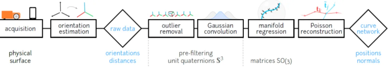
2. Acquisition device

In this section we describe the Morphorider, a novel MEMS based mobile device, which is used for data acquisition. The key idea is to provide a device which can trace an unconstrained virtual network of curves on the scanned surface. This enables acquisition and reconstruction of a broader family of shapes than existing fixed-topology devices. 2.1 Sensors of orientation

To measure the orientation of the device, we use inertial sensors able to provide their rotation with respect to a measured field. Concretely, we use: a 3-axis accelerometer providing the angle with respect to the Earth’s gravity field when static (the vertical direction); and a 3-axis magnetometer providing the angle with respect to the Earth’s magnetic field, as long as no external magnetic source disturbs the measurement. An orthonormal frame that represents the 3D orientation is determined by combining the

(4)

information from both sensors. The sensors are placed in the device so that one of the axes of the orthonormal frame is aligned with the motion axis. The orientation of the node is estimated from sensor measurements by solving the Wahba’s problem using SVD (5,6).

2.2 Sensor of displacement

Orientations are by themselves not sufficient to reconstruct the spatial locations, we also need to know the displacement of the device along the scanned curves. To this end, we use an odometer: the encoder disk sends a tick when 1/500 of a round is traveled. The displacement of the Morphorider has to be controlled to avoid slidings.

2.3 Data collection

The Morphorider is an autonomous Bluetooth mobile node. A microcontroller managed by a software driver (allowing to communicate with the device) reads sequentially the sensors data (values from odometer and inertial sensors) via a serial bus. Morphorider is equipped with a battery and communicates with the host computer by Bluetooth.

2.4 Acquisition process

We use a MATLAB interface to acquire data. In addition to measuring the orientations and distances along curves, we also specify the network topology: prior to acquisition, we assign a unique index between 0 and n − 1 to each of the n network nodes (intersections). The acquisition is controlled remotely using a wireless numpad (Fig. 1). When starting a new curve, we first indicate if the curve is at the boundary or in the interior. Then, every time the device passes through a node, we record its index. To handle surfaces with boundary, we require the user to tag all boundary segments.

Figure 1. Morphorider and the wireless keypad used for marking nodes during acquisition.

3. Mathematical resolution

(5)

The Morphorider provides orientations and distances along a network of smooth curves on a surface. We will now use these data to reconstruct the network: this network is then interpolated with surfacing methods detailed in next section. Fig. 2 illustrates the different steps of the method.

Figure 2. Curve network steps 3.1.1 Problem formulation

We consider a collection Γ of G1 smooth curves embedded on a 2-manifold surface S ⊂ R3. Denote by x: [0,L] → R3 the natural parametrization of γ ∈ Γ where L is the length of γ. For a fixed point x on the curve, the orthonormal Darboux frame D = (T,B,N) consists of the unit tangent vector T = �, the outward surface normal N, and the binormal B = N × T (7). We represent the Darboux frame D as an orientation matrix A = [T B N] which is a member of the special orthogonal group SO(3). Knowing the topology of network and a set of orientations �! = �(� �! ) sampled at known

distances �! ∈ [0,L] for each curve γ, the goal is to retrieve the unknown positions x. 3.1.2 Pre-filtering

The noisy raw data are first preprocessed to obtain a uniform sampling with respect to arc-length. In this step, we use unit quaternions to represent the orientations; see (8) for details and conversion relations. First, we remove the outliers and the duplicate measures; we then fix the sampling distance ℎ!"# and compute uniform distance

parameters �! = �ℎ for each curve γ with length L, where h = L/N and N =

round(L/ℎ!"#). The corresponding unit quaternion �� is computed by convoluting the

measured orientations with a Gaussian kernel: �!= mean !!∈! �_!,!_�_!, �_!,! _{= �� −}1 2 �_!_{− �}_! �ℎ_!"# !

The parameter σ ∈ [0.2, 0.5] controls the radius of convolution. Means are computed using the q method (8).

3.1.3 Filtering by regression on SO(3)

The next step is to smooth the orientations and ensure the consistency of surface normals at intersections of curves. To this end we use a variant of smoothing splines on the manifold SO(3). Recall that a smoothing spline x: [t0, tN] → Rn for a set of points pi

∈ Rn minimizes the energy

� �_! _{− �}_! !+ � � ! !! !_! ! !!! + � � !��

The weights � and µ > 0 control stretching and bending of the spline, respectively. We will write this energy as E = E0 + � E1+µ E2. Similarly, smoothing splines have been

(6)

defined for data on Riemannian manifolds (9). To smooth the orientation data Ai on the

manifold SO(3), we use the following energies (see (10) for details): �! � = !_!!! ��− �! _!!, �! � = ! ! ��− �!!! ! ! !!! !!! , �! � = ! !! ��_(�_��_(� �!�+ �!!!)) _! ! !!! !!! .

In our setup, the raw data Ai is associated to a network Γ and the above energy terms are

summed over all curves γ ∈ Γ. Simultaneously with regression on SO(3), we solve the consistency constraints as follows. Let �!, �! be the local Darboux frames of two curves

at their intersection. Then the two frames are called consistent if �� is obtained by

rotating �! around the surface normal. Denote by N the set of all such pairs (�!, �!). To

enforce consistency, we add a term penalizing the difference in projection on the normal component

�! Γ = �!|� − �� |� ! (�!,�!)∈!

The final energy is minimized using Riemannian trust region algorithm (11).

3.1.4 Integration

The positions x are computed by solving Poisson’s equation Δx = ∇·T where T is the tangent field extracted from the filtered orientations X. The differential operators are discretized via finite differences: ��=

�

��(��!�− ��+ ��!�), ∇��= �

�(��− ��!�).

The above discretization is valid for all interior vertices. At endpoints of open curves, we directly impose the boundary conditions �

� ��− �� = ��, �

� ��− ��!� = ��.

The resulting linear system LX = T is sparse with at most three non-zero coefficients per row.

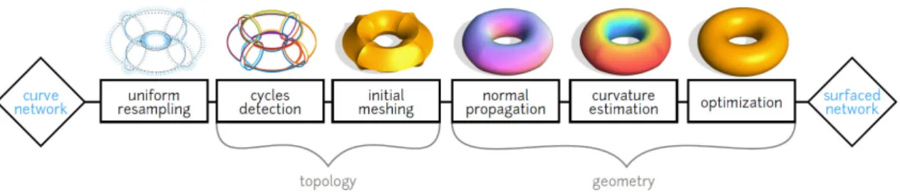
3.2 Reconstruction of the surface

3.2.1 Overview of the method

We use the following pipeline to generate a globally smooth surface from curve and normal vector input:

1. Raw data are first interpolated with cubic splines and resampled uniformly. We efficiently detect the network cycles, then triangulate them in plane.

2. By solving two biharmonic systems with boundary constraints, we both propagate the surface normal and obtain an initial guess for the vertex positions; this allows us to compute discrete mean curvature for the whole mesh.

3. Finally, we solve a linear optimization problem computing a surface that best matches the mean curvature vector formed by the mean curvature value and the normal computed in the previous step.

(7)

Figure 3. Surfacing steps from a curve network. 3.2.2 Exploiting local tangent space to detect cycles

The detection of cycles in a general curve network is a complex and ambiguous problem, often without a unique solution. In order to overcome this problem, methods for surfacing sketched networks adopt a variety of heuristics to mimic the human perception (12). In our specific setting, due to the assumptions on surface smoothness and manifoldness, and the availability of the oriented normals, any possible ambiguity can be efficiently resolved as follows. A segment is a portion of curve bounded by two adjacent nodes. A cycle is a set of adjacent segments which constitute a boundary of some surface patch; the curve cycles are assumed to be contractible on S. Our algorithm is inspired by face extraction in edge-based data structures for manifolds. First, the segments adjacent to any node are cyclically sorted with respect to the orientation given by the input normal at that node. Then, starting from any (Node, Segment) pair, we trace a unique cycle by choosing the next node as the other endpoint of the current segment. The next segment is then picked from the ordered set.

3.2.3 Network tessellation

We represent the surface S as a triangle mesh M = (V,F) with vertices V and faces F. Prior to the tessellation, the positions pi and normals ni along the curve network C are

interpolated with cubic splines and resampled with arc length parameterization, providing a uniformly sampled network. Each cycle defines a closed 3D curve Γ bounding an n-sided surface patch. We triangulate a planar projection of each cycle individually to obtain the topology F of the whole mesh; the triangulation is computed using Shewchuk’s Triangle (13). The plane of projection for each cycle is defined by the average position � and average unit normal � computed from resampled Γ.

Even though this simple planar projection is not necessarily injective, we have found that it leads to a much smaller distortion between the planar triangulation and the mesh triangulation, in comparison with other planar embeddings of Γ with guaranteed injectivity (e.g. mapping to a circle or a polygon). Notice that a more robust but time-consuming 3D curve tessellation method can be used (14).

3.2.4 Variational smoothing

At this point of the process we have computed the topology F of the mesh M, and we have the constraints – positions and normals – for vertices along the resampled curve network C. In this section, we describe a variational method for computing the positions of the free vertices, based on the discretization of the Laplace-Beltrami operator and of the mean curvature vector for piecewise linear surfaces.

Discretization of Δ. Given a piecewise-linear function _{�� = �(�}�) defined over the

(8)

∆� �� = �� ,�(��− ��) �∈�_�(�)

where N1(i) is the index set of 1-ring neighborhood of vi. The vertex weights are stored in the diagonal mass matrix Mii = 1/wi, while the edge weights ��,� are stored in a

symmetric matrix Ls (��)_�,� = − �_�� ∈�_� � , _{� = �} �_��, _{� ∈ �}_� � �, ��

The discrete Laplace operator is then characterized by the matrix L = M-1Ls. In the following, we use the cotangent Laplacian wi = 1/Ai, wi j = 1/2(cot(αi j)+ cot(βi j)) where αi j and βi j are the two angles opposite to the edge (i,j), and Ai is the Voronoi area of vi (16).

Initial vertices and propagated normals. Let Vc denote the set of vertices lying on the

curve network C, and Vf denote the remaining free vertices. We start by computing

initial positions and initial normals for all vertices by solving two biharmonic systems: ��∗ _{= � for positions and �}�_�∗ _{= � for normals. The propagated normals N* are then} normalized. We choose L as the cotangent Laplacian based on the planar triangulation computed in the previous section. The positional and normal boundary conditions are incorporated into the systems as hard constraints by eliminating the corresponding rows of the matrix L2 as described in (17).

Mean curvature guide. From the initial vertices v* and the propagated normals n* we now compute mean curvature information that will guide the optimization. Following Sullivan (18), the discrete mean curvature vector at a mesh vertex v is proportional to the integral of the conormal η = n × e, i.e. the vector product of the normal and the unit tangent to the boundary, �� = _��

� , computed along the boundary of the

1-neighborhood N1 of v. Sullivan evaluates this integral using the triangle normals defined

by the mesh vertices v. In order to take the input data into account, we evaluate this integral using the propagated normals n* rather than the triangle normals. More precisely, we compute the mean curvature vector for the initial surface by summing the contributions for all oriented edges opposite to v*:

� �∗ ₌ � � �∗+ �_�∗+ � �!� ∗ �∗+ �_�∗+ � �!� ∗ ×(��!� ∗ _{− �} � ∗₎ �!� �!�

where n* denotes the propagated normal at the vertex

v* of valence n, whose Voronoi area is A and its

neighbors are ��∗ (indices taken modulo n, see inset).

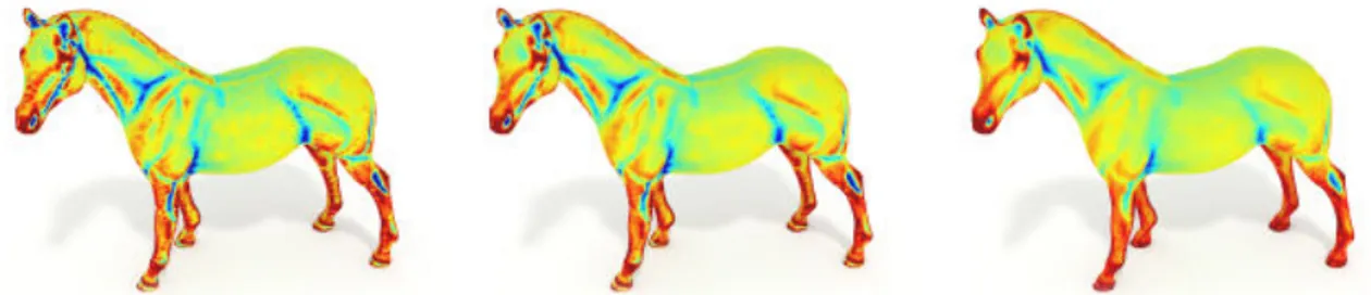
This formula for computing the mean curvature is a key part to our method. Its originality lies in blending together the positional information (the initial vertices v*) with the additional normal information (the propagated normal n*) not directly inferred from the positions. In contrast, the usual discrete mean curvature formulations, such as

(9)

Figure 4, where we show three discrete mean curvatures, one based on (16) (left), and two on our formula (middle and right) computed with the same geometry, but using two different normal fields. It can further be observed in Figure 2 that our mean curvature measure behaves at least as well as the standard measures even with a low quality mesh. Since we apply the mean curvature formula in this paper to good quality triangulations resulting from a planar Delaunay tessellation we did not investigate the incorporation of propagated normals into more robust discrete mean curvature measures.

Figure 4. Mean curvature of the irregular horse mesh with 3 different computations.

Optimization. We can now define the energy functional � (�) = �∈� ∆� + � � �∗ � with �(�) = �(�) being the scalar mean curvature at v. This formulation, derived from the well-known formula Δv = -h n, enables us to match the mean curvature and the propagated normals. In order to exactly interpolate the positional constraints Vc, we

perform the following optimization:

�� . �. � = �∗ �� ∈ ��

The energy E is written in matrix form as � � = �� − �� _{and minimized by}

solving �� = �� _�∗ with = �� , � = �_� �

� , where � is the matrix of Lagrange multipliers, �� is the

�×� identity matrix, and H is the matrix of propagated normal N* scaled by the mean curvature h.

4. Results

Fig. 5 shows an illustration of the process applied to a specifically designed shape with known ground truth. The surface of the lilium is scanned by acquiring orientations along curves using the Morphorider (left). Four images present the successive steps of the reconstruction process: naive integration of the scanned data fails to close the network (middle left); reconstructing the network by solving a Poisson system resolves topological problems but yields noisy and inconsistent normals (middle); filtering orientations prior to Poisson reconstruction gives a consistent network (middle right) available for surface fitting (right).

(10)

Figure 5.Process of surface reconstruction illustrated by results on a real shape.

Concerning convergence considerations, the reconstruction error for the acquired networks is computed: for each point x in the reconstructed network, the error is defined as the distance between x and its closest point xS on the ground truth surface. The

results for decreasing edge length h are shown in Fig 6. The choice of h for real applications depends on the required precision or computation time (20 times longer with h=0.4% than with h=6/4%).

Figure 6.Reconstruction error for decreasing edge length h. For filtering, we used the weights

λ = µ = 1. All lengths are relative to the diameter (AABB diagonal) of corresponding ground truth surface.

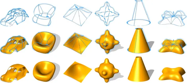
The method works well even for more challenging input data, such as the networks with large normal curvature variations and high valence curve intersections as illustrated in Figure 7. (simulated data)

Figure 7.Smooth surfaces reconstructed using our method.

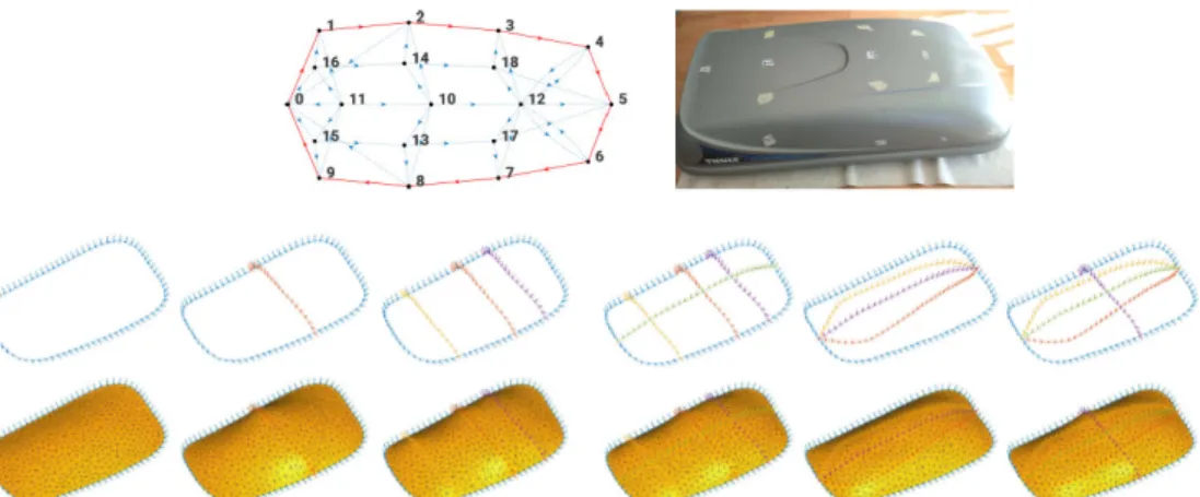
Finally, during acquisition, we often faced the question of what curves to acquire in order to minimize the error of reconstruction – different curve networks on the same surface often produce different results. Fig. 8 shows a roof box reconstructed with several different sets of curves, from the simplest one (only a single closed curve) to the richest one (larger mesh). The optimal choice of curves to be scanned is still to be investigated further on real use-cases, but goes beyond the scope of this paper.

(11)

Figure 8.Roof box acquired using the Morphorider and reconstructed with different sets of curves.

5. Conclusions

The Morphorider is an innovative device providing a new way to scan physical shapes. By its displacement on the surface, our approach provides first a robust curve network ready for surfacing, resolving challenges arising with real sensors (unknown positions: sensors measure local orientations of the surface – no absolute positions in the world space nor relative positions of two adjacent sensors are known; inconsistent data: intersecting curves often provide conflicting data, for instance two different normal for the same point in the world space; sensor noise: raw data from inertial sensors is noisy and needs to be pre-processed prior to reconstruction).

Our approach provides then a surface via a Laplacian-based surface reconstruction method from curve and normal input. After propagating the input normals smoothly over the surface and computing the corresponding mean curvature vectors, the normal constraints are integrated into the energy functional. Efficiency and robustness are achieved by using a linearized objective functional, such that the global optimization amounts to solve a sparse linear system of equations.

Most limitations of our method are device-related. The current Morphorider is a proof of concept and suffers from construction drawbacks. Its relatively big size limits the acquisition; it is often awkward to manipulate by the operator, and some regions with high curvature (in absolute value) could not have been scanned. Another problem is that the distance-measuring wheel is not aligned with the sensor unit – in practice this means that the covered distance relies mainly on magnetometers and thus the device cannot be used around ferromagnetic objects. The next generation of the prototype currently in development might help in resolving some of these problems and address specific application.

The Morphorider defines however a good tool for dynamical Structural Health Monitoring.

(12)

References

1. Sprynski N, David D, Lacolle B, Biard L. Curve Reconstruction via a Ribbon of Sensors. In: 14th IEEE Int. Conf. on Electronics, Circuits and Systems. 2007, p. 407–10.

2. Hoshi T, Shinoda H. 3D Shape Measuring Sheet Utilizing Gravitationa and Geomagnetic Fields. In: SICE Annual Conf. 2008, p. 915–20.

3. Saguin-Sprynski N, Jouanet L, Lacolle B, Biard L. Surfaces Reconstruction Via Inertial Sensors for Monitoring. In: 7th European Workshop on Structural Health Monitoring. 2014, p. 702–9.

4. N. Saguin-Sprynski, M. Carmona, L. Jouanet, and O. Delcroix. “New Generation of Flexible Risers Equipped with Motion Capture – Morphopipe System”. In: Proc. EWSHM – 8th European Workshop on Structural Health Monitoring. 2016. 5. J. L. Crassidis, F. L. Markley, and Y. Cheng. “Survey of nonlinear attitude

estimation methods”. In: J. Guid. Control Dyn. 30.1 (2007), pp. 12–28.

6. S. Bonnet et al. “Calibration methods for inertial and magnetic sensors”. In: Sensors and Actuators A: Physical 156.2 (2009), pp. 302–311.

7. M. P. do Carmo. Differential Geometry of Curves and Surfaces. Pearson, 1976. 8. J. L. Crassidis, F. L. Markley, and Y. Cheng. “Survey of nonlinear attitude

estimation methods”. In: J. Guid. Control Dyn. 30.1 (2007), pp. 12–28.

9. N. Boumal and P.-A. Absil. “A discrete regression method on manifolds and its application to data on SO(n)”. In: Proc. 18th IFAC WC. 2011, pp. 2284–2289. 10. N. Boumal. “Interpolation and Regression of Rotation Matrices”. In:

Geom.Sci.Inf. 2013, pp. 345–352.

11. W. Huang, P.-A. Absil, K. A. Gallivan, and P. Hand. ROPTLIB: An object-orient. C++ lib. for optim. On Riemannian manifolds. Tech. rep. FSU16-14.v2. 2016. 12. Zhuang Y, Zou M, Carr N, Ju T. A General and Efficient Method for Finding

Cycles in 3D Curve Networks. ACM Trans Graph (Proc SIGGRAPH Asia) 2013;32(6):180:1–180:10.

13. Shewchuk JR. Triangle: Engineering a 2D Quality Mesh Generator and Delaunay Triangulator. In: Applied computational geometry towards geometric engineering. Springer; 1996, p. 203–22.

14. Zou M, Ju T, Carr N. An Algorithm for Triangulating Multiple 3D Polygons. Computer Graphics Forum (SGP) 2013;32(5):157–66.

15. Botsch M, Sorkine O. On Linear Variational Surface Deformation Methods. IEEE Trans Vis Comput Graphics 2008;14(1):213–30.

16. Meyer M, Desbrun M, Schr¨oder P, Barr AH. Discrete Differential Geometry Operators for Triangulated 2-manifolds. In: Visualization and mathematics III. Springer; 2003, p. 35–57.

17. Botsch M, Kobbelt L, Pauly M, Alliez P, L´evy B. Polygon Mesh Processing. CRC press; 2010.

18. Sullivan J. Curvatures of Smooth and Discrete Surfaces. In: Bobenko A, Sullivan J, Schroder P, Ziegler G, editors. Discrete Differential Geometry; Oberwolfach Seminars Vol. 38. Birkhauser Basel; 2008, p. 175–88.