Elements of risk theory in finance and insurance

HAL Id: tel-01848801

https://tel.archives-ouvertes.fr/tel-01848801

HAL is a multi-disciplinary open access archive for the deposit and dissemination of sci-entific research documents, whether they are

pub-L’archive ouverte pluridisciplinaire HAL, est destinée au dépôt et à la diffusion de documents scientifiques de niveau recherche, publiés ou non,

Mina Mostoufi

To cite this version:

Mina Mostoufi. Elements of risk theory in finance and insurance. Sociology. Université Panthéon-Sorbonne - Paris I, 2015. English. �NNT : 2015PA010044�. �tel-01848801�

Ecole d’´

economie de Paris-PSE

THESE

pour obtenir le grade de Docteur

de l’Universit´e de Paris 1 Panth´eon-Sorbonne et de l’Ecole d’´economie de Paris-PSE

Discipline: Math´

ematiques Appliqu´

ees

pr´esent´ee par

Mina MOSTOUFI

le 17 D´ecembre 2015

ELEMENTS DE TH´

EORIE DU RISQUE EN

FINANCE ET ASSURANCE

Jury

M. Alain CHATEAUNEUF,

Directeur de th`ese

M. Phillip BICH,

Pr´esident du Jury

M. Robert KAST,

Rapporteur

Completion of this doctoral dissertation become possible with the support of several people. Throughout my Ph.D. career, their passionate and careful guidance helped me to perform a high quality research. I would like to express my sincere gratitude to all of them.

Foremost, I would like to express my deepest gratitude to my advisor Professor Alain Chateauneuf for his continuous supervision and valuable ideas and comments. During these three years, I have learned a lot from him, specially how to tackle new problems and how to develop techniques to solve them. Furthermore, I would like to thank Professor David Vyncke for sharing his experience and knowledge in the field of numerical methods. It was not possible for me to enter the challenging field of numerical methods without his help. Working with them was an honor for me, and they have always been patient and encouraging in challenging occasions of my PhD.

I would also like to thank my committee members, Dr. Robert KAST the Directeur de recherche au CNRS, Professor Andr´e LAPIED and Professor Phillipe BICH for serving as my thesis jury.

I am thankful to Paris School of Economics for providing financial resources for my re-search projects “Multivariate risk sharing and the derivation of individually rational Pareto optima” and “Comonotonic Monte Carlo and its applications in option pricing and quantifi-cation of risk”. Also I would like to acknowledge University of Paris 1 Panth´eon-Sorbonne for financing my research stay at Ghent University, Belgium as the International Mobility Scholarship.

In addition, I have been very privileged to get to know and to collaborate with my col-leagues and friends over the last three years at University of Paris 1 Panth´eon-Sorbonne and Ghent University. I learned a lot from them about life, research and how to approach challenging problems. I would like to thank them for they great spiritual supports and valuable comments.

Last but not the least, I would like to thank my family, specially Ghazal, Bardia and Reza. This dissertation would not have been possible without their warm love, continued patience, and endless support.

Cette th`ese traite de la th´eorie du risque en finance et en assurance. La mise en pra-tique du concept de comonotonie, la d´ependance du risque au sens fort, est d´ecrite pour identifier l’optimum de Pareto et les allocations individuellement rationnelles Pareto optim-tales, la tarification des options et la quantification des risques. De plus, il est d´emontr´e que l’aversion au risque monotone `a gauche, un raffinement pertinent de l’aversion forte au risque, caract´erise tout d´ecideur `a la Yaari, pour qui, l’assurance avec franchaise est optimale.

Le concept de comonotonie est introduit et discut´e dans le chapitre 1. Dans le cas de risques multiples, on adopte l’id´ee qu’une form naturelle pour les compagnies d’assurance de partager les risques est la Pareto optimalit´e risque par risque. De plus, l’optimum de Pareto et les allocations individuelles Pareto optimales sont caract´eris´ees.

Le chapitre 2 ´etudie l’application du concept de comonotonie dans la tarification des options et la quantification des risques. Une nouvelle variable de contrˆole de la m´ethode de Monte Carlo est introduite et appliqu´ee aux “basket options”, aux options asiatiques et `a la TVaR. Finalement dans le chapitre 3, l’aversion au risque au sens fort est raffin´e par l’introduction de l’aversion au risque monotone `a gauche qui caract´erise l’optimalit´e de l’assurance avec franchise dans le mod`ele de Yaari. De plus, il est montr´e que le calcul de la franchise s’effectue ais´ement.

This thesis deals with the risk theory in Finance and Insurance. Application of the Comono-tonicity concept, the strongest risk dependence, is described for identifying the Pareto op-tima and Individually Rational Pareto opop-tima allocations, option pricing and quantification of risk. Furthermore it is shown that the left monotone risk aversion, a meaningful refine-ment of strong risk aversion, characterizes Yaari’s decision makers for whom deductible insurance is optimal.

The concept of Comonotonicity is introduced and discussed in Chapter 1. In case of multiple risks, the idea that a natural way for insurance companies to optimally share risks is risk by risk Pareto-optimality is adopted. Moreover, the Pareto optimal and individually Pareto optimal allocations are characterized.

The Chapter 2 investigates the application of the Comonotonicity concept in option pricing and quantification of risk. A novel control variate Monte Carlo method is introduced and its application is explained for basket options, Asian options and TVaR.

Finally in Chapter 3 the strong risk aversion is refined by introducing the left-monotone risk aversion which characterizes the optimality of deductible insurance within the Yaari’s model. More importantly, it is shown that the computation of the deductible is tractable.

Introduction 13

0.1 General Introduction . . . 13

0.2 Chapter 1: Multivariate risk sharing and the derivation of individually rational Pareto optima . . . 13

0.3 Chapter 2: Comonotonic Monte Carlo and its applications in option pricing and quantification of risk . . . 14

0.4 Chapter 3: Optimality of deductible for Yaari’s model: a reappraisal . . 15

0.5 Summary of Results . . . 15

0.5.1 Multivariate risk sharing and the derivation of individually rational Pareto optima . . . 15

0.5.2 Comonotonic Monte Carlo and its applications in option pricing and quantification of risk . . . 18

0.5.3 Optimality of deductible for Yaari’s model: a reappraisal . . . 20

References 23 1 Multivariate risk sharing and the derivation of individually rational Pareto op-tima 26 1.1 Introduction . . . 26

1.2 Framework and Definitions . . . 28

1.3 Deriving all Pareto optima . . . 29

1.3.1 Pareto optima in the one-dimensional case . . . 29

1.3.2 Deriving all Pareto optima . . . 31

1.3.3 Two illustrating examples . . . 33

1.4 Deriving all individually rational Pareto optima . . . 35

1.4.1 Two illustrating examples . . . 36

1.4.2 Revisiting the insurance example of Landsberger and Meilijson (1994) 38 1.5 Conclusion . . . 41

2.1 Introduction . . . 44

2.2 Control Variate Monte Carlo Method . . . 45

2.3 Comonotonic Control Variate . . . 46

2.3.1 Comonotonic Upper Bound . . . 47

2.3.2 Additivity property . . . 48

2.4 Comonotonic Control Variate for Asian Options, Basket Options and Tail Value-at-Risk . . . 51 2.4.1 Asian Option . . . 51 2.4.2 Basket Option . . . 54 2.4.3 Tail Value-at-Risk . . . 60 2.5 Conclusion . . . 61 References 63 3 Optimality of deductible for Yaari’s model: a reappraisal. 65 3.1 Introduction . . . 65

3.2 Framework and Definitions . . . 66

3.2.1 Yaari’s Model . . . 67

3.2.2 Insurance contracts with Deductible structure . . . 67

3.3 Left monotone increase in risk . . . 68

3.3.1 Left monotone risk aversion . . . 69

3.4 Optimality of deductible characterizes left monotone risk averse Yaari’s de-cision maker . . . 70

3.5 Computing the optimal level of deductible for a left monotone Yaari decision maker . . . 73

3.6 Conclusion . . . 79

1.1 Probability of the states for example 1. . . 37

1.2 Initial probability of the states for example 2. . . 38

1.3 Converted to the uniform probability . . . 38

1.4 Insurance example of Landsberger and Meilijson (1994). . . 39

1.5 First extreme point . . . 40

1.6 Second extreme point . . . 40

2.1 Performance of the CoMC method in Asian option pricing . . . 53

2.2 G-7 index linked guaranteed investment certificate weightings . . . 57

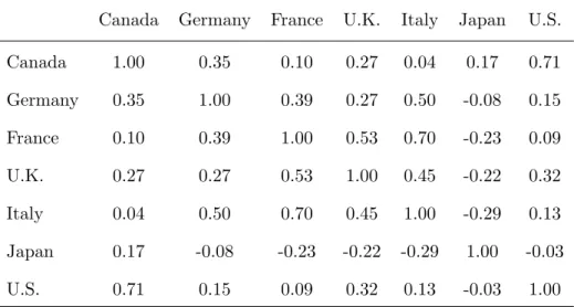
2.3 Correlation structure of the G-7 index . . . 57

2.4 Performance of the CoMC method in Basket option pricing . . . 58

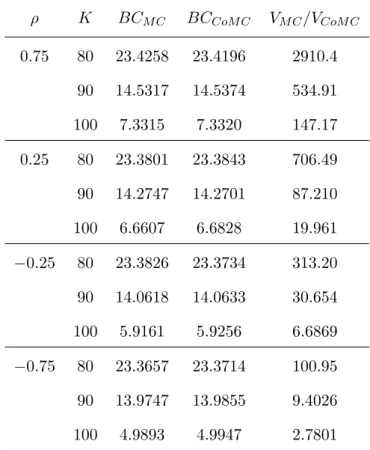
2.5 Influence of the correlation on the efficiency of CoMC . . . 59

2.6 Comparison of CoMC and geometric control variate . . . 60

0.1

General Introduction

This thesis deals with the risk theory in Finance and Insurance. Application of the Comono-toncity concept, the strongest risk dependence, is described for identifying the Pareto optima and Individually Rational Pareto optima allocations, option pricing and quantification of risk. Furthermore it is shown that the left monotone risk aversion, a meaningful refinement of strong risk aversion, characterizes Yaari’s decision makers for whom deductible insurance is optimal.

The concept of comonotonicty is introduced and discussed in Chapter 1. Moreover, the Pareto optimal and individually Pareto optimal allocations are characterized. Chapter 2 investigates the application of the Comonotonicity concept in option pricing and quantifica-tion of risk. In Chapter 3 the strong risk aversion is refined by introducing the left-monotone risk aversion which characterizes the optimality of deductible insurance within the Yaari’s model.

0.2

Chapter 1:

In a seminal paper, in case of strict strong risk averters assumed to be expected utility deci-sion makers, Borch (1962) characterized Pareto optimal risk sharing. The optimal sharing rule which depends on the specification of the utilities is based on a Mutuality Principle for risks which are fully diversifiable, furthermore Borch (1962) derived the precise conditions of the optimal allocations, which allow to compute the sharing of the Macroeconomic Risk (See for instance chapter 10 of Eeckhoudt et al. (2005) for more details).

It turns out that for expected utility decision makers with strictly increasing and strictly concave utility functions, Pareto optima are necessarily strictly comonotone i.e. strictly increasing functions of the aggregate endowments, but the converse is false.

As noticed by Landsberger and Meilijson (1994), the specific utilities of agents are hardly even known in practice, moreover let us add that the model which is used by an agent is

hardly even known as well. Consequently, Landsberger and Meilijson (1994) only assumed that agents are strictly strong risk averters in the sense of strict second order dominance. They obtained the nice result, that for such agents Pareto optimal allocations coincide exactly with the set of comonotone allocations i.e. the set of allocations which are non decreasing functions of the aggregate endowments. Landsberger and Meilijson (1994) gave a proof of the previous result and an algorithm allowing to reach at least one Pareto optimum, while they did not offer a method for computing all Pareto optima.

The main novelty provided by this work is to offer a complete characterization of Pareto optima, by extensively taking advantage of the polytope structure of these Pareto optima. Furthermore, it is shown that this strategy also allows to easily describe the entire convex set of individually rational Pareto optima—those for which every individual is better off when comparing with the initial situations—which clearly are those of practical interest in real life.

0.3

Chapter 2:

Monte Carlo (MC) simulation is a well known technique in different domains of mathe-matics such as mathematical finance, see Glasserman (2003); Benninga (2014). A typical application of the Monte Carlo method in finance is the estimation of the no-arbitrage price of a specific derivative security (e.g. a call option), which can be expressed as the expected value of its discounted payoff under the risk neutral measure. Another application of the Monte Carlo method in finance is estimating risk measures, such as Tail Value-at-Risk. The main shortcoming of the Monte Carlo method is its high computational cost. The standard error of the crude Monte Carlo estimate is of order O(√1

n) and thus, to double

the precision, one must run four times the number of simulations. Alternatively, strategies for reducing σ should be considered.

Several variance reduction techniques can be used in companion with the Monte Carlo method, such as antithetic variables, control variates and importance sampling. A detailed survey of these techniques is given in Ripley (1987). In chapter three we focus on the well-known control variate method for variance reduction which is based on the comonotonicty concept.

0.4

Chapter 3:

In the framework of EU model, Arrow (1965) proved that for a given premium, the optimal insurance contract for a EU risk averse decision maker is a contract with deductible. Gollier and Schlesinger (1996) obtained a nice generalization of this result by proving that this result holds also under strong aversion, whatever be the decision maker’s decision model under risk.

Vergnaud (1997) refined this result by proving that for any left monotone risk averse decision maker (not necessarily strongly risk averse), whatever be the decision model under risk, the optimal contract for a given premium is a deductible policy.

This last result is important since strong risk aversion is disputable in some situations, while Jewitt (1989)’s refinement i.e. left monotone risk aversion appears to be better adapted to insurance. This adds further justification to RDEU (rank-dependent expected utility) models and in particular to Yaari (1987)’s model that allow the decision maker to be left monotone risk averse without being strongly risk averse, which is impossible in the EU model, see Chateauneuf et al. (2004). In this chapter the optimality of deductible in the framework of Yaari’s model is revisited.

0.5

Summary of Results

0.5.1 Multivariate risk sharing and the derivation of individually rational Pareto optima

In case of multiple risks, we did adopt the idea that a natural way for insurance companies to optimally share risks is risk by risk Pareto-optimality. Our framework is based upon the well-known results in the one dimensional case characterizing Pareto-optimality as comono-tonicity in case of strong risk aversion. A simple computable method is offered for deriving all Pareto-optima and deriving all Individually Rational Pareto-optima.

Definitions and Preliminary Results

The definitions, lemmata and theorems which exploited to obtain the results of chapter 1 are given as follows.

Definition 0.5.1. X = (X1, . . . , Xi, . . . , Xn) ∈ (Rm)p×n is Pareto optimal if ∀k ∈ �1, p�

(X₁k, . . . , X_ik, . . . , X_nk) is Pareto optimal in the usual sense for the univariate case with

re-spect to the second order stochastic dominance i.e. for k given, (Xk

feasible allocation:

Xk

i ∈ Rm+ ∀i,

�n

i=1Xik = wk and there does not exist Y = (Y1k, . . . , Yik, . . . , Ynk),

Y_ik ∈ Rm + ∀i,

�n

i=1Yik = wk, such that Yik�SSDXik ∀i and Yik0�SSDX

k

i0 for some i0.

Definition 0.5.2. X = (X1, . . . , Xi, . . . , Xn)∈ (Rm)p×n is an individually rational Pareto

optimum if X is Pareto optimal and individually rational i.e. ∀i, k Xk

i�SSDwki.

Definition 0.5.3. An allocation X = (X1, . . . , Xi, . . . , Xn) is comonotone if,

∀(i, i�)∈ �1, n�2 (Xi(s)− Xi(t))�X_i�(s)− X

i� (t)� ≥ 0 ∀ (s, t) ∈ S2.

Theorem 0.5.4. The set of Pareto optimal allocations coincide with the set of comonotone allocations.

Lemma 0.5.5. Any Pareto optimal allocation is comonotone.

Lemma 0.5.6. Any comonotone allocation is Pareto optimal.

Lemma 0.5.7. Let w(sj) = wj. Then after possibly relabeling, if needed, the indices in

such a way that w1≤ . . . ≤ wj ≤ . . . ≤ wm, one gets: If (Xi)i=1,...,n is a feasible allocation,

then the two following properties are equivalent;

(i) (Xi)i=1,...,n is comonotone.

(ii) Xi(1)≤ . . . ≤ Xi(j)≤ . . . ≤ Xi(m) ∀i = 1, . . . , n.

Remark 0.5.8. It is worth noticing that building upon Lemma 0.5.7, Theorem 0.5.4 can be restated, in accordance with some economic terminology (For instance see Eeckhoudt et al. (2005)), see Theorem 0.5.9 below.

Theorem 0.5.9. For an allocation X = (X1, . . . , Xi, . . . , Xn) ∈ Rm×n the two following

assertions are equivalent:

(i) X is Pareto optimal

2. Mutuality Principle:

∀s, t ∈ S w(s) = w(t) =⇒ Xi(s) = Xi(t) ∀i = 1, ..., n

3. Weak comonotonicity:

∀s, t ∈ S w(s) < w(t) =⇒ Xi(s)≤ Xi(t) ∀i = 1, ..., n

Remark 0.5.10. Let us recall again that for strict strong risk averters who are EU (expected utility decision makers) Pareto optima satisfy (ii).1, (ii).2 but (ii).3 should be replaced by strict comonotonicity (see Borch (1962) or also Eeckhoudt et al. (2005)) i.e. ∀s, t ∈ S w(s) < w(t)=_⇒Xi(s) < Xi(t) ∀i = 1, ..., n.

Theorem 0.5.11. The set of Pareto optima is a polytope, hence it is the convex hull of its

finitely many extreme points.

Lemma 0.5.12. Any individually rational Pareto optimum (IRPO) Xiis such that E(Xi) =

E(wi).

Lemma 0.5.13. The set PIR of individually rational Pareto optima is nonempty.

Remark 0.5.14. Note that in the present paper, we intend to systematically derive all IRPO’s at least for rational probabilities (which apparently in “real life” is not a severe limitation). Our result contrasts from the algorithms which can be found in the literature. Actually these algorithms propose a method to obtain only one IRPO (see e.g. Landsberger and Meilijson (1994) or Ludkovski and R¨uschendorf (2008)), but not all IRPO’s.

Remark 0.5.15. Note that even for a finite state space S , it is not easy to express the individually rational conditions Xi�SSDwi, i = 1, . . . , n. Actually Xi�SSDwi is equivalent

to � p 0 F_X−1_i(t)dt≥ � p 0 F_w−1_i (t)dt ∀p ∈ (0, 1) (0.1)

with equality if p=1, as noticed in Lemma 0.5.12, but even if (0.1) has to be checked only for a finite number p� ∈ (0, 1), in practice finding which p� must be chosen is a delicate

task. In contrast, if each pj is a rational probability, let us say of the type pj = k_qj where

kj, q∈ N∗+, it is immediate that Xi�SSDwi iff

� k q 0 F_X−1_i(t)dt≥ � k q 0 F_w−1_i (t)dt ∀k ∈ �1, q�.

Theorem 0.5.16. The set PIR of individually rational Pareto optima is a polytope, hence

the convex hull of its finitely many extreme points.

Theorem 0.5.17. Assume that the initial endowment of agent i is wi ∈ Rm and define the

IRP O’s as the allocations X = (X1, . . . , Xi, . . . , Xn)∈ Rm×n such that�_iXi =�_iwi (:=

w) and Xi�SSDwi ∀i, then the set PIR is the polytope of the feasible allocations which are

comonotone and satisfy the individually rational constraints.

0.5.2 Comonotonic Monte Carlo and its applications in option pricing and quantification of risk

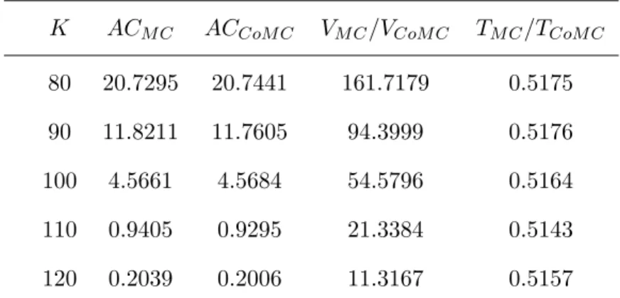
A novel control variate Monte Carlo method (CoMC) is presented based on the concept of comonotonicity. This method is explained for basket options, Asian options and TVaR. We evaluated the performance of the method in realistic cases by illustrative numerical examples. The realistic benchmark examples show that the precision of estimating the price of Asian and Basket options is drastically increased by employing the CoMC method while the computation time is not increased considerably compared to the crude Monte Carlo method.

Definitions and Preliminary Results

The definitions, lemmata and theorems which exploited to obtain the results of chapter 2 are given as follows.

Definition 0.5.18. A random vector X = (X1, ..., Xn) is comonotonic if and only if it has

a comonotonic copula i.e. for all x = (x1, ..., xn), we have

FX(x) = min {FX1(x1), FX2(x2), ..., FXn(xn)} . (0.2)

Proposition 0.5.19. If X has a comonotonic copula then for U _{∼ Uniform(0, 1), we have}

X= (Fd _X−1₁(U ), (F_X−1₂(U ), ..., (F_X−1_n(U )). (0.3) Proposition 0.5.20. The quantile function FS−1c of a sum Sc of comonotonic random

vari-ables with distribution functions FX1, ..., FXn is additive

FS−1c (p) = n � i=1 F_X−1 i(p), 0 < p < 1. (0.4)

Definition 0.5.21. The distorted expectation of a random variable X is defined by ρg[X] = � 0 −∞ �g( ¯FX(x))− 1� dx + � ∞ 0 g( ¯FX(x))dx, (0.5)

where ¯FX(x) = 1− FX(x) denotes the tail function of FX(x) and the function g(.) is a

so-called distortion function, i.e. a non-decreasing function g : [0, 1] _{−→ [0, 1] such that}

g(0) = 0 and g(1) = 1.

Proposition 0.5.22. The distortion risk measure for a sum of comonotonic variables is additive i.e. for any distortion function g and all random variables Xi we have

ρg[Sc] = n

�

i=1

ρg[Xi]. (0.6)

Corollary 0.5.23. The Tail Value-at-Risk, T V aRX(p), at level p∈ (0, 1) given by

T V aRX(p) = 1

1− p � 1

p

F_X−1(q)dq (0.7)

is a distortion risk measure with distortion function

g(x) = min � x 1_{− p}, 1 � , 0≤ x ≤ 1,

hence it is additive for comonotonic random variables.

Corollary 0.5.24. The ESF (Expected shortfall) can be written as a linear combination of distortion risk measures given by

T V aRX(p) = FX−1(p) +

1

1_{− p}ESFX(p),

see Dhaene et al. (2006), thus it follows

ESFSc(p) = (1− p)(T V aRSc(p)− F_S−1_c (p)) = (1_{− p)} � _n � i=1 T V aRXi(p)− n � i=1 F−1 Xi(p) � = n � i=1 ESFXi(p), 0 < p < 1.

Corollary 0.5.25. By choosing p = FSc(K) in Corollary 0.5.24, it follows that the stop-loss

premium E[(Sc−K)+] of a sum Sc of comonotonic random variables with strictly increasing

distribution functions FX1, ..., FXn can be written as

E[(Sc_{− K)}+] = n

�

i=1

[(Xi− F_X−1_i(FSc(K)))₊], ∀K ∈ R. (0.8)

0.5.3 Optimality of deductible for Yaari’s model: a reappraisal

The main purpose of this chapter is to show that, within the Yaari’s model, left-monotone risk aversion does characterize the optimality of deductible insurance. Moreover, it is shown that for such left-monotone Yaari’s risk averters, the computation of the deductible is very tractable.

Definitions and Preliminary Results

The definitions, Lemmata and theorems which exploited to obtain the results of chapter 3 are given as follows.

Definition 0.5.26. For random variables X and Y with the same mean, Y is a left

mono-tone increase in risk of X if �F_Y−1(p)

−∞ FY(p)≥

�F_X−1(p)

−∞ FX(p), ∀p ∈ [0, 1]. Let us recall that

for any distribution F i.e. any mapping F : R−→ R non-decreasing, right-continuous such

that lim_t→−∞F (t) = 0, lim_t→+∞F (t) = 1, F−1 _{: [0, 1] −→ R is defined ∀p ∈ [0, 1] by}

F−1_{(p) = inf�t ∈ ¯R, F (t) ≥ p�. Note that F}−1_{(0) =−∞.}

Lemma 0.5.27. For every pair (X, Y ) of discrete random variables with E(X) = E(Y ) such that Y is a left monotone increase in risk of X, Y can be reached from X by a finite sequence of transfers as in (3.3).

Definition 0.5.28. Distribution G is a left-monotone simple spread of F if

1. E(G) = E(F ) 2. _{∃ p}0 ∈ (0, 1) such that: p_{≤ p}0 =⇒ (2.1) G−1(p)≤ F−1(p) (2.2) d(p) = F−1_{(p)− G}−1_{(p) is non-increasing on (0, p} 0] p > p0 =⇒ (2.3) G−1(p)≥ F−1(p).

Lemma 0.5.29. If G is a left-monotone simple spread of F then F is left-monotone less risky than G.

Lemma 0.5.30. Any Yaari decision maker is a left monotone increase in risk if and only if the probability transformation function is star shaped1at 1 i.e. 1−f(p)_1−p is an increasing function of p on [0, 1).

Theorem 0.5.31. Any Yaari’s decision maker who has preference for deductibles with any given premium is a left-monotone risk averse.

Lemma 0.5.32. Any decision maker who exhibits preference for deductible will prefer

L_{(X) = (x1, p1; x2, p2; x3, p3; x4, p4) to L (Y ) = (x1−�p3, p1; x2, p2; x3+ �p1, p3; x4, p4),}

[Recall that through the definitions of the “L ”, one has pi ≥ 0, �4_i=1pi= 1 and x1 < x2 <

x3< x4 and x1− �p3< x2 < x3+ �p1 < x4].

Remark 0.5.33. Note that if we had required that indemnities should satisfy the Moral Hazard requirement i.e. that what remains to be paid by the decision maker namely D_−I(D) should increase with the amount of the damage our Lemma 0.5.32 would remain valid. Actually: d4− I(d4) = 0 < d3− I(d3) = x4− x3− �p1 < d2− I(d2) = x4− x2 < d1− I(d1) =

x4− x1+ �p3.

Remark 0.5.34. The proof of Theorem 0.5.31 shows that it is enough that a Yaari’s de-cision maker has preference for deductible only in case of finite discrete random losses, in order to be a left-monotone risk averter.

Theorem 0.5.35. (Vergnaud (1997)) Any left-monotone risk-averse decision maker has preference for deductible.

Theorem 0.5.36. A strict left monotone risk averse Yaari decision maker will purchase full insurance if

(1 + m)(1_{− F (0)) − (1 − f(F (0))) < 0} (0.9)

1_{A function f ∈ F is star-shaped at m, if:} f(m)−f (p)

m−p

Otherwise, ¯d is an optimal level of deductible if and only if it satisfies

(1 + m)(1_{− F ( ¯}d₋))_{− (1 − f(F ( ¯}d₋)))_{≥ 0 ≥ (1 + m)(1 − F ( ¯}d))_{− (1 − f(F ( ¯}d))). (0.10) Remark 0.5.37. If F is continuous, indeed the inequality 0.10 in theorem 0.5.36 reduces to the following simple equation:

(1 + m)(1− F ( ¯d))− (1 − f(F ( ¯d))) = 0

Lemma 0.5.38. Let u : [a, b]_{−→ R be continuous and such that u}�₊(·) exists on (a, b) with u�₊(x)≤ 0 ∀x ∈ (a, b) then u is non-increasing on [a, b] .

Lemma 0.5.39. Let u : [a, b]_{−→ R be continuous and such that u}�₊(·) exists and strictly

Albrecher, H., Dhaene, J., Goovaerts, M., Schoutens, W., 2005. Static hedging of Asian options under L´evy models. The Journal of Derivatives 12, 63–72.

Arrow, K.J., 1965. Aspects of the theory of risk-bearing. Yrj¨o Jahnssonin S¨a¨ati¨o. Benninga, S., 2014. Financial modeling. MIT press.

Borch, K., 1962. Equilibrium in a reinsurance market. Econometrica 30, 424–444.

Carlier, G., Dana, R.A., Galichon, A., 2012. Pareto efficiency for the concave order and multivariate comonotonicity. Journal of Economic Theory 147, 207–229.

Chateauneuf, A., Cohen, M., Meilijson, I., 2004. Four notions of mean-preserving increase in risk, risk attitudes and applications to the rank-dependent expected utility model. Journal of Mathematical Economics 40, 547–571.

Chateauneuf, A., Cohen, M., Meilijson, I., et al., 1997. New Tools to Better Model Behavior Under Risk and UNcertainty: An Oevrview. Technical Report. Universit´e de Paris1 Panth´eon-Sorbonne (Paris 1).

Chateauneuf, A., Dana, R.A., Tallon, J.M., 2000. Optimal risk-sharing rules and equilibria with choquet-expected-utility. Journal of Mathematical Economics 34, 191–214.

Deelstra, G., Dhaene, J., Vanmaele, M., 2011. An overview of comonotonicity and its applications in finance and insurance, in: Advanced mathematical methods for finance. Springer, pp. 155–179.

Denuit, M., Dhaene, J., 2012. Convex order and comonotonic conditional mean risk sharing. Insurance: Mathematics and Economics 51, 265 – 270.

Dhaene, J., Denuit, M., Goovaerts, M.J., Kaas, R., Vyncke, D., 2002. The concept of comonotonicity in actuarial science and finance: theory. Insurance: Mathematics and Economics 31, 3–33.

Dhaene, J., Linders, D., Schoutens, W., Vyncke, D., 2014. A multivariate dependence measure for aggregating risks. Journal of Computational and Applied Mathematics 263, 78–87.

Dhaene, J., Vanduffel, S., Goovaerts, M., Kaas, R., Tang, Q., Vyncke, D., 2006. Risk measures and comonotonicity: a review. Stochastic models 22, 573–606.

Doherty, N.A., Eeckhoudt, L., 1995. Optimal insurance without expected utility: The dual theory and the linearity of insurance contracts. Journal of Risk and Uncertainty 10, 157–179.

Eeckhoudt, L., Gollier, C., Schlesinger, H., 2005. Economic and financial decisions under risk. Princeton University Press.

Florenzano, M., Le Van, C., Gourdel, P., 2001. Finite dimensional convexity and optimiza-tion. Springer New York.

Glasserman, P., 2003. Monte Carlo methods in financial engineering. volume 53. Springer Science & Business Media.

Gollier, C., Schlesinger, H., 1996. Arrow’s theorem on the optimality of deductibles: a stochastic dominance approach. Economic Theory 7, 359–363.

Jewitt, I., 1989. Choosing between risky prospects: the characterization of comparative statics results, and location independent risk. Management Science 35, 60–70.

Kaas, R., Dhaene, J., Goovaerts, M.J., 2000. Upper and lower bounds for sums of random variables. Insurance: Mathematics and Economics 27, 151–168.

Kemna, A.G., Vorst, A., 1990. A pricing method for options based on average asset values. Journal of Banking & Finance 14, 113–129.

Landsberger, M., Meilijson, I., 1994a. Co-monotone allocations, bickel-lehmann dispersion and the arrow-pratt measure of risk aversion. Annals of Operations Research 52, 97–106. Landsberger, M., Meilijson, I., 1994b. The generating process and an extension of jewitt’s

location independent risk concept. Management Science 40, 662–669.

Liu, X., Mamon, R., Gao, H., 2013. A comonotonicity-based valuation method for guaran-teed annuity options. Journal of Computational and Applied Mathematics 250, 58–69. Ludkovski, M., R¨uschendorf, L., 2008. On comonotonicity of pareto optimal risk sharing.

Madan, D.B., Carr, P.P., Chang, E.C., 1998. The variance gamma process and option pricing. European finance review 2, 79–105.

MATLAB, 2010. version 7.10.0 (R2010a). The MathWorks Inc., Natick, Massachusetts. Milevsky, M.A., Posner, S.E., 1998a. A closed-form approximation for valuing basket

op-tions. The Journal of Derivatives 5, 54–61.

Milevsky, M.A., Posner, S.E., 1998b. Erratum: A closed-form approximation for valuing basket options. The Journal of Derivatives 6, 83.

Quiggin, J., 1982. A theory of anticipated utility. Journal of Economic Behavior & Orga-nization 3, 323–343.

Ripley, B.D., 1987. Stochastic simulation. Wiley & Sons, New York.

Sandstr¨om, A., 2010. Handbook of solvency for actuaries and risk managers: theory and practice. CRC Press.

Simon, S., Goovaerts, M., Dhaene, J., 2000. An easy computable upper bound for the price of an arithmetic asian option. Insurance: Mathematics and Economics 26, 175–183. Tsuzuki, Y., 2013. On optimal super-hedging and sub-hedging strategies. International

Journal of Theoretical and Applied Finance 16.

Vergnaud, J.C., 1997. Analysis of risk in a non-expected utility framework and application to the optimality of the deductible. Revue Finance 18, p155–167.

Vyncke, D., Goovaerts, M., Dhaene, J., 2001. Convex upper and lower bounds for present value functions. Applied Stochastic Models in Business and Industry 17, 149–164. Wang, S., 1996. Premium calculation by transforming the layer premium density. ASTIN

Bulletin 26, 71–92.

Yaari, M.E., 1987. The dual theory of choice under risk. Econometrica: Journal of the Econometric Society , 95–115.

Multivariate risk sharing and the

deriva-tion of individually raderiva-tional Pareto optima

1

Alain Chateauneuf, Mina Mostoufi, David Vyncke

Abstract

Considering that a natural way of sharing risks in insurance companies is to require risk by risk Pareto optimality, we offer in case of strong risk aversion, a simple com-putable method for deriving all Pareto optima. More importantly all Individually Rational Pareto optima can be computed according to our method.

Keywords : Multivariate risk sharing, Comonotonicity, Individually rational Pareto optima.

JEL classification: D70, D81.

1.1

Introduction

In a seminal paper, in case of strict strong risk averters assumed to be expected utility decision makers, Borch (1962) characterized Pareto optimal risk sharing. The optimal sharing rule which depends on the specification of the utilities is based on a Mutuality Principle for risks which are fully diversifiable, furthermore Borch (1962) derived the precise conditions of the optimal allocations, which allow to compute the

1_{This paper is published in the Journal of Mathematical Social Sciences, Vol. 74, Pages 73 − 78,}

sharing of the Macroeconomic Risk (See for instance chapter 10 of Eeckhoudt et al. (2005) for more details).

It turns out that for expected utility decision makers with strictly increasing and strictly concave utility functions, Pareto optima are necessarily strictly comonotone i.e. strictly increasing functions of the aggregate endowments, but the converse is false.

As noticed by Landsberger and Meilijson (1994), the specific utilities of agents are hardly even known in practice, moreover let us add that the model which is used by an agent is hardly even known as well. Consequently, Landsberger and Meilijson (1994) only assumed that agents are strictly strong risk averters in the sense of strict second order dominance.

They obtained the nice result, that for such agents Pareto optimal allocations coincide exactly with the set of comonotone allocations i.e. the set of allocations which are non decreasing functions of the aggregate endowments. Landsberger and Meilijson (1994) gave a proof of the previous result and an algorithm allowing to reach at least one Pareto optimum, while they did not offer a method for computing all Pareto optima. The main novelty provided by this work is to offer a complete characterization of Pareto optima, by extensively taking advantage of the polytope structure of these Pareto optima. Furthermore, it is shown that this strategy also allows to easily describe the entire convex set of individually rational Pareto optima—those for which every individual is better off when comparing with the initial situations—which clearly are those of practical interest in real life.

This is performed under the mild assumption that the underlying probability informa-tion (we just consider a finite set of states of nature) consists of rainforma-tional probabilities. This is not a too restrictive assumption since any probabilistic information can indeed be approximated as far as needed by such rational probabilities.

As a dividend in case of multidimensional risk sharing if multidimensional risk aver-sion, is defined as strict strong risk aversion component by component, which would prove to be meaningful in case of extreme caution, then multidimensional Pareto optima, reduce to one dimensional Pareto optima component by component and therefore can be easily computed through our proposed method.

Indeed, in this way we avoid using a generalized comonotone dominance principle, which is in accordance with the multidimensional second order stochastic dominance, as this is developed by Carlier et al. (2012) in order to obtain other types of Pareto optima, which apparently might be difficult to derive analytically.

The paper is organized as follows. Section 1.2 presents the general framework of multidimensional risk sharing, recalls some definitions and shows how the problem reduces to one dimensional Pareto optima. Section 1.3 deals with the characterization of Pareto optimal risk sharing, while section 1.4 offers a description of individually rational Pareto optima.

As an application, we derive all individually rational Pareto optima linked with the insurance problem examined by Landsberger and Meilijson (1994). This example illustrates how IRPO’s (individually Rational Pareto optimal risk sharings) allow reducing risks which are not initially covered by the insurance policy. Finally, section 1.5 discusses the obtained results and concludes the paper.

1.2

Framework and Definitions

Consider, for the purpose of illustration, n insurance companies, i = 1, . . . , n, each holds at date zero, p portfolios of insurance of type k = 1, . . . , p leading at date one to future stochastic wealth Xk

i :�S, 2S, P� → R+ , where S = (s1, . . . , sj, . . . , sm) is

the finite space of the sets of nature, and P the probability on 2S _{is given and satisfies}

P (sj) = pj > 0 ∀j.

Let wi = (w1i, . . . , wik, . . . , w p

i) be the initial endowment of insurance i with respect to

each portfolio of type k, i.e. each future wealth in each state with respect to premia and reimbursements related to type k. Denote wk ₌

n

�

i=1

w_ik.

By definition, X is a feasible allocation if X = (X1, . . . , Xi, . . . , Xn) with Xi ∈

�Rm + �p ∀i = 1, . . . , n and n � i=1 Xk i = wk ∀k ∈ �1, p�.

Let us now recall that if X and Y are bounded real random variables, X dominates Y by the second order stochastic dominance i.e. X is considered as less risky than Y denoted by X_�SSDY if

�p

0 FX−1(t)dt≥

�p

0 FY−1(t)dt ∀p ∈ �0, 1� where F−1 is the usual

quantile function.

Moreover X_�SSDY i.e. X strictly dominates Y for the second order stochastic

dom-inance if furthermore �p0

0 FX−1(t)dt >

�p0

0 FY−1(t)dt for some p0 ∈ (0, 1].

We assume that each agent i has preferences _�i associated with the component by

component second order stochastic dominance that is for Xi = (Xi1, . . . , Xik, . . . , X p i)∈ �Rm + �p and Yi = (Yi1, . . . , Yik, . . . , Y p i )∈�Rm+ �p then if Xk i�SSDYik ∀k ∈ �1, p� one has

that Xk0

i �SSDYik0 then Xi is strictly preferred to Yi i.e. Xi�iYi.

From the above assumptions it turns out that:

Definition 1.2.1. X = (X1, . . . , Xi, . . . , Xn) ∈ (Rm)p×n is Pareto optimal if ∀k ∈

�1, p� (Xk

1, . . . , Xik, . . . , Xnk) is Pareto optimal in the usual sense for the

univari-ate case with respect to the second order stochastic dominance i.e. for k given, (Xk

1, . . . , Xik, . . . , Xnk) is a feasible allocation:

Xk

i ∈ Rm+ ∀i,

�n

i=1Xik = wk and there does not exist Y = (Y1k, . . . , Yik, . . . , Ynk),

Yk

i ∈ Rm+ ∀i,

�n

i=1Yik = wk, such that Yik�SSDXik ∀i and Yik0�SSDX

k

i0 for some i0.

Definition 1.2.2. X = (X1, . . . , Xi, . . . , Xn) ∈ (Rm)p×n is an individually rational

Pareto optimum if X is Pareto optimal and individually rational i.e. _{∀i, k X}k

i�SSDwik.

1.3

Deriving all Pareto optima

From Definition 1.2.1 it turns out that the p-dimensional case reduces to p one di-mensional situations. So we just have to deal with the following situation:

X = (X1, . . . , Xi, . . . , Xn) Xi :�S, 2S, P� → R+, w∈ Rm+ given.

In subsection 2.3.1 for the sake of completeness we just propose what we hope to be a very simple, direct and complete proof of the well-known characterization of Pareto optimal allocations in terms of comonotonicity.

1.3.1 Pareto optima in the one-dimensional case

Definition 1.3.1. An allocation X = (X1, . . . , Xi, . . . , Xn) is comonotone if,

∀�i, i�

� ∈ �1, n�2

(Xi(s)− Xi(t)) (Xi�(s)− Xi� (t))≥ 0 ∀ (s, t) ∈ S2.

We intend to retrieve, in a simple way, the well-known following theorem, which is implicit in Landsberger and Meilijson, see Landsberger and Meilijson (1994).

Theorem 1.3.2. The set of Pareto optimal allocations coincide with the set of comono-tone allocations.

The proof will result from the following two lemmas.

Lemma 1.3.3. Any Pareto optimal allocation is comonotone.

Proof: We just sketch the proof given in Chateauneuf et al. (2000). It is enough to show that any non-comonotone allocation X = (X1, . . . , Xi, . . . , Xn) can be improved

to a new allocation X� = �X�

1, . . . , X

�

i, . . . , X

�

n� which is mutually beneficial for all

agents and strictly beneficial for at least one.

Let us assume, without loss of generality, that comonotonicity is not satisfied for X1

, X2 and for s1 , s2. Let X1(s1) = x1, X1(s2) = x2, X2(s1) = y1, X2(s2) = y2 and

assume without loss of generality that x1 + y1 ≤ x2+ y2, x1 > x2 and y1 < y2.

Let us modify (x1, x2) to�x � 1, x � 2� and (y1, y2) to�y � 1, y � 2� where x � 1 = x � 2 = p1x1+ p2x2 p1+ p2 , y₁� = x1+ y1− x � 1 and y � 2 = x2+ y2− x � 2.

Therefore X = (X1, . . . , Xi, . . . , Xn) has been modified to, X

� = (X₁�, X₂�, X₃�, . . . , Xn � ) where Xi � = Xi ∀i = 3, . . . , n.

It is then straightforward to see that we obtain a new allocation X� and that Xi

�

is strictly less risky than Xi for i = 1, 2 since E(u(Xi

�

)) > E (u (Xi)) for any strictly

concave utility function u, which completes the proof. ✷ Lemma 1.3.4. Any comonotone allocation is Pareto optimal.

Proof: Let X = (X1, . . . , Xi, . . . , Xn) be a comonotone allocation. We just intend to

show that it is impossible that a feasible allocation Y = (Y1, . . . , Yi, . . . , Yn) strictly

dominates X. Without loss of generality, we assume that Y1�SSDX1 i.e. there exists

p0 ∈ (0, 1] such that: � p0 0 F−1 Y1 (t)dt > � p0 0 F−1 X1(t)dt and, � p 0 F_Y−1₁ (t)dt ≥ � p 0 F_X−1₁(t)dt and ∀p ∈ [0, 1]. Moreover �p 0 FY−1i (t)dt ≥ �p 0 FX−1i(t)dt ∀i ∀p ∈ [0, 1]. Hence we get, n � i=1 � p0 0 F−1 Yi (t)dt > n � i=1 � p0 0 F−1 Xi(t)dt (1.1)

Let us now show that,

n � i=1 � p0 0 F−1 Yi (t)dt≤ � p0 0 F_�−1_n i=1Yi(t)dt (1.2)

Recall that TVAR is sub-additive see Denuit and Dhaene (2012), i.e. for any random variable Z, TVAR(Z,p) = _1−p1 �1

random variables T and Z one gets:

TVAR(Z+T,p)≤ TVAR(Z,p)+TVAR(T,p). From E(Z) = �1

0 FZ−1(t))dt, E(T ) =

�1

0 FT−1(t))dt and indeed E(Z + T ) = E(Z) +

E(T ) it is then straightforward to obtain: � p0 0 F−1 Z+T(t)dt ≥ � p0 0 F−1 Z (t)dt + � p0 0 F−1 T (t)dt.

And therefore by induction one gets (1.2). Combining (1.1) and (1.2) we obtain:

n � i=1 � p0 0 F−1 Xi(t)dt < � p0 0 F_�−1 n i=1Yi(t)dt (1.3) But �n i=1Xi = w = �n i=1Yi hence Fw−1 = F�−1n i=1Xi = F −1 �n

i=1Yi, moreover since X

is comonotone F_�−1

n

i=1Xi =

�n

i=1FX−1i a.e. (almost everywhere) thus (1.3) implies:

�p0

0 Fw−1(t)dt <

�p0

0 Fw−1(t)dt a contradiction, which completes the proof of lemma

1.3.4 and henceforth of Theorem 1.3.2. ✷

1.3.2 Deriving all Pareto optima

We intend now to show that the set of Pareto optima is a polytope. Therefore by implementing the vertex identification algorithm as can be found in MATLAB (2010), one can easily obtain all Pareto optima. Let us start by a preliminary lemma. Lemma 1.3.5. Let w(sj) = wj. Then after possibly relabeling, if needed, the indices

in such a way that w1 ≤ . . . ≤ wj ≤ . . . ≤ wm, one gets: If (Xi)i=1,...,n is a feasible

allocation, then the two following properties are equivalent; (i) (Xi)i=1,...,n is comonotone.

(ii) Xi(1)≤ . . . ≤ Xi(j)≤ . . . ≤ Xi(m) ∀i = 1, . . . , n.

Proof:

(i)=⇒(ii): Let wj ≤ wj+1 and assume there exists i0 such that Xi0(j) > Xi0(j + 1).

Since (Xi)i=1,...,n is comonotone, we have Xi(j)≥ Xi(j + 1)∀i �= i0. Summing up both

sides of the inequality over i = 1, . . . , n gives �n

i=1Xi(j) >

�n

i=1Xi(j + 1).

Since (Xi)i=1,...,n is a feasible allocation, the following relation wj > wj+1 is obtained,

(ii)=_{⇒(i): Take j �= j}�. From (ii) we have:

Xi(1) ≤ . . . ≤ Xi(j) ≤ . . . ≤ Xi(m) ∀i = 1, . . . , n, therefore it is immediate that

∀i �= i� (Xi(j)− Xi(j

�

))(X_i�(j)− X

i�(j

�

))_{≥ 0, which means that the X}i ’s are pairwise

comonotone. ✷

Remark 1.3.6. It is worth noticing that building upon Lemma 1.3.5, Theorem 1.3.2 can be restated, in accordance with some economic terminology (For instance see Eeckhoudt et al. (2005)), see Theorem 1.3.7 below.

Theorem 1.3.7. For an allocation X = (X1, . . . , Xi, . . . , Xn) ∈ Rm×n the two

fol-lowing assertions are equivalent: (i) X is Pareto optimal

(ii) 1. X is feasible 2. Mutuality Principle: ∀s, t ∈ S w(s) = w(t) =_{⇒ X}i(s) = Xi(t) ∀i = 1, ..., n 3. Weak comonotonicity: ∀s, t ∈ S w(s) < w(t) =_{⇒ X}i(s)≤ Xi(t) ∀i = 1, ..., n Proof:

(i)=⇒(ii) is immediate since by definition, Pareto optima are feasible. It can be concluded from Theorem 1.3.2 that X is comonotone, therefore from lemma 1.3.5 we have:

w(s)_{≤ w(t) and w(t) ≤ w(s) implies X}i(s) = Xi(t) ∀i.

Also we have, w(s) < w(t)=_⇒Xi(s)≤ Xi(t) ∀i.

(ii)=⇒(i) Let i, j ∈ {1, ..., n} and s, t ∈ S indeed if Xi(s) = Xi(t) then

(Xi(s)− Xi(t)) (Xj(s)− Xj(t)) ≥ 0, and by symmetry if Xi(s) < Xi(t) then

w(s) < w(t), therefore it can be concluded from (ii).3 that Xj(s)≤ Xj(t) hence,

(Xi(s)− Xi(t)) (Xj(s)− Xj(t))≥ 0. ✷

Remark 1.3.8. Let us recall again that for strict strong risk averters who are EU (expected utility decision makers) Pareto optima satisfy (ii).1, (ii).2 but (ii).3 should be replaced by strict comonotonicity (see Borch (1962) or also Eeckhoudt et al. (2005)) i.e. _{∀s, t ∈ S w(s) < w(t)=⇒X}i(s) < Xi(t) ∀i = 1, ..., n.

As mentioned in the introduction, for EU decision makers the converse is false, only some particular feasible allocations satisfying the Mutuality Principle, and strict comonotonicity are Pareto optima. Their derivation requires the use of first order conditions intimately linked with the Von Neumann utilities of the considered deci-sion makers.

Theorem 1.3.9. The set of Pareto optima is a polytope, hence it is the convex hull of its finitely many extreme points.

Proof: Since from Theorem 1.3.2, Pareto optima are comonotone allocations, it is straightforward from lemma 1.3.5 to see that the set P of Pareto optima is a nonempty compact convex subset K of Rn _{, defined as the intersection of some finite collection}

of closed half-spaces (that is the set of solutions of finitely many linear inequalities). Hence from proposition 3.2.1 in Florenzano et al. (2001) we conclude that P is a polytope, and from the well-known Krein-Milman theorem (see for instance, proposi-tion 3.1.4 in Florenzano et al. (2001)) that P is the convex hull of its extreme points. Since P is a polytope, the number of these extreme points is finite. ✷

1.3.3 Two illustrating examples

Here we present two examples to illustrate the procedure of the calculation of the extreme points; also we study the properties of the obtained vertices through these examples. In the first example, we chose the following values for the parameters introduced in the problem framework. We take m = n = 2 and the initial vector of endowment w = (2, 4), which leads to the following constraints:

P = {(x1, x2), (y1, y2)} such that:                −x1 ≤ 0, − x2 ≤ 0 −y1 ≤ 0, − y2 ≤ 0 x1− x2 ≤ 0, y1− y2 ≤ 0 −x1− y1 ≤ −2, − x2− y2 ≤ −4 x1+ y1 ≤ 2, x2+ y2 ≤ 4

As it was discussed before, P is a polytope. Furthermore, P is the convex hull of the finite set of extreme points. For the sake of illustration, we obtain the extreme points of P. First we construct the related system S of linear equations with the four unknown quantities x1, x2, y1 and y2:

➀ _{x1 + y1 = 2} ➁ _{x2+ y2 = 4} ➂ _{x1 = 0} ➃ _{x2 = 0} ➄ _{y1 = 0} ➅ _{y2 = 0} ➆ _{x1− x2 = 0} ➇ _{y1− y2 = 0.}

Clearly any extreme point satisfies the endowment constraints (1) and (2). So build-ing for instance upon Proposition 3.3.1 in Florenzano et al. (2001), we know that any extreme point is a solution of a subsystem of S including equalities (1) and (2), which is of rank 4, and which satisfies, the corresponding remaining inequalities of P. First we pick equations (1), (2), (3) and (4) , which leads to (x1 = 0, y1 = 2) and

(x2 = 0, y2 = 4). Now we check the obtained result with the remaining inequality

con-straints, which proves that ((x1, x2), (y1, y2)) is situated inside the polytope, therefore

it is a feasible solution and can be regarded as one of the vertices of the polytope. We add (x1 = 0, y1 = 2) and (x2 = 0, y2 = 4) to the set of vertices and continue the

algorithm for the remaining set of equations to identify all the extreme points. In this way four extreme points are identified as below:

{((x1, x2), (y1, y2))} = {((0, 0), (2, 4)) , ((2, 4), (0, 0)) , ((0, 2), (2, 2)) ((2, 2), (0, 2))} .

As already mentioned in theorem 1.3.9, the set of Pareto optima can be defined as the convex hull of the identified extreme points. Hence, considering the extreme points obtained for this example, the set of Pareto optimal can be presented as below:

{((x1, x2), (y1, y2))} = {(2α2 + 2α4, 4α2+ 2α3+ 2α4) ,

(2α1+ 2α3, 4α1+ 2α3+ 2α4)}. (1.4)

The comonotonicity assumption requires reordering the initial endowment in an in-creasing order, which gives w = (3, 3, 5). Now we can construct the system of equa-tions and inequalities as described in the problem framework. The obtained feasible extreme points are as following:

{((x1, x2, x3), (y1, y2, y3))} = {((0, 0, 0), (3, 3, 5)) , ((3, 3, 5), (0, 0, 0)) ,

((0, 0, 2), (3, 3, 3)) ((3, 3, 3), (0, 0, 2))}. (1.5) One important property of the obtained extreme points in this example and the previous one is the symmetry of results with respect to the replacing of xi by yi. This

property is due to the structure of equalities, imposed by endowment constraints. Hence if (xi, yi) is an extreme point, (yi, xi) is also an extreme point of the polytope2.

1.4

Deriving all individually rational Pareto optima

As for Pareto optima, it turns out from Definition 1.2.2 that the p-dimensional case reduces to p one dimensional cases. Let wi : �S, 2S, P

�

→ R+, i=1, . . . ,n be

the initial endowments of the agents. We are looking for a Pareto optimum X = (X1, . . . , Xi, . . . , Xn) such that Xi�SSDwi, i = 1, . . . , n.

Some preliminary lemmata:

Lemma 1.4.1. Any individually rational Pareto optimum (IRPO) Xi is such that

E(Xi) = E(wi).

Proof: One has�n

i=1wi =�ni=1Xi hence�mi=1E(wi) =�mi=1E(Xi) but Xi�SSDwi

so � 1 0 F_X−1_i(t)dt≥ � 1 0

F_w−1_i (t)dt i.e. E(Xi)≥ E(wi) which gives the result. ✷

Lemma 1.4.2. The set PIR of individually rational Pareto optima is nonempty.

Proof: Landsberger and Meilijson (1994) nicely proved in their Proposition 1 (page 100) that every allocation is dominated by some comonotone allocation, therefore from Theorem 1.3.2 one can conclude that there exist at least one individually rational

Pareto optimum. ✷

2_{Indeed implementing the vertex identification algorithm in MATLAB(2010) would give the set of Pareto}

Remark 1.4.3. Note that in the present paper, we intend to systematically derive all IRPO’s at least for rational probabilities (which apparently in “real life” is not a severe limitation). Our result contrasts from the algorithms which can be found in the literature. Actually these algorithms propose a method to obtain only one IRPO (see e.g. Landsberger and Meilijson (1994) or Ludkovski and R¨uschendorf (2008)), but not all IRPO’s.

Remark 1.4.4. Note that even for a finite state space S , it is not easy to express the individually rational conditions Xi�SSDwi, i = 1, . . . , n. Actually Xi�SSDwi is

equivalent to � p 0 F_X−1_i(t)dt≥ � p 0 F_w−1_i (t)dt ∀p ∈ (0, 1) (1.6) with equality if p=1, as noticed in Lemma 1.4.1, but even if (1.6) has to be checked only for a finite number p� ∈ (0, 1), in practice finding which p� must be chosen is a

delicate task. In contrast, if each pj is a rational probability, let us say of the type

pj = k_qj where kj, q∈ N∗+, it is immediate that Xi�SSDwi iff

� k_q 0 F−1 Xi(t)dt≥ � k_q 0 F−1 wi (t)dt ∀k ∈ �1, q�.

We then state Theorem 1.4.5, which is the main result of this paper.

Theorem 1.4.5. The set PIR of individually rational Pareto optima is a polytope,

hence the convex hull of its finitely many extreme points.

Proof: The proof is similar as the one of theorem 1.3.9 except that we have now to take into account the new“closed half-spaces” constraints E(Xi) = E(wi)∀i and

� p� 0 F−1 Xi(t)dt≥ � p� 0 F−1

wi (t)dt ∀i∀p�. Note that IRPO’s depend on the probability P

while PO’s are independent of probability P. ✷

1.4.1 Two illustrating examples

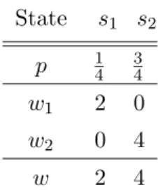
Example 1

One can imagine that 1 and 2 are agricultural producers and that w1, w2represents the

possible production of tomatoes during one year depending on the climate conditions s1 and s2. Note by the way that one could imagine that these agricultural

State s1 s2

p 1₂ 1₂

w1 2 0

w2 0 4

w 2 4

Table 1.1: Probability of the states for example 1.

Pareto optima separately with respect to tomatoes productions and potatoes produc-tions would apparently make sense in such a situation.

Here we are looking for individually rational Pareto optima X = (x1, x2) and Y =

(y1, y2). Clearly the individually rational Pareto optima (X, Y ) are characterized by:

Comonotonicity condition: x1 ≤ x2 and y1 ≤ y2.

Dominance: X�SSDw1 so x1 ≥ 0 and E(X) = E(w1) i.e. x1+ x2 = 2

Y_�SSD w2 so y1 ≥ 0 and E(Y ) = E(w2) i.e. y1+ y2 = 4.

Feasibility: x1 ≥ 0 and x2 ≥ 0, y1 ≥ 0 and y2 ≥ 0

x1 + y1 = 2, x2+ y2 = 4.

Hence direct computations give that the extreme IRPO’s are ((0, 2) , (2, 2)) and ((1, 1) , (1, 3)) so:

PIR = {(α2, 2α1+ α2) , (2α1+ α2, 2α1+ 3α2) , α1 ≥ 0, α2 ≥ 0, α1+ α2 = 1} .

Example 2

Note that we can write the initial situation as in table 1.3 by taking into account that the true states that will occur are s1 and s2, and not s1, s21, s22 and s23. So

Pareto optima will be X = (x1, x2) and Y = (y1, y2) or fictitious ˆX = (x1, x2, x2, x2)

and ˆY = (y1, y2, y2, y2), so the set PIR will now satisfy the polytope property:

State s1 s2

p 1₄ 3₄

w1 2 0

w2 0 4

w 2 4

Table 1.2: Initial probability of the states for example 2. State s1 s21 s22 s23 p 1₄ 1₄ 1₄ 1₄ ˆ w1 2 0 0 0 ˆ w2 0 4 4 4 ˆ w 2 4 4 4

Table 1.3: Converted to the uniform probability

Dominance: X�SSDw1 , x1 ≥ 0 and x1 + x2 ≥ 0, x1+ 2x2 ≥ 0,

E(X) = E(w1) i.e. x1+ 3x2 = 2

Y_�SSDw2 , y1 ≥ 0 and y1+ y2 ≥ 4, y1+ 2y2 ≥ 8,

E(Y ) = E(w2) i.e. y1+ 3y2 = 12.

Feasibility: x1 ≥ 0 and x2 ≥ 0, y1 ≥ 0 and y2 ≥ 0

x1+ y1 = 2, x2+ y2 = 4.

Hence direct computation gives that the extreme IRPO’s are ��0,2 3� , �2, 10 3�� and ��₁ 2, 1 2� , � 3 2, 7 2�� so: PIR = ��₁ 2α2, 2 3α1+ 1 2α2� , �2α1+ 3 2α2, 10 3α1+ 7 2α2� , α1 ≥ 0, α2 ≥ 0, α1+ α2 = 1�.

1.4.2 Revisiting the insurance example of Landsberger and Meilijson (1994)

Landsberger and Meilijson (1994) considered the following risky situation. In this example the following risky situation is considered. A risk averse agent owns a house worth 10$. The house is susceptible to a total loss with probability 1/10. The agent also owns 1$ in cash and a source of random income (stock) which pays 2$ or nothing with probability 1/2 each.

Fair insurance of the house is available but uncertainty associated with capital (stock) income is retained. Under fair insurance, the wealth positions of the insured and the insurer are given in table 1.4:

State s1 s2 s3 s4

Situation Stock pays zero Stock pays 2$ Stock pays zero Stock pays 2$ House-total loss House-total loss House intact House intact

Probability 0.05 0.05 0.45 0.45

Insured’s wealth

position X 10 12 10 12

Insurer’s wealth

position Z -9 -9 1 1

Table 1.4: Insurance example of Landsberger and Meilijson (1994).

We assume as Landsberger and Meilijson (1994) that both agents are strict strong risk averters. We intend to derive all the IRPO’s, while Landsberger and Meilijson (1994) just proposed one sharing rule through their specific algorithm.

Note that theorem 1.4.5 assumes that all the considered allocations are non-negative, so we need to prove that the results of theorem 1.4.5 remains valid if no boundedness constraints are imposed on the initial allocations and the Pareto optima. To this end, theorem 1.4.5 can be improved in the following way:

Theorem 1.4.6. Assume that the initial endowment of agent i is wi ∈ Rm and define

the IRP O’s as the allocations X = (X1, . . . , Xi, . . . , Xn) ∈ Rm×n such that �iXi =

�

iwi (:= w) and Xi�SSDwi ∀i, then the set PIR is the polytope of the feasible

allocations which are comonotone and satisfy the individually rational constraints. Proof: A simple examination of the proof of theorem 1.4.5 shows that it is just required to check that the set PIR is bounded.

We may assume since the probabilities are rational, that in fact we are considering the situation where all the states j = 1, ..., m are with probability 1/m.

So translating our problem in this setting, we may assume: w(1) _{≤ . . . ≤ w(j) ≤ . . . ≤ w(m).}

Thus we are looking for Xi, i = 1, ..., n such that from comonotonicity:

Xi(1) ≤ . . . ≤ Xi(j) ≤ . . . ≤ Xi(m) ∀i We know that for IRPO Xi, we have

Let σi : {1, ..., m}→ {1, ..., m} be the permutation such that,

wi(σi(1))≤ . . . ≤ wi(σi(j))≤ . . . ≤ wi(σi(m)).

Hence from dominance condition 2: Xi�SSDwi, we get:

�k

j=1Xi(j)≥�kj=1wi(σi(j)) ∀k ∈ {1, ..., m}.

Therefore for a given i, Xi(1) ≥ Minj wi(j), and then comonotonicity implies that

Xi(1) ≥ Minj wi(j) ∀i, hence the Xi’s are bounded from below. Condition 1

imme-diately leads to the fact that each Xi is bounded from above.

Considering that for a given i we have:

Xi(m) =�m_j=1wi(j)−�m−1_j=1 Xi(j)≤�m_j=1wi(j)− (m − 1)Minj wi(j).

Therefore from comonotonicity Xi ≤�m_j=1wi(j)−(m−1)Minjwi(j) which completes

the proof. ✷

Having proved the validity of our IRPO computation algorithm for the cases like Landsberger and Meilijson (1994)’s example, we apply our algorithm and we obtain the following two extreme points for the set of IRPO which are depicted in tables 1.5 and 1.6.

State s1 s2 s3 s4

X1 10 10.2 10.2 12

Z1 -9 -7.2 0.8 1

w 1 3 11 13

Table 1.5: First extreme point

State s1 s2 s3 s4

X2 10 10 10.22 12

Z2 -9 -7 0.78 1

w 1 3 11 13

Table 1.6: Second extreme point

In fact the first extreme point (X1, Z1) turns out to be the IRPO found by

Lands-berger and Meilijson (1994). Clearly any of the IRPO (i.e. any convex combination of (X1, Z1) and (X2, Z2)) allows both agents to reduce their risk compared to the initial

situation, but indeed while only the insurable risk was diversified using the insurance market, risk sharing allowed also social risks (stock risk) to be reduced.

1.5

Conclusion

In this paper, in case of multiple risks, we did adopt the idea that a natural way for insurance companies to optimally share risks is risk by risk Pareto-optimality. Our framework is based upon the well-known results in the one dimensional case characterizing Pareto-optimality as comonotonicity in case of strong risk aversion. Two main results are obtained in this work.

Due to the polytope structure of Pareto-optima and also of Individually Rational optima, we offer a simple computable method. First for deriving all Pareto-optima and second—in the not severely restrictive case of rational probabilities—for deriving all Individually Rational Pareto-optima. The method merely consists in systematically obtaining the finitely many extreme points of the respective polytopes. The method is illustrated using the numerical examples. Moreover the application of this approach in insurance industry is examined by computing all the IRPO’s of the Landsberger and Meilijson (1994)’s example.

Karl Borch. Equilibrium in a reinsurance market. Econometrica, 30(3):424–444, 1962. Guillaume Carlier, R-A Dana, and Alfred Galichon. Pareto efficiency for the concave order and multivariate comonotonicity. Journal of Economic Theory, 147(1):207– 229, 2012.

Alain Chateauneuf, Rose-Anne Dana, and Jean-Marc Tallon. Optimal risk-sharing rules and equilibria with choquet-expected-utility. Journal of Mathematical Eco-nomics, 34(2):191–214, 2000.

Michel Denuit and Jan Dhaene. Convex order and comonotonic conditional mean risk sharing. Insurance: Mathematics and Economics, 51(2):265 – 270, 2012. ISSN 0167-6687.

Louis Eeckhoudt, Christian Gollier, and Harris Schlesinger. Economic and financial decisions under risk. Princeton University Press, 2005.

Monique Florenzano, Cuong Le Van, and Pascal Gourdel. Finite dimensional con-vexity and optimization. Springer New York, 2001.

Michael Landsberger and Isaac Meilijson. Co-monotone allocations, bickel-lehmann dispersion and the arrow-pratt measure of risk aversion. Annals of Operations Research, 52(2):97–106, 1994.

Michael Ludkovski and Ludger R¨uschendorf. On comonotonicity of pareto optimal risk sharing. Statistics & Probability Letters, 78(10):1181–1188, 2008.

MATLAB. version 7.10.0 (R2010a). The MathWorks Inc., Natick, Massachusetts, 2010.

Comonotonic Monte Carlo and its

applica-tions in option pricing and quantification

of risk

1

Alain Chateauneuf, Mina Mostoufi, David Vyncke

Abstract

Monte Carlo (MC) simulation is a technique that provides approximate solutions to a broad range of mathematical problems. A drawback of the method is its high computational cost, especially in a high-dimensional setting, such as estimating the Tail Value-at-Risk for large portfolios or pricing basket options and Asian options. For these types of problems, one can construct an upper bound in the convex or-der by replacing the copula by the comonotonic copula. This comonotonic upper bound can be computed very quickly, but it gives only a rough approximation. In this paper we introduce the Comonotonic Monte Carlo (CoMC) simulation, by using the comonotonic approximation as a control variate. The CoMC is of broad appli-cability and numerical results show a remarkable speed improvement. We illustrate the method for estimating Tail Value-at-Risk and pricing basket options and Asian options when the logreturns follow a Black-Scholes model or a variance gamma model.

Keywords : Control Variate Monte Carlo, Comonotonicity, Option pricing. JEL classification: C02, C13, C15, G17.

2.1

Introduction

Monte Carlo (MC) simulation is a well known technique in different domains of math-ematics such as mathematical finance, see Glasserman (2003); Benninga (2014). The method is based on the estimation of the expectation of a real-valued random vari-able X by generating many independent and identically distributed samples of X, denoted X1, ..., Xn. The natural unbiased estimator for E(X) is then the sample

mean ¯Xn= 1_n n

�

i=1

Xi.

A typical application of the Monte Carlo method in finance is the estimation of the no-arbitrage price of a specific derivative security (e.g. a call option), which can be expressed as the expected value of its discounted payoff under the risk neutral measure. For instance the price at time t of a European call option with strike price K and maturity date T on an underlying with price process St can be obtained as

the expectation of its discounted payoff e−r(T −t)_(S

T − K)+ under the risk-neutral

probability Q,

EC(K, T, t) = EQ[e−r(T −t)_(S

T − K)+].

For the computation of this price by Monte Carlo simulation, we generate a large number of price paths ST and compute the discounted payoffs and their sample mean.

The obtained result is an unbiased estimate of the option price.

Another application of the Monte Carlo method in finance is estimating risk measures, such as Tail Value-at-Risk. The Tail Value-at-Risk of a portfolio at the probability level p is the arithmetic average of its quantiles from the threshold p to 1. The Monte Carlo method estimates these quantiles by generating a huge number of portfolio val-ues for which the exceedance probabilities P r[X ≥ x] = E[I(X ≥ x)] are computed, where I(.) denotes the indicator function. A classical interpolation and inversion then gives an estimate for the quantile.

The main shortcoming of the Monte Carlo method is its high computational cost. By the Central Limit Theorem, if X1, ..., Xn have finite variance σ2, then ¯Xn is

approx-imately Gaussian and Var( ¯Xn)=σ

2

n. Consequently, the standard error of the crude

Monte Carlo estimate is of order O(_√1

n) and thus, to double the precision, one must

run four times the number of simulations. Alternatively, strategies for reducing σ should be considered.

Several variance reduction techniques can be used in companion with the Monte Carlo method, such as antithetic variables, control variates and importance sampling. A