HAL Id: hal-00160051
https://hal.archives-ouvertes.fr/hal-00160051
Submitted on 4 Jul 2007
HAL is a multi-disciplinary open access
archive for the deposit and dissemination of
sci-entific research documents, whether they are
pub-lished or not. The documents may come from
teaching and research institutions in France or
abroad, or from public or private research centers.
L’archive ouverte pluridisciplinaire HAL, est
destinée au dépôt et à la diffusion de documents
scientifiques de niveau recherche, publiés ou non,
émanant des établissements d’enseignement et de
recherche français ou étrangers, des laboratoires
publics ou privés.
How to use the Scuba Diving metaphor to solve problem
with neutrality ?
Philippe Collard, Sébastien Verel, Manuel Clergue
To cite this version:
Philippe Collard, Sébastien Verel, Manuel Clergue. How to use the Scuba Diving metaphor to solve
problem with neutrality ?. ECAI’2004, Aug 2004, Valencia, Spain. pp.166-170. �hal-00160051�
hal-00160051, version 1 - 4 Jul 2007
How to use the Scuba Diving metaphor to solve problem
with neutrality ?
Collard Philippe and Verel S´ebastien and Clergue Manuel
1Abstract. We proposed a new search heuristic using the scuba
div-ing metaphor. This approach is based on the concept of evolvability and tends to exploit neutrality which exists in many real-world prob-lems. Despite the fact that natural evolution does not directly select for evolvability, the basic idea behind the scuba search heuristic is to explicitly push evolvability to increase. A comparative study of the scuba algorithm and standard local search heuristics has shown the advantage and the limitation of the scuba search. In order to tune neutrality, we use the N Kq fitness landscapes and a family of travel-ling salesman problems (TSP) where cities are randomly placed on a lattice and where travel distance between cities is computed with the Manhattan metric. In this last problem the amount of neutrality varies with the city concentration on the grid ; assuming the concentration below one, this TSP reasonably remains a NP-hard problem.
1
Introduction
In this paper we propose an heuristic called Scuba Search that al-lows us to exploit the neutrality that is present in many real-world problems. This section presents the interplay between neutrality in search space and metaheuristics. Section 2 describes the Scuba Search heuristic in details. In order to illustrate efficiency and limit of this heuristic, we use the N Kq fitness landscapes and a travelling salesman problem (TSP) on diluted lattices as a model of neutral search space. These two problems are presented in section 3. Experi-ment results are given in section 4 where comparisons are made with two hill climbing heuristics. In section 5, we point out advantage and shortcoming of the approach; finally, we summarize our contribution and present plans for a future work.
1.1
Neutrality
The metaphor of an ’adaptative landscape’ introduced by
S. Wright [14] has dominated the view of adaptive evolution: an up-hill walk of a population on a mountainous fitness landscape in which it can get stuck on suboptimal peaks. Results from molecular evolu-tion has changed this picture: Kimura’s model [7] assumes that the overwhelming majority of mutations are either effectively neutral or lethal and in the latter case purged by negative selection. This as-sumption is called the neutral hypothesis. Under this hypothesis, the dynamics of populations evolving on such neutral landscapes are dif-ferent from those on adaptive landscapes: they are characterized by long periods of fitness stasis (population is situated on a ’neutral net-work’) punctuated by shorter periods of innovation with rapid fitness increase. In the field of evolutionary computation, neutrality plays
1Laboratoire I3S, Universit´e de Nice-Sophia Antipolis, France, Email:{pc,
verel, clerguem}@i3s.unice.fr
an important role in real-world problems: in design of digital circuits [12], in evolutionary robotics [5]. In those problems, neutrality is im-plicitly embedded in the genotype to phenotype mapping.
1.2
Evolvability
Evolvability is defined by Altenberg [13] as “the ability of random variations to sometimes produce improvement”. This concept refers to the efficiency of evolutionary search; it is based upon the work by Altenberg [1]: “the ability of an operator/representation scheme to produce offspring that are fitter than their parents”. As enlighten by Turney [11] the concept of evolvability is difficult to define. As he
puts it: “if s and s′are equally fit, s is more evolvable than s′if the
fittest offspring of s is more likely to be fitter than the fittest offspring
of s′”. Following this idea we define evolvability as a function (see
section 2.2).
2
Scuba Search
The Scuba Search, heuristic introduced in this section, exploits neu-trality by combining local search heuristic with navigating the neutral neighborhood of states.
2.1
The Scuba Diving Metaphor
Keeping the landscape as a model, let us imagine this landscape with peaks (local optima) and lakes (neutral networks). Thus, the land-scape is bathed in an uneven sea; areas under water represent non-viable solutions. So there are paths from one peak to another one for a swimmer. The key, of course, remains to locate an attractor which represents the system’s maximum fitness. In this context, the prob-lem is to find out how to cross a lake without global information. We use the scuba diving metaphor as a guide to present principles of the so-called scuba search (SS). This heuristic is a way to deal with the problem of crossing in between peaks. then we avoid to be trapped in the vicinity of local optima. The problem is to get to know what drives the swimmer from one edge of the lake to the opposite one? Up to the classic view a swimmer drifts at the surface of a lake. The new metaphor is a scuba diving seeing the world above the water surface. We propose a new heuristic to cross a neutral net getting information above-the-surface (ie. from fitter points in the neighborhood).
2.2
Scuba Search Algorithm
Despite the fact that natural evolution does not directly select for evolvability, there is a dynamic pushing evolvability to increase [11]. The basic idea behind the SS heuristic is to explicitly push evolv-ability to increase. Before presenting this search algorithm, we need
to introduce a new type of local optima, the local-neutral optima. Indeed with SS heuristic, local-neutral optima will allow transition from neutral to adaptive evolution. So evolvability will be locally
op-timized. Given a search spaceS and a fitness function f defined on
S, some more precise definitions follow.
Definition: A neighborhood structure is a functionV : S → 2S
that assigns to every s ∈ S a set of neighbors V(s) such that s ∈
V(s).
Definition: The evolvability of a solution s is the function evol
that assigns to every s∈ S the maximum fitness from the
neighbor-hoodV(s): ∀s ∈ S, evol(s) = max{f (s′) | s′ ∈ V(s)}.
Definition: For every fitness function g, neighborhood structure
W and genotype s, the predicate isLocal is defined as: isLocal(s, g, W) = (∀s′ ∈ W(s), g(s′) ≤ g(s)).
Definition: For every s∈ S, the neutral set of s is the set N (s) = {s′ ∈ S | f (s′) = f (s)}, and the neutral neighborhood of s is the
setVn(s) = V(s) ∩ N (s).
Definition: For every s ∈ S, the neutral degree of s, noted Degn(s), is the number of neutral neighbors of s, Degn(s) = #Vn(s) − 1.
Definition: A solution s is a local maximum iff isLocal(s, f, V).
Definition: A solution s is a local-neutral maximum iff
isLocal(s, evol, Vn).
Scuba Search use two dynamics one after another (see algo.1). The first one corresponds to a neutral path. At each step the scuba diving remains under the water surface driven by the hands-down fit-nesses; that is fitter fitness values reachable from one neutral neigh-bor. At that time the flatCount counter is incremented. When the div-ing reaches a local-neutral optimum, i.e. when all the fitnesses reach-able from one neutral neighbor are selectively neutral or disadvanta-geous, the neutral path stops and the diving starts up the Invasion-of-the-Land. Then the gateCount counter increases. This process goes along, switching between Conquest-of-the-Waters and Invasion-of-the-Land, until a local optimum is reached.
Algorithm 1 Scuba Search
flatCount← 0, gateCount ← 0
Choose initial solution s∈ S
repeat
while not isLocal(s, evol, Vn) do
M = max{evol(s′) | s′∈ Vn(s) − {s}}
if evol(s) < M then
choose s′ ∈ Vn(s) such that evol(s′) = M
s← s′, flatCount← flatCount +1
end if end while
choose s′ ∈ V(s) − Vn(s) such that f (s′) = evol(s)
s← s′, gateCount← gateCount +1
until isLocal(s, f, V)
3
Models of Neutral Seach Space
In order to study the Scuba Search heuristic we have to use land-scapes with a tunable degree of neutrality.
3.1
The NKq fitness Landscape
The N Kq fitness landscapes family proposed by Newman et al. [9] has properties of systems undergoing neutral selection such as
RNA sequence-structure maps. It is a generalization of the N K-landscapes proposed by Kauffman [6] where parameter K tunes the ruggedness and parameter q tunes the degree of neutrality.
3.1.1 Definition and properties
The fitness function of a N Kq-landscape [9] is a function f :
{0, 1}N → [0, 1] defined on binary strings with N loci. Each
lo-cus i represents a gene with two possible alleles,0 or 1. An ’atom’
with fixed epistasis level is represented by a fitness components
fi : {0, 1}K+1 → [0, q − 1] associated to each locus i. It depends
on the allele at locus i and also on the alleles at K other epistatic loci
(K must fall between0 and N − 1). The fitness f (x) of x ∈ {0, 1}N
is the average of the values of the N fitness components fi:
f(x) = 1 N(q − 1) N X i=1 fi(xi; xi1, . . . , xiK)
where{i1, . . . , iK} ⊂ {1, . . . , i − 1, i + 1, . . . , N }. Many ways
have been proposed to choose the K other loci from N loci in the genotype. Two possibilities are mainly used: adjacent and random neighborhoods. With an adjacent neighborhood, the K genes near-est to the locus i are chosen (the genotype is taken to have periodic boundaries). With a random neighborhood, the K genes are chosen
randomly on the genotype. Each fitness component fi is specified
by extension, ie an integer number yi,(xi;xi1,...,xiK)from[0, q − 1]
is associated with each element(xi; xi1, . . . , xiK) from {0, 1}
K+1.
Those numbers are uniformly distributed in the interval[0, q−1]. The
parameters of N Kq-landscape tune ruggedness and neutrality of the landscape [4]. The number of local optima is linked to the parameter
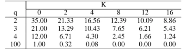
K. The largest number is obtained when K takes its maximum value N− 1. The neutral degree (see tab. 1) decreases as q or K increases.
The maximal degree of neutrality appears when q takes value2.
Table 1. Average neutral degree on N Kq-landscapes with N = 64
per-forms on50000 genotypes K q 0 2 4 8 12 16 2 35.00 21.33 16.56 12.39 10.09 8.86 3 21.00 13.29 10.43 7.65 6.21 5.43 4 12.00 6.71 4.30 2.45 1.66 1.24 100 1.00 0.32 0.08 0.00 0.00 0.00 3.1.2 Parameters setting
All the heuristics used in our experiments are applied to a same
instance of N Kq fitness landscapes2 with N = 64. The
neigh-borhood is the classical one-bit mutation neighneigh-borhood: V(s) =
{s′ | Hamming(s′, s) ≤ 1}. For each triplet of parameters N , K and q,103runs were performed.
3.2
The Travelling Salesman Problem on randomly
diluted lattices
The family of TSP proposed by Chakrabarti [3] is an academic benchmark that allows to test our ideas. These problems do not reflect the true reality but is a first step towards more real-life benchmarks. We use these problems to incorporate a tunable level of neutrality into TSP search spaces.
3.2.1 Definition and properties
The travelling salesman problem is a well-known combinatorial op-timization problem: given a finite number N of cities along with the cost of travel between each pair of them, find the cheapest way of vis-iting all the cities and returning to your starting point. In this paper we use a TSP defined on randomly dilute lattices. The N cities randomly
occupy lattice sites of a two-dimentional square lattice (L× L). We
use the Manhattan metric to determine the distance between two cities. The lattice occupation concentration (i.e. the fraction of sites
occupied) isL2N. As the concentration is related to the neutral degree,
we note T SP n such a problem with concentration n. For n= 1, the
problem is trivial as it can be reduced to the one-dimensional TSP. As n decreases from unity the problem becomes nontrivial: the dis-creteness of the distance of the path connecting two cities and the angle which the path makes with the Cartesian axes, tend to
disap-pear. Finally, as n→ 0, the problem can be reduced to the standard
two-dimensional TSP. As Chakrabarti [3] stated: “it is clear that the
problem crosses from triviality (for n= 1) to NP-hard problem at a
certain value of n. We did not find any irregularity|...| at any n. The
crossover from triviality to NP-hard problem presumably occurs at
n= 1.”
The idea is to discretize the possible distances, through only al-lowing each distance to take one of D distances. Varying this terrace parameter D from an infinite value (corresponding to the standard
TSP), down to the minimal value of 1 thus decreases the number
of possible distances, so increasing the fraction of equal fitness
neu-tral solutions. So, parameter n = N
L2 of the T SP n tunes both the
concentration and the neutral degree (see fig. 1). In the remaining of this paper we consider T SP n problems where n stands in the range
[0, 1]. 0.1 0.12 0.14 0.16 0.18 0.2 0.22 0.24 10 20 30 40 50 60 70 100
Proportion of neutral neighbors
L
Figure 1. Average proportion of neutral neighbors on T SP n as function of L, for N= 64 (values are computing from 50000 random solutions)
3.2.2 Parameters setting
All the heuristics used in our experiments are applied to a same
in-stance of T SP n. The search spaceS is the set of permutations of
{1, . . . , N }. The neighborhood is induced by the classical 2-opt
mu-tation operator:V(s) = {s′ | s′ = 2-opt(s)}. The size of
neighbor-hood is thenN(N−3)2 . For each value of L,500 runs were performed.
4
Experiment Results
4.1
Algorithm of Comparison
Two Hill Climbing algorithms are used for comparison.
4.1.1 Hill Climbing
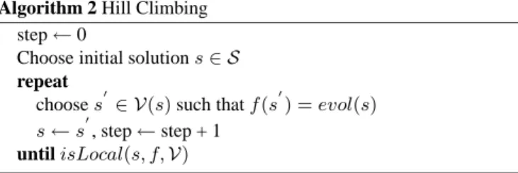
The simplest type of local search is known as Hill Climbing (HC) when trying to maximize a solution. HC is very good at exploit-ing the neighborhood; it always takes what looks best at that time. But this approach has some problems. The solution found depends on the initial solution. Most of the time, the found solution is only a local optima. We start off with a probably suboptimal solution. We then look in the neighborhood of that solution to see if there is some-thing better. If so, we adopt this improved solution as our current best choice and repeat. If not, we stop assuming that the current solution is good enough (local optimum).
Algorithm 2 Hill Climbing
step← 0
Choose initial solution s∈ S
repeat
choose s′∈ V(s) such that f (s′) = evol(s)
s← s′, step← step + 1
until isLocal(s, f, V)
4.1.2 Hill Climbing Two Steps
Hill Climber can be extended in many ways. Hill Climber two Step (HC2) exploits a larger neighborhood of stage 2. The algorithm is
nearly the same as HC. HC2 looks in the extended neighborhood of
stage two of the current solution to see if there is something better. If
so, HC2 adopts the solution in the neighborhood of stage one which
can reach a best solution in the extended neighborhood. If not, HC2
stop assuming the current solution is good enough. So, HC2 can
avoid more local optimum than HC. Before presenting the algorithm 3 we must introduce the following definitions:
Definition: The extended neighborhood structure3fromV is the
functionV2(s) = ∪
s1∈V(s)V(s1)
Definition: evol2is the function that assigns to every s∈ S the
maximum fitness from the extended neighborhoodV2(s). ∀s ∈ S,
evol2(s) = max{f (s′)|s′∈ V2(s)}
Algorithm 3 Hill Climbing (Two Steps)
step← 0
Choose initial solution s∈ S
repeat
if evol(s) = evol2(s) then
choose s′ ∈ V(s) such that f (s′) = evol2(s)
else
choose s′ ∈ V(s) such that evol(s′) = evol2(s)
end if
s← s′, step← step + 1
until isLocal(s, f, V2)
4.2
Performances
In this section we present the average fitness found using each heuris-tic on both N K and T SP problems.
4.2.1 NKq Landscapes
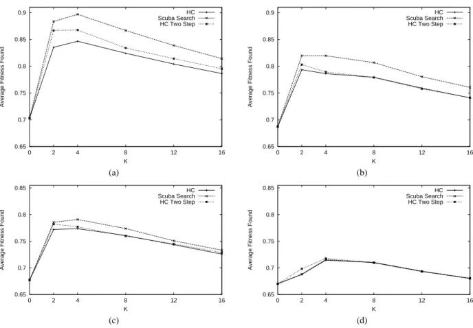
Figure 2 shows the average fitness found respectively by each of the three heuristics as a function of the epistatic parameter K for different values of the neutral parameter q. In the presence of neu-trality, according to the average fitness, Scuba Search outperforms Hill Climbing and Hill Climbing two steps. Let us note that with
high neutrality (q = 2 and q = 3), the difference is still more
significant. Without neutrality (q= 100) all the heuristics are nearly
equivalent. The Scuba Search have on average better fitness value
for q = 2 and q = 3 than hill climbing heuristics. This
heuris-tic benefits in N Kq from the neutral paths to reach the highest peaks.
4.2.2 TSPn Problems
Table 2 shows the fitness performances of heuristics on T SP n land-scapes. The average and the best fitness found by SS are always above the ones for HC. As for N Kq landscapes, the difference is
more important when neutrality is more significant (L = 10 and
L = 20). Performances of SS are a little better for L = 10 and L= 20 and a little less for L = 30 and L = 100. Let us also note
that standart deviation is still smaller for SS.
Table 2. Average and standart deviation of fitness found on T SP n (N = 64) performed on 500 independants runs. Best fitness found is putted in
brackets heurist L 10 20 30 100 HC 1015(90) 19310(164) 29313(256) 87244(770) SS 934(84) 1808(162) 28112(254) 85741(764) HC2 958(86) 18415(162) 28218(252) 85461(764)
4.3
Evaluation cost
4.3.1 NKq LandscapesTable 3 shows the number of evaluations for the different heuristics. For all the heuristics, the number of evaluations decreases with K. The evaluation cost decreases as ruggedness increases. For HC and
HC2, the evaluation cost increases with q. For HC and HC2, more
neutral the landscape is, smaller the evaluation cost. Conversely, for
SS the cost decreases with q. At each step the number of
evalua-tions is N for HC and N(N−1)2 for HC2. So, the cost depends on
the length of adaptive walk of HC and HC2 only. The evaluation
cost of HC and HC2 is low when local optima are nearby (i.e. in
rugged landscapes). For SS, at each step, the number of evaluations is(1 + Degn(s))N which decreases with neutrality. So, the
num-ber of evaluations depends both on the numnum-ber of steps in SS and on the neutral degree. The evaluation cost of SS is high in neutral landscape.
Table 3. Average number of evaluations on N Kq-landscape with N= 64
K q 0 2 4 8 12 16 HC 991 961 807 613 491 424 SS 2 35769 23565 15013 8394 5416 3962 HC2 29161 35427 28038 19192 15140 12374 HC 1443 1159 932 694 546 453 SS 3 31689 17129 10662 6099 3973 2799 HC2 42962 37957 29943 20486 15343 12797 HC 1711 1317 1079 761 614 500 SS 4 22293 9342 5153 2601 1581 1095 HC2 52416 44218 34001 22381 18404 14986 HC 2102 1493 1178 832 635 517 SS 100 4175 1804 1352 874 653 526 HC2 63558 52194 37054 24327 18260 15271 4.3.2 TSPn Problems
Table 4 shows the number of evaluations on T SP n. Scuba Search
uses a larger number of evaluations than HC (nearly200 times on
average) and smaller than HC2 (nearly 12 times on average). As
ex-pected, for SS the evaluation cost decreases with L and so the
neu-trality of landscapes; whereas it increase for HC and HC2.
Land-scape seems more rugged when L is larger.
Table 4. Average number of evaluations (x106) on the family of T SP n
problems with N= 64 L 10 20 30 100 HC 0.0871 0.101 0.105 0.117 SS 25.3 20.2 16.6 13.0 HC2 183.7 204.0 211.4 230.5
5
Discussion and conclusion
According to the average fitness found, Scuba Search outperforms the others local search heuristics on both N Kq and T SP n as soon as neutrality is sufficient. However, it should be wondered whether effi-ciency of Scuba Search does have with the greatest number of eval-uations. The number of evaluations for Scuba Search is lesser than
the one for HC2. This last heuristic realizes a larger exploration of
the neighborhood than SS: it pays attention to neighbors with same fitness and all the neighbors of the neighborhood too. However the average fitness found is worse than the one found by SS. So, consid-ering the number of evaluations is not sufficient to explain good per-formance of SS. Whereas there is premature convergence towards
local optima with HC2, SS realizes a better compromise between
exploration and exploitation by examining neutral neighbors. The main idea behind Scuba Search heuristic is to try to explic-itly optimize evolvability on a neutral network before performing a qualitative step using a local search heuristic. If evolvability is almost constant on each neutral network, for instance as in the well-known Royal-Road landscape [8], SS cannot perform neutral moves to in-crease evolvability and then have the same dynamic than HC. In this kind of problem, scuba search fails in all likehood.
In order to reduce the evaluation cost of SS, one solution would be to choose a “cheaper” definition for evolvability: for example, the best fitness of n neighbors randomly chosen or the first fitness of neighbor which improves the fitness of the current genotype. An-toher solution would be to change either the local search heuristic which evolvability or the one which allows to jump to a fitter solu-tion. For instance, we could use Simulated Annealing or Tabu Search
0.65 0.7 0.75 0.8 0.85 0.9 0 2 4 8 12 16
Average Fitness Found
K HC Scuba Search HC Two Step 0.65 0.7 0.75 0.8 0.85 0.9 0 2 4 8 12 16
Average Fitness Found
K HC Scuba Search HC Two Step (a) (b) 0.65 0.7 0.75 0.8 0.85 0 2 4 8 12 16
Average Fitness Found
K HC Scuba Search HC Two Step 0.65 0.7 0.75 0.8 0.85 0 2 4 8 12 16
Average Fitness Found
K
HC Scuba Search HC Two Step
(c) (d)
Figure 2. Average fitness found on N Kq-landscapes as function of K, for N= 64 and q = 2 (a), q = 3 (b), q = 4 (c), q = 100 (d) to optimize neutral network then jump to the first improvement met
in the neighborhood.
This paper represents a first step demonstrating the potential inter-est in using the scuba search heuristic to optimize neutral landscape. Obviously we have to compare performances of this metaheuristic with other metaheuristics adapted to neutral landscape as Netcrawler [2] or extrema selection [10]. All these strategies use the neutrality in different ways to find good solution and may not have the same performances on all problems. SS certainly works well when evolv-ability on neutral networks can be optimized.
REFERENCES
[1] Lee Altenberg, ‘The evolution of evolvability in genetic programming’, in In Kinnear, Kim (editor). Advances in Genetic Programming.
Cam-brige, MA, pp. 47–74. The MIT Press, (1994).
[2] Lionel Barnett, ‘Netcrawling - optimal evolutionary search with neutral networks’, in IEEE Congress on Evolutionary Computation 2001, pp. 30–37, COEX, World Trade Center, 159 Samseong-dong, Gangnam-gu, Seoul, Korea, (2001). IEEE Press.
[3] A. Chakraborti and B.K. Chakrabarti, ‘The travelling salesman prob-lem on randomly diluted lattices: Results for small-size systems’, The
European Physical Journal B, 16(4), 677–680, (2000).
[4] N. Geard, J. Wiles, J. Hallinan, B. Tonkes, and B. Skellett, ‘A compar-ison of neutral landscapes – nk, nkp and nkq’, in Proceedings of the
IEEE Congress on Evolutionary Computation, (2002).
[5] N. Jakobi, P. Husbands, and I. Harvey, ‘Noise and the reality gap: The use of simulation in evolutionary robotics’, Lecture Notes in Computer
Science, 929, 704–801, (1995).
[6] S. A. Kauffman, “The origins of order”. Self-organization and
selec-tion in evoluselec-tion, Oxford University Press, New-York, 1993.
[7] M. Kimura, The Neutral Theory of Molecular Evolution, Cambridge University Press, Cambridge, UK, 1983.
[8] M. Mitchell, S. Forrest, and J. H. Holland, ‘The royal road for ge-netic algorithms: Fitness landscape and GA performance’, in
Pro-ceedings of the First European Conference on Artificial Life, eds., F.J
Varela and P. Bourgine, pp. 245–254, Cambridge, MA, (1992). MIT Press/Bradford Books.
[9] M. Newman and R. Engelhardt, ‘Effect of neutral selection on the evo-lution of molecular species’, in Proc. R. Soc. London B., volume 256, pp. 1333–1338, (1998).
[10] T.C. Stewart, ‘Extrema selection: Accelerated evolution on neutral net-works’, in IEEE Congress on Evolutionary Computation 2001, COEX, World Trade Center, 159 Samseong-dong, Gangnam-gu, Seoul, Korea, (2001). IEEE Press.
[11] Peter D. Turney, ‘Increasing evolvability considered as a large scale trend in evolution’, in GECCO’99 : Proceedings of the 1999
Ge-netic and Evolutionary Computation Conference, Workshop Pro-gram on evolvability, eds., Paul Marrow, Mark Shackleton, Jose-Luis
Fernandez-Villacanas, and Tom Ray, pp. 43–46, (1999).
[12] Vesselin K. Vassilev and Julian F. Miller, ‘The advantages of landscape neutrality in digital circuit evolution’, in ICES, pp. 252–263, (2000). [13] G. P. Wagner and L. Altenberg, ‘Complexes adaptations and the
evolu-tion of evolvability’, in Evoluevolu-tion, pp. 967–976, (1996).
[14] S. Wright, ‘The roles of mutation, inbreeding, crossbreeding, and selec-tion in evoluselec-tion’, in Proceedings of the Sixth Internaselec-tional Congress of