HAL Id: cea-02339334
https://hal-cea.archives-ouvertes.fr/cea-02339334
Submitted on 15 Dec 2019HAL is a multi-disciplinary open access archive for the deposit and dissemination of sci-entific research documents, whether they are pub-lished or not. The documents may come from teaching and research institutions in France or abroad, or from public or private research centers.
L’archive ouverte pluridisciplinaire HAL, est destinée au dépôt et à la diffusion de documents scientifiques de niveau recherche, publiés ou non, émanant des établissements d’enseignement et de recherche français ou étrangers, des laboratoires publics ou privés.
Optimized non-parametric fragility curve estimation
based on intensity measure data clustering and
parametric model averaging
K. Trevlopoulos, C. Feau, I. Zentner
To cite this version:
K. Trevlopoulos, C. Feau, I. Zentner. Optimized non-parametric fragility curve estimation based on intensity measure data clustering and parametric model averaging. 16Th European Conference On Earthquake Engineering, Jun 2018, Thessalonique, Greece. �cea-02339334�
1
Parametric models averaging for optimized non-parametric fragility curve estimation 1
based on intensity measure data clustering 2
3
Konstantinos Trevlopoulosa1, Cyril Feaua, Irmela Zentnerb,c 4
aDEN - Service d’études mécaniques et thermiques (SEMT), CEA, Université Paris-Saclay, 5
F-91191 Gif-sur-Yvette, France 6
bEDF R&D, EDF Lab Paris-Saclay, 7 Bvd Gaspard Monge, 91120 Palaiseau, France 7
cIMSIA, UMR CNRS-EDF-CEA-ENSTA ParisTech, Université Paris-Saclay, France 8
ABSTRACT 9
Seismic fragility curves give the probability of exceedance of the threshold of a damage state 10
of a structure, or a non-structural component, conditioned on the intensity measure of the 11
seismic motion. Typically, fragility curves are constructed parametrically assuming a 12
lognormal shape. In some cases, which cannot be identified a priori, differences may be 13
observed between non-parametric fragility curves, evaluated empirically based on a large 14
number of seismic response analyses, and their estimations via the lognormal assumption. 15
Here, we present an optimized Monte Carlo procedure for derivation of non-parametric fragility 16
curves. This procedure uses clustering of the intensity measure data to construct the non-17
parametric curve and parametric models averaging for optimized assessment. In simplified 18
case studies presented here as illustrative applications, the developed procedure leads to a 19
fragility curve with reduced bias compared to the lognormal curve and to reduced confidence 20
intervals compared to an un-optimized Monte Carlo-based approach. In the studied cases, 21
this procedure proved to be efficient providing reasonable estimations even with as few as 22
100 seismic response analyses. 23
1Corresponding author. E-mail address: [email protected]. Present address: French
Alternative Energies and Atomic Energy Commission (CEA), DEN, 13108 Saint-Paul-lez-Durance CEDEX, France
2 24
Keywords: Seismic fragility curve; Non-parametric curve; Optimization; Data Clustering; 25
Parametric Models Averaging 26
1 INTRODUCTION 27
A multitude of procedures is now available for probabilistic seismic assessment of structures 28
[1]. Most notable is the framework by Yang et al. [2], which was the basis for the FEMA P-58 29
guidelines [3]. Here, we focus on fragility curves giving the probability to exceed a damage 30
state threshold conditioned on a measure of the intensity of the seismic motion, such as the 31
fragility curves defined in [4]. Such fragility curves are used for probabilistic assessment of 32
seismic risk [5] for structures and non-structural components in nuclear installations [6] and 33
critical civil infrastructure, such as hospitals and ports of major urban areas in earthquake 34
prone regions [7]. They can also be used to evaluate the impact of construction details on the 35
structural performance of installations under seismic excitations [8–11] and in rapid response 36
applications for risk management during a seismic crisis [12]. The use of fragility curves is not 37
limited to earthquake-related problems, they are also used in the case of other types of loading 38
such as wind [13]. 39
The classical formulation of a fragility curve makes the hypothesis that the curve 40
follows a lognormal shape. D’Ayala et al. [14] and FEMA [3] describe a series of procedures 41
for analytical fragility curve estimation, which are commonly applied. Analytical fragility curve 42
estimation is based on Engineering Demand Parameter (EDP) observations as a function of 43
the Intensity Measure (IM). In order to obtain such observations, either cloud analysis, 44
Incremental Dynamic Analysis (IDA) [15] or Multiple Stripes Analysis (MSA) [16] may be 45
performed. Linear regression [17] is a common method for lognormal fragility curve estimation. 46
The most well established methods for adjusting a lognormal fragility curve to observations 47
from IDA or MSA were developed by Baker [4] and are based on the method of moments and 48
Maximum Likelihood Estimation (MLE), respectively. 49
3
However, Mai et al. [18] observed differences between non-parametric fragility curves 50
based on kernel density estimation and lognormal fragility curves according to different 51
procedures and highlighted the effect of the derivation procedure on lognormal fragility curves. 52
Noh et al. [19] also used kernel smoothing in order to construct non-parametric fragility curves 53
showing that this can be an efficient solution when using sparse data. Lallement et al. [20] 54
consider non-parametric fragility curves more truthful representations of observations and 55
construct curves based on generalized additive models and Gaussian kernel smoothing. 56
Furthermore, in [21], lognormal fragility curves for structural components did not represent 57
effectively observations from simulations of the seismic response of a bridge. 58
The simplest construction of a non-parametric curve puts the EDP observations in bins 59
according to the corresponding IM and estimates empirically the probability of exceeding the 60
damage state threshold for every bin [22]. In practice, due to the prohibitive computational 61
cost of most nonlinear mechanical models, the development of numerically efficient methods 62
is required to evaluate such curves using a minimal number of computations. 63
Here, we propose a procedure based on Monte-Carlo (MC) simulations, which uses 64
Parametric Models Averaging (PMA) in order to optimize the computation of non-parametric 65
fragility curves, which are constructed based on k-means clustering [23] of the intensity 66
measure data. Optimization is employed in order to obtain reduced confidence fragility curve 67
intervals compared to the empirical estimations with an un-optimized MC approach. The key 68
elements of the optimization are: (i) the EDP observations are computed with seismic 69
response analyses using synthetic accelerograms, which are realizations of stochastic 70
processes, (ii) the non-parametric fragility curve is expressed through the law of total 71
probability as the weighted average of parametric fragility curves, each one of which is 72
estimated based on the synthetic ground motions generated by a stochastic process. In the 73
optimized approach, two alternative parametric models per process are proposed for the 74
probability of exceedance of the damage state threshold. Finally, the range of applicability of 75
each parametric model per process is analyzed. 76
4
To illustrate the proposed methodology, “simple” stochastic processes are defined 77
generating synthetic accelerograms based on original seed acceleration records (Section 2). 78
The generation results in a set of synthetic accelerograms reproducing the ground motion 79
variability observed in the original set of ground motion records. The procedure for selection 80
of the original seed records defining the processes is out of the scope of this work. Here, for 81
simplicity, the initial set of ground motions are selected using magnitude and distance as 82
criteria. 83
Here, the non-parametric fragility curves are estimated using as IM the Peak Ground 84
Acceleration (PGA) or the spectral acceleration at the frequency of an oscillator. However, the 85
developed procedure is independent of the selected IM. In the studied cases, the 95 % 86
confidence interval (CI) of the estimated fragility curves is significantly reduced due to the 87
optimization. Moreover, the bias of the fragility curves according to the optimization is tolerable 88
or negligible with respect to the reference curve obtained with a very large number of 89
observations, as long as the applicability recommendations are respected. 90
2 SYNTHETIC GROUND MOTION GENERATION 91
2.1 Motivation 92
Here, synthetic ground motions are employed in order to cover the range of IMs of 93
interest and eventually obtain fragility curves based on IM clustering that are well discretized. 94
Moreover, synthetic ground motions are used in order to exploit the statistical characteristics 95
of the ground motions given by a process, such as the distribution of the IMs of the generated 96
motions, in the context of the optimization of the computation of non-parametric fragility 97
curves. A "simple" synthetic ground motion generator is developed, which reproduces the 98
spectral variability of recorded accelerograms, because no hypothesis is introduced 99
concerning their frequency content. Moreover, the original recorded accelerograms are 100
selected from the European Strong Motion Database [24,25] using simple criteria, i.e. 5.5 < M 101
< 6.5 and R < 20 km. Selection of the original ground motions is out of the scope of this study. 102
5
It is worth noting that the main idea in the PMA methodology is that the synthetic ground 103
motion database consists of realizations of several stochastic processes. Therefore the 104
methodology herein could be used theoretically in conjunction with other procedures for 105
synthetic ground motion generation defining stochastic processes, such as the model in 106
Rezaeian and Der Kiureghian [26]. A study of the effect of the ground motion generator is out 107
of the scope of this article. As far as the most appropriate generator is concerned, that depends 108
on the problem at hand and the available data (e.g. response spectra, acceleration records, 109
see [1]). 110
2.2 Synthetic Ground Motion Generation Process 111
The generation process in this framework begins with retaining the FFT amplitude of 112
every real record in the original data set, replacing the phases with a vector of uniformly 113
distributed random values, computing the new ground motion via inverse FFT and imposing a 114
modulation function. The result is a series of unadjusted synthetic ground motions, which are 115
subsequently adjusted so that they are on average “spectrally equivalent” with the ground 116
motion records in the sense of acceleration response spectra. The i-th accelerogram (i = {1, 117
..., Nr}) in a data set of Nr ground motion records may be expressed with Equation 1. The 118
amplitudes (Ar,im) of the i-th real record (𝛼𝑟,𝑖(𝑡)) are computed with the FFT algorithm and are
119
used in combination with random phase (φs,ijm) in order to compute the j-th realization of a
120
stationary Gaussian process (Equation 2). 121 122 𝛼𝑟,𝑖(𝑡) = ∑ (𝐴𝑟,𝑖𝑚𝑠𝑖𝑛(𝜔𝑚+ 𝜑𝑟,𝑖𝑚)) 𝑛 𝑚=1 123 𝑖 = {1, … , 𝑁𝑟} (1) 124 125 𝛼𝑠,𝑖𝑗(𝑡) = ∑ (𝐴𝑟,𝑖𝑚𝑠𝑖𝑛(𝜔𝑚+ 𝜑𝑠,𝑖𝑗𝑚)) 𝑛 𝑚=1 126 𝑖 = {1, … , 𝑁𝑟}, 𝑗 = {1, … , 𝑁𝑠} (2) 127
6 128
where φs,ijm is the phase which is assumed to be a random variable with a uniform distribution
129
U(-π,π) according to Boore [27], and ωm is the m-th discrete angular frequency. The Nr
130
stationary Gaussian processes are converted to non-stationary processes using Nr modulation
131
functions. Here the function by Housner and Jennings [28] (Equation 3) is used, however other 132
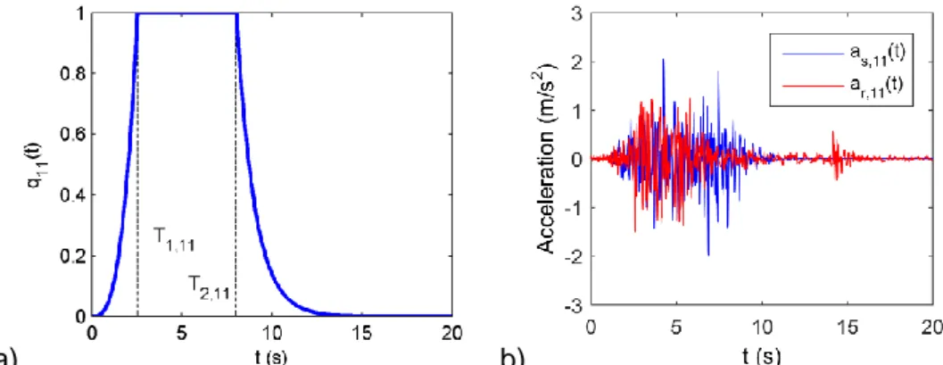
modulation functions, e.g. [29], may be considered. 133 134 𝑞𝑖(𝑡) = { ( 𝑡𝑇 1,𝑖) 3 0 ≤ 𝑡 ≤ 𝑇1,𝑖 1.0 𝑇1,𝑖< 𝑡 ≤ 𝑇2,𝑖 𝑒−(𝑡−𝑇2,𝑖) 𝑇 2,𝑖< 𝑡 ≤ 𝑡𝑑,𝑖 135 𝑖 = {1, … , 𝑁𝑟} (3) 136 137
where T1,i and T2,i are the times defining the plateau of this modulation function and td,i is the 138
total duration of the i-th acceleration record. Here, T1,i and T2,i are set equal to the times of
139
observation of the 5 % and 95 % of the Arias intensity in the original acceleration record. The 140
Arias intensity (Ir,i) of the i-th acceleration record is given by Equation 4.
141 142 𝐼𝑟,𝑖 =2𝑔𝜋 ∫ 𝛼𝑟,𝑖2(𝑡)𝑑𝑡, 𝑖 = {1, … , 𝑁 𝑟} 𝑡𝑑,𝑖 0 (4) 143 144
T1,i and T2,i are computed with Equations 5 and 6. As an example, Figure 1a shows the
145
modulation function used for the synthetic ground motions based on real record No. 11. 146 147 𝜋 2𝑔∫ 𝛼𝑟,𝑖2(𝑡)𝑑𝑡 = 0.05 ∙ 𝑇1,𝑖 0 𝐼𝑟,𝑖 𝑖 = {1, … , 𝑁𝑟} (5) 148 149 𝜋 2𝑔∫ 𝛼𝑟,𝑖2(𝑡)𝑑𝑡 = 0.95 ∙ 𝑇2,𝑖 0 𝐼𝑟,𝑖 𝑖 = {1, … , 𝑁𝑟} (6) 150 151
7
a) b)
152
Figure 1 a) Modulation function b) synthetic accelerogram and its original acceleration 153
record 154
155
The j-th realization of an unadjusted synthetic accelerogram (𝛼𝑠0,𝑖𝑗(𝑡)) based on the i-156
th acceleration record is given by Equation 7. 157 158 𝛼𝑠0,𝑖𝑗(𝑡) = 𝑞𝑖(𝑡) ∙ ∑ (𝐴𝑟,𝑖𝑚∙ 𝑠𝑖𝑛(𝜔𝑚+ 𝜑𝑠,𝑖𝑗𝑚)) 𝑛 𝑚=1 159 𝑖 = {1, … , 𝑁𝑟}, 𝑗 = {1, … , 𝑁𝑠} 160 (7) 161 162
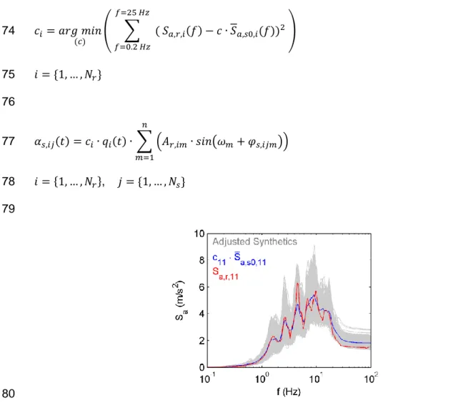
Subsequently, the synthetic ground motions generated based on an acceleration 163
record are all scaled with the same scaling factor (ci), which minimizes the sum of the squares
164
of the differences between the acceleration response spectrum of the acceleration record for 165
5 % damping (Sa,r,i(f)) and the median spectrum for 5 % damping of the scaled synthetic ground
166
motions (𝑐 ∙ 𝑆𝑎,𝑠0,𝑖(𝑓)) over the frequencies between 0.2 and 25 Hz (Equation 8). The adjusted
167
synthetic ground motions (𝛼𝑠,𝑖𝑗(𝑡)) are given by Equation 9. As an example, Figure 1b shows
168
record No. 11 and one of its spectrally equivalent synthetic accelerograms. Figure 2 shows 169
the acceleration response spectrum of ground motion record No. 11, the spectra of all 170
synthetic ground motions generated based on this record and the median spectrum of the 171
synthetics (𝑐11∙ 𝑆𝑎,𝑠0,11(𝑓)). 172
8 𝑐𝑖 = 𝑎𝑟𝑔 𝑚𝑖𝑛 (𝑐) ( ∑ ( 𝑆𝑎,𝑟,𝑖(𝑓) − 𝑐 ∙ 𝑆𝑎,𝑠0,𝑖(𝑓)) 2 𝑓=25 𝐻𝑧 𝑓=0.2 𝐻𝑧 ) 174 𝑖 = {1, … , 𝑁𝑟} (8) 175 176 𝛼𝑠,𝑖𝑗(𝑡) = 𝑐𝑖∙ 𝑞𝑖(𝑡) ∙ ∑ (𝐴𝑟,𝑖𝑚∙ 𝑠𝑖𝑛(𝜔𝑚+ 𝜑𝑠,𝑖𝑗𝑚)) 𝑛 𝑚=1 177 𝑖 = {1, … , 𝑁𝑟}, 𝑗 = {1, … , 𝑁𝑠} (9) 178 179 180
Figure 2 Acceleration response spectra for 5 % damping of the adjusted synthetic 181
ground motions and their original ground motion 182
183 184
Based on Nr = 96 original acceleration records, a total of Nr×Ns = 48000 “spectrally
185
equivalent” synthetic accelerograms are generated (Ns = 500 based on every acceleration
186
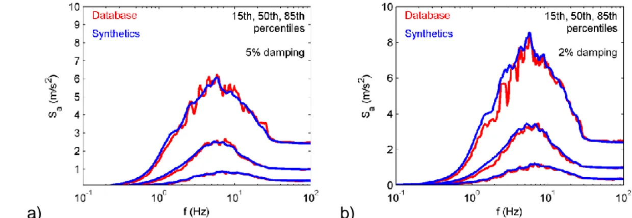
record) in order to be used in the analytical seismic fragility curve estimation. Figure 3a shows 187
the 15th, 50th and 85th percentiles of the acceleration response spectra for 5 % damping of the 188
ground motion records in the data set, and the corresponding percentiles of the spectra based 189
on the synthetic ground motions. The percentiles of the spectral values of the synthetic ground 190
motions match well that of the acceleration records and we consider that the ground motion 191
variability of the synthetics reproduces the variability in the original ground motion data set. 192
We observe in Figure 3b that the percentiles of the acceleration response spectra of the 193
synthetic ground motions for 2 % damping also match well the percentiles of the response 194
9
spectra of the acceleration records. Therefore, we consider that the adjustment technique is 195
quasi-independent of the damping value in the computation of the response spectra. 196
197
a) b)
198
Figure 3 Percentiles of the acceleration response spectra for a) 5 % and b) 2 % damping 199
of the synthetic accelerograms and the ground motions in the original data set 200
201
3 FRAGILITY CURVE CONSTRUCTION 202
3.1 Structural Model 203
For the illustrative application of this framework and for verification of the PMA-based 204
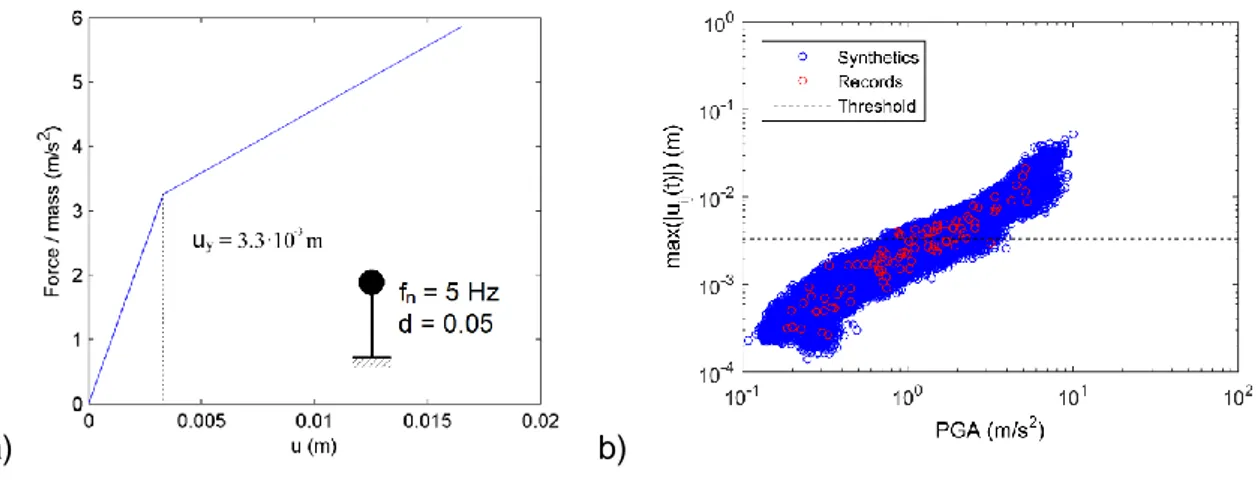
methodology an inelastic single degree of freedom structure is employed. Its frequency is 5 205
Hz, it has a damping ratio of 5 % and yield displacement (uy) of 3.3·10-3 m. Its post-yield 206
stiffness, defining kinematic hardening, is equal to the 20 % of its elastic stiffness (Figure 4a). 207
The response of the structure is computed by solving Equation 10 with the central difference 208 method. 209 210 𝑚𝑢̈𝑖𝑗(𝑡) + 𝑐𝑢̇𝑖𝑗(𝑡) + 𝑓𝑖𝑗(𝑡) = −𝑚𝛼𝑠,𝑖𝑗(𝑡) (10) 211 212
where m is the mass of the oscillator, 𝑢̈𝑖𝑗(𝑡) and 𝑢̇𝑖𝑗(𝑡) are the relative acceleration and velocity 213
of the mass, respectively, and 𝑓𝑖𝑗(𝑡) is the nonlinear resisting force. 214
10
a) b)
216 217
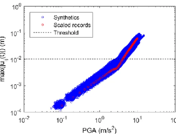
Figure 4 a) Backbone curve of the inelastic oscillator b) maximum oscillator 218
displacement (max(|uij(t)|)) observations as a function of the PGA
219 220
Figure 4b shows the maximum response of the inelastic oscillator under excitation with 221
the acceleration records and the generated synthetic ground motions. We observe that, in this 222
case, the responses under the synthetic ground motions are spread over an area between 223
and around the responses computed with the ground motion records. These data are used in 224
the different approaches here for deriving fragility curves. 225
3.2 Empirical Non-Parametric Fragility Curves Based On MC Simulations and IM 226
Clustering 227
The class of non-parametric fragility curves constructed here is based on MC 228
simulations and clustering of the Intensity Measure observations. In the illustrative example, 229
the maximum oscillator displacement is used as the EDP and the PGA is selected as IM for 230
simplicity while acknowledging that other IMs may be more efficient [30]. The total Intensity 231
Measure (IM) observations of all recorded and synthetic ground motions are classified to a 232
number of clusters with k-means clustering [23]. K-means clustering is an iterative optimization 233
procedure, which groups the IM observations in a selected number Nc of clusters. This
234
procedure also returns an IM value as the centroid of each cluster. The centroid of each cluster 235
is equal to the mean of the IM observations grouped in that cluster and the optimization 236
procedure consists in minimizing the sum of squares of its differences from the observations 237
11
in its cluster, i.e. the variance. Here, the IM observations are grouped into Nc = 20 clusters
238
using the function “kmeans” in MATLAB [31], while the effect of IM discretization is out of the 239
scope of this work. Subsequently, the point probabilities are classically computed at the IM 240
cluster centroids (Cl, l = {1,...,Nc}) as the ratio of the number of exceedances of the damage
241
state threshold, which are observed in the analyses corresponding to the IMs in a cluster, to 242
the number of total observations in the cluster. In this case, the damage state threshold is 243
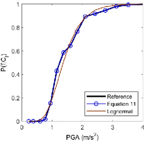
equal to the yield displacement (3.3·10-3 m) without loss of generality. Figure 5 shows the non-244
parametric fragility curve computed in this case with 48096 seismic response analyses using 245
all available recorded and synthetic accelerograms. Whenever the entirety of original and 246
synthetic ground motions is used, the empirical Monte-Carlo-based non-parametric fragility 247
curve will be called “reference”. The derivation of the other curves in Figure 5 follows. 248
249
250
Figure 5 Lognormal, reference and fragility curve according to Equation 11 251
252
3.3 New Formulation Of The Non-Parametric Fragility Curves 253
The proposed PMA methodology in this paper for optimized estimation of non-254
parametric fragility curves is based on Equation 11. This equation expresses the discrete 255
12
fragility curve P(f│Cl), which is defined at Nc cluster centroids (Cl), by means of the law of total
256 probability. 257 258 𝑃(𝑓|𝐶𝑙) =∑𝑁𝑟𝑖=1(𝑃(𝑓|𝐶𝑙∩ 𝑆𝑖)∙𝑃(𝐶𝑙|𝑆𝑖)∙𝑃(𝑆𝑖)) ∑𝑁𝑟𝑖=1(𝑃(𝐶𝑙|𝑆𝑖)∙𝑃(𝑆𝑖)) (11) 259 260
The conditional probability P(f|Cl∩Si) corresponds to the probability of exceeding the
261
damage state threshold at cluster centroid Cl under excitation with ground motions originating
262
from random process Si. This is practically the fragility curve estimated with the ground
263
motions originating from process Si. The conditional probability P(Cl|Si) is the probability of
264
sorting the IM observations, which correspond to the ground motions belonging to process Si,
265
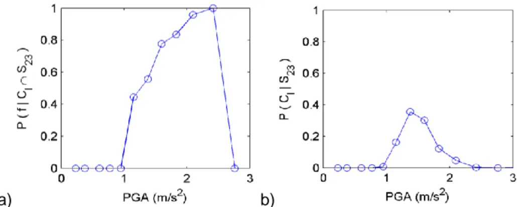
in the l-th cluster. As an example, Figures 6a and 6b show P(f|Cl∩S23) and P(Cl|S23),
266
respectively, which result from an empirical computation. Finally, the probability P(Si) equals
267
the fraction of the number of ground motions used, which belong to random process Si, to the
268
total number of ground motions used to estimate the fragility curve. If we generate an equal 269
number of synthetic ground motions for every one of Nr acceleration records, and all available
270
ground motions are used in the computation, then P(Si) = 1/Nr. This is the case in the validation
271
of the Equation 11 which is presented in Figure 5. We use 96x500 synthetic ground motions 272
generated by the random processes Si in addition to the 96 ground motions in the original data
273
set. Figure 5 shows that, as expected, the fragility curve defined by Equation 11 coincides with 274
the empirical fragility curve used as reference. 275
276 277
13
a) b)
278
Figure 6 a) Empirical probability of exceeding the damage state threshold (max(|uij(t)|)
279
= 3.3∙10-3 m) based on the synthetics generated based on the acceleration record S 23 at
280
the cluster centroids (Cl) b) probability of observing a PGA value in the synthetics
281
based on acceleration record S23
282 283
3.4 Lognormal Curve Adjusted To The Non-Parametric Curve 284
In order to observe potential differences between lognormal fragility curves and the non-285
parametric curves estimated with the different approaches herein, a Maximum Likelihood 286
Estimation of the lognormal cumulative distribution function is employed. The MLE of the 287
lognormal curve uses the point probabilities constituting the empirical fragility curve based on 288
the selected IM and corresponding EDP observations. The MLE is performed with Equations 289
12-15 and the estimated lognormal curve is given by Equation 16. 290 291 𝑃(𝑛𝑙, 𝑟𝑙, 𝐶𝑙) = 𝑛𝑙! 𝑟𝑙!(𝑛𝑙−𝑟𝑙)!∙ 𝑃(𝑓|𝐶𝑙) 𝑟𝑙∙ (1 − 𝑃(𝑓|𝐶 𝑙))𝑛𝑙−𝑟𝑙 (12) 292 293 𝐿 = ∏𝑁𝑐 𝑃(𝑛𝑙, 𝑟𝑙, 𝐶𝑙) 𝑙=1 (13) 294 295 ln (𝐿) = ∑ [𝑙𝑛 ( 𝑛𝑙! 𝑟𝑙!(𝑛𝑙−𝑟𝑙)!) + 𝑟𝑙∙ 𝑙𝑛𝛷 ( 𝑙𝑛(𝐶𝑙)−𝑙𝑛(A) 𝛽 ) + (𝑛𝑙− 𝑟𝑙) ∙ 𝑙𝑛 (1 − 𝛷 ( 𝑙𝑛(𝐶𝑙)−𝑙𝑛(A) 𝛽 ))] 𝑁𝑐 𝑙=1 (14) 296 297 {𝐴̅, 𝛽̅} = 𝑎𝑟𝑔 𝑚𝑎𝑥 (𝐴,𝛽) (𝑙𝑛 (𝐿)) (15) 298 299
14
𝑃(𝑓|𝐼𝑀) = 𝛷 (𝑙𝑛𝐼𝑀−𝑙𝑛𝐴̅𝛽̅ ) (16)
300 301
Where nl is the number of EDP observations corresponding to the IM observations in the l-th
302
cluster, rl is the number of EDP observations, which correspond to the IM observations in the
303
l-th cluster, that exceed the damage state threshold, Cl the IM centroid of the l-th cluster, P(f|Cl)
304
the empirical fraction of EDP observations exceeding the damage state threshold in the l-th 305
cluster, P(nl,rl,Cl) the binomial distribution, L the likelihood function, Φ the standard normal
306
cumulative distribution function, A and β the median and the dispersion of the lognormal 307
distribution, respectively, 𝐴̅ and 𝛽̅ their estimations, P(f|IM) the probability of exceeding the 308
damage state threshold given the IM. The difference with the curve fitting by Baker [4] is that 309
the fractions of damage state threshold exceedances at the cluster IM centroids are used 310
instead of the fractions at the IMs of EDP stripes. Figure 5 includes a lognormal curve 311
computed with this approach using the point probabilities, which constitute the reference 312
fragility curve. 313
4 OPTIMIZATION WITH PARAMETRIC MODELS AVERAGING 314
In order to illustrate the optimization of the non-parametric clustering fragility curve 315
estimation, we are employing five approaches: (i) MC optimized, (ii) lognormal un-316
optimized, (iii) lognormal optimized, (iv) PMA – Model 1 and PMA – Model 2, and (v) reference. 317
The reference curve has already been described and used in the validation of Equation 11. 318
PMA – Model 1 and PMA – Model 2 are the two forms of the optimized approach which are 319
described in Sections 4.1-4.2. 320
In the MC un-optimized approach, the number of seismic response analyses is firstly 321
selected. Subsequently, an equal number of IM observations are selected from every cluster, 322
equal to the number of total analyses divided by the number of clusters (rounded down to the 323
closest integer). If there are less IM observations in some clusters than required, we select 324
those available and we select the rest by selecting an even number of observations from the 325
15
rest clusters and so on. After determining the number of IM observations per cluster that will 326
be selected, the actual selection of the IM observations is made. This selection is based on 327
the results of k-means clustering of the IM observations based on all synthetic and recorded 328
accelerograms. K-means returns for every IM observation the index of the cluster to which the 329
observation is sorted. Based on the returned indices, lists of the IM observations per cluster 330
are made and the required observations per cluster are randomly selected from the 331
corresponding lists. Subsequently, the seismic ground motions, which correspond to the 332
selected IM observations, are used as excitations in dynamic time-history analyses of the 333
oscillator in order to compute EDP observations. In the MC un-optimized approach, as in the 334
reference, the probability of exceeding the damage state threshold is estimated empirically at 335
the l-th cluster centroid as the observed fraction of EDP observations exceeding the damage 336
state threshold to the total number of EDP observations corresponding to the IM observations 337
in the cluster. The lognormal curve derived using the data used in the MC un-optimized 338
approach will be called lognormal un-optimized. 339
The optimized PMA approach is based on Equation 11 and follows the procedure of the 340
MC un-optimized approach with three modifications. First, the conditional probability P(Cl|Si)
341
is not estimated with the selected IM observations, but with a very large number of IM 342
observations in order to obtain a very precise estimation. Here, each P(Cl|Si) distribution is
343
empirically estimated with all available 501 IM observations; 500 observations corresponding 344
to the synthetics and 1 to the original acceleration record. Practically, this means that the 345
estimation of P(Cl|Si) in the optimized approach and in the computation for the reference
346
fragility curve are identical. It is worth noting that the estimation of P(Cl|Si) does not require
347
any seismic response analyses, but it requires only IM observations based on synthetic ground 348
motions, which has a small computational cost. Second, IM observations (and the 349
corresponding seismic ground motions used to compute EDP observations through seismic 350
response analyses) are selected only if they are sorted in a cluster ki where P(Cl|Si) reaches
351
its maximum. This is one of the key elements of the optimization process. In order to do so, 352
the IM observations sorted in clusters other than the cluster, where P(Cl|Si) of their process of
16
origin is maximized, are expunged from the lists of IM observations per cluster, from which IM 354
observations are randomly drawn. The third and most important modification concerns the 355
conditional probability of exceeding the damage state threshold in the case of each process 356
(P(f|Cl∩Si)). Instead of the empirical estimation of P(f|Cl∩Si), the optimized approach employs
357
two alternative parametric models. The first model (parametric model 1) assumes that 358
P(f|Cl∩Si) remains constant as a function of the IM, and that it is equal to P(f|Cki∩Si). The
359
second model (parametric model 2) uses a lognormal curve for P(f|Cl∩Si). In the following, the
360
parametric models 1 and 2 are analyzed. 361
4.1 Parametric Model 1 362
The first model for P(f|Cl∩Si) is defined by a single parameter for every process. When
363
using this model, the optimized approach will be called PMA – Model 1. This one parameter 364
is taken equal to the empirical estimation of the probability of exceeding the damage state 365
threshold at the ki-th IM cluster centroid, where 𝑃(𝐶𝑙|𝑆𝑖) obtains its maximum value (Equation
366
17). The one-parameter models are defined by Equation 18 and model the probability of 367
exceeding the damage state threshold (𝑃𝑓𝑖) per process as constant throughout all cluster IM 368 centroids. 369 370 𝑘𝑖 = 𝑎𝑟𝑔 𝑚𝑎𝑥 (𝑙) 𝑃(𝐶𝑙|𝑆𝑖) 371 𝑖 = {1, … , 𝑁𝑟 = 96}, 𝑙 = {1, … , 𝑁𝑐 = 20} (17) 372 373 𝑃𝑓𝑖 = 𝑃(𝑓|𝐶𝑙∩ 𝑆𝑖) = 𝑃(𝑓|𝐶𝑘𝑖∩ 𝑆𝑖) 374 𝑖 = {1, … , 𝑁𝑟 = 96}, 𝑙 = {1, … , 𝑁𝑐 = 20} (18) 375 376
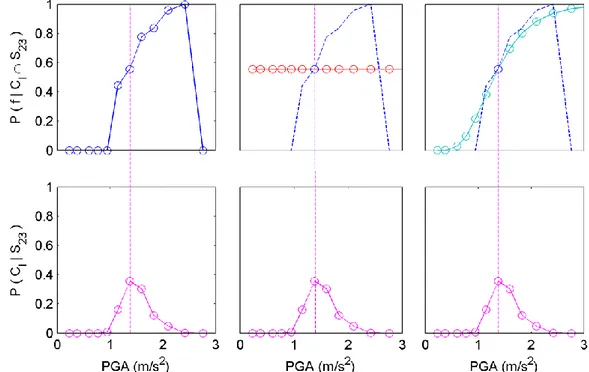
As an example, Figure 7 (top left) shows the empirical conditional probability 377
𝑃(𝑓|𝐶𝑘23∩ 𝑆23) estimated with the observations corresponding to the ground motions based
378
on the 23rd accelerogram record. Moreover, Figure 7 (top middle) shows the corresponding 379
17
model used in the optimized approach, which assumes a constant probability (red curve), 380
which is estimated at the cluster IM centroid for which 𝑃(𝐶𝑙|𝑆23) is maximized (Figure 7 381
bottom). When employing parametric model 1, an error is introduced with respect to P(f|Cl∩Si).
382
In specific, P(f|Cl∩Si) is under- and overestimated at IM cluster centroids where Cl > Ck and Cl 383
< Ck, respectively. The extent to which P(f|Cl∩Si) is under- or overestimated varies, and
384
generally increases with the distance between Cl and Ck. However, the introduced error is 385
mitigated by the fact that Equation 11 computes the product P(f|Cl∩Si)·P(Cl|Si). The farther Cl 386
is found from Ck, the smallest the introduced error, because P(Cl|Si) diminishes with the
387
distance from Ck (e.g. Figure 7 bottom). Moreover, the fact that P(f|Cl∩Si) is simultaneously
388
under- and overestimated (e.g. Figure 7 middle) at Cl > Ck and Cl < Ck, respectively, also 389
mitigates the global error in the estimation of the fragility curve, as the underestimation on one 390
side balances to some extent the overestimation on the other. 391
392
393
Figure 7 Top left: Empirical fragility curve based on the ground motions originating 394
from acceleration record 23. Top middle: parametric model 1 (constant probability of 395
damage state threshold exceedance). Top right: parametric model 2 (lognormal model) 396
Bottom: conditional probability P(Cl|S23).
397 398
18 4.2 Parametric Model 2
399
The lognormal curve is used as the second alternative parametric model for P(f|Cl∩Si)
400
for every process. This form of the optimized approach will be called PMA – Model 2. In order 401
to define this model for every process, two parameters are required: the dispersion and the 402
median of the lognormal curve. These two parameters could be computed, if two or more point 403
probabilities were available, to which the lognormal curve might be fitted. Since the optimized 404
approach selects only IMs (and corresponding accelerograms) in cluster ki, where P(Cl|Si) is
405
maximized, and computes the corresponding EDPs and 𝑃(𝑓|𝐶𝑘𝑖∩ 𝑆𝑖), the only available point
406
probability is (𝐶𝑘𝑖, 𝑃(𝑓|𝐶𝑘𝑖∩ 𝑆𝑖)). Therefore, we assume that the dispersion of the lognormal
407
curve for every process (βi) is equal to the dispersion of the lognormal fragility curve (𝛽̅, which 408
will be referred to as β for simplicity), which is derived with Equations 12-16 using the data 409
selected according to the optimized approach. This curve will be called lognormal optimized 410
(there is no actual optimization here, this is simply part of the naming scheme). This allows us 411
to compute the median of the curve for every process (Ai) with Equation 19. Based on Ai and
412
βi, the parametric model for every process is subsequently defined with Equation 20.
413 414 𝐴𝑖 = 𝑒𝑥𝑝 (ln(𝐶𝑘𝑖) − 𝛽𝑖∙ 𝛷−1(𝑃(𝑓|𝐶𝑘𝑖∩ 𝑆𝑖))) 415 𝛽𝑖 = 𝛽 (19) 416 417 𝑃(𝑓|𝐶𝑙∩ 𝑆𝑖) = 𝛷 (ln(𝐶𝑙)−ln(𝐴𝛽 𝑖) 𝑖 ) (20) 418 419
As an example, Figure 7 (top right) shows P(f|Cl∩S23) as estimated with the lognormal
420
parametric model (cyan curve). In this case, the model approximates well the empirical 421
estimation of the probability of exceeding the damage state threshold. This figure illustrates 422
that the largest differences between the probabilities given by the model and the empirical 423
estimation are observed where P(Cl|Si) is close to zero. However, the empirical probabilities
19
P(Cl|Si) are equal to zero at the IM centroids of clusters without any IM observations.
425
Therefore, at such cluster IM centroids, the product P(f|Cl∩Si)·P(Cl|Si) in Equation 11 is always
426
zero, which means that no error is introduced at these clusters due to the use of a parametric 427
model for P(f|Cl∩Si). As shown in the following, parametric model 2 is particularly necessary
428
when the dispersion of the lognormal optimized fragility curve is small (approximately for β < 429
0.3). In such cases, we consider justified to impose a common dispersion on all the parametric 430
models corresponding to the processes Si. 431
5 APPLICATION OF THE METHODOLOGY 432
In order to offer insight to the wider field of application of the developed methodology, 433
which is essentially a MC procedure, we use it to compute the fragility curves in three cases: 434
(i) inelastic oscillator without structural uncertainties and ground motions selected at random 435
form the data set of all recorded and synthetic ground motions, (ii) inelastic oscillator without 436
structural uncertainties and ground motions resulting from scaling of a single recorded 437
accelerogram, (iii) inelastic oscillator with structural uncertainties. Based on the results of 438
these three cases, we make our recommendations for practice. In the third case, the fragility 439
curves are derived using as IM the PGA and the spectral acceleration at the frequency of the 440
oscillator (Sa(5 Hz)). To evaluate the effectiveness of the optimized procedures, we are 441
comparing the estimated fragility curves with the reference curve and the 95 % CI according 442
to the different approaches. The CI are computed based on bootstrap resampling [32] with a 443
different set of 500 curves for each case. 444
5.1 Structural Model Without Uncertainties And Data Set Of Acceleration Records 445
The developed PMA-based optimization is firstly applied it in the case of the inelastic 446
oscillator employed previously in the description of the methodology (Figure 4a). The ground 447
motion data set used consists of the 96 recorded accelerograms and the 48,000 448
corresponding synthetic ground motions generated with the described procedure in section 2. 449
20
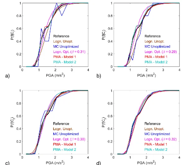
The fragility curves are computed as a function of the PGA, for a damage state threshold 450
defined by a maximum oscillator displacement of 3.3·10-3 m, and according to the different 451
approaches are shown in Figure 8 in the case of 100, 200, 500, and 10,000 analyses, 452
respectively. The curves MC un-optimized and lognormal un-optimized are computed based 453
on the same set of seismic response analyses, which is different from the set of analyses used 454
for the optimized non-parametric curves. Every set of seismic response analyses is performed 455
using a different and randomly selected set of ground motions according to the optimized or 456
un-optimized approaches. Additionally, the reference non-parametric fragility curve, which is 457
estimated based on 48096 analyses with all recorded and synthetic accelerograms, is included 458
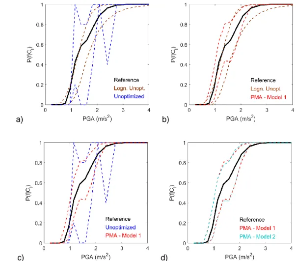
in the figures in order to observe any potential statistical error or bias in the evaluated curves. 459 460 a) b) 461 c) d) 462
Figure 8 Fragility curves for maximum oscillator displacement (max(|uij(t)|)) threshold
463
of 3.3·10-3 m evaluated without structural uncertainties and with the enriched ground
21
motion data set based all considered records and based on a) 100 b) 200 c) 500 and d) 465
10,000 analyses, and the reference non-parametric fragility curve 466
467
In the case of 100, 200 and 500 seismic response analyses (Figure 8a-c), the 468
differences between the reference and the rest fragility curves is primarily due to error of 469
estimation. However, in the case of 10,000 analyses, the difference is rather due to a bias in 470
the computation, given that the fragility curves are evaluated with a very large number of 471
analyses. As far as the MC un-optimized and PMA curves are concerned, they practically 472
converge with the reference curve as the number of analyses increases, which means that no 473
bias is introduced due to the assumptions in this case. In Figure 8d, we observe differences 474
between the reference and the lognormal un-optimized curve based on 10,000 analyses. 475
Given the number of analyses, we consider that the lognormal curve is biased. More important 476
differences between lognormal and non-parametric curves may be observed, when –among 477
other reasons– the studied structures are more complex than a single-degree-of-freedom 478
oscillator, as in [18]. As a measure of the estimation error, the 95 % CI of the fragility curve 479
based on 100 analyses and according to the different approaches are shown in Figure 9. As 480
expected, the MC un-optimized approach gives a poor estimation (Figure 9a) due to the small 481
amount of data and the lognormal un-optimized is more effective. The CI of the curves 482
according to the lognormal un-optimized and the PMA – Model 1 approaches appear to be 483
equivalent (Figure 9b). However, the median lognormal un-optimized curve may converge 484
towards a biased estimation (e.g. Figure 8). Therefore, its confidence interval is not 485
necessarily representative of the goodness of the estimation. This is a weakness of the 486
parametric models and it is beforehand unknown whether there is bias in the fragility curve in 487
complex cases. We observe that the PMA – Model 1 approach results in CI which are 488
significantly smaller than the CI according to the MC un-optimized approach (Figure 9c). 489
According to the curves in Figure 9d, we conclude that the two forms of the PMA optimization 490
are equally effective in this case. 491
22
a) b)
493
c) d)
494
Figure 9 95 % confidence intervals of fragility curves for maximum oscillator 495
displacement (max(|uij(t)|)) threshold of 3.3·10-3 m evaluated without structural
496
uncertainties and with the enriched ground motion data set based all considered 497
records and based on 100 analyses, and the reference non-parametric fragility curve 498
499
5.2 Structural Model Without Uncertainties And Data Set Of A Multiply Scaled 500
Acceleration Record 501
Here we study a case with limited ground motion variability in order to demonstrate that 502
the applicability of the developed procedures for non-parametric fragility curve estimation 503
depends on the dispersion of the lognormal optimized curve, which is fitted to the data in an 504
intermediate step of the computation. In this case, the synthetic ground motions are generated 505
based on artificial accelerograms, which result from scaling multiple times (100 in this case) a 506
randomly selected acceleration record from the 96 original real records. Based on each 507
artificial accelerogram, 500 synthetic ground motions are generated with the procedure in 508
23
Section 2.2. Again, the oscillator in Figure 4a is employed. The maximum oscillator 509
displacements as a function of the PGA based on all synthetic and artificial records, which are 510
used for the reference non-parametric curve for this case, are shown in Figure 10. 511
512
513
Figure 10 Maximum oscillator displacement (max(|uij(t)|)) as a function of PGA
514
computed without structural uncertainties and with the enriched ground motion data 515
set based on scaling of a single randomly selected recorded accelerogram 516
517
The fragility curves for a damage state threshold defined by a maximum oscillator 518
displacement of 1.0·10-2 m according to the different considered approaches using 100, 200, 519
500, and 10,000 seismic response analyses are shown in Figure 11. In this case, all fragility 520
curves converge to the reference with the exception of the PMA – Model 1 curve, which is 521
based on the optimization assuming models of constant P(f|Cl∩Si) per process. It is concluded
522
that PMA model 1 produces a biased curve contrary to PMA model 2 (Figure 11d). 523
Nevertheless, PMA model 2 may also result in bias in other cases (not shown here), when the 524
dispersion of the unoptimized lognormal curve is very small (β < 0.1). Indeed, in such cases, 525
the reference fragility curve tends towards a step function, which cannot be approximated by 526
the PMA-based procedures presented here unless a finer IM discretization is considered. It 527
should also be taken into account that the observed difference between the reference curve 528
and the curves according to the different approaches in the case of 100 and 200 seismic 529
response analyses is principally an estimation error due to the limited number of seismic 530
response analyses used. 531
24 532 a) b) 533 c) d) 534
Figure 11 Fragility curves for maximum oscillator displacement (max(|uij(t)|)) threshold
535
of 1.0·10-2 m evaluated without structural uncertainties and with the enriched ground
536
motion data set based on scaling of acceleration record 27 and based on a) 100 b) 200 537
c) 500 and d) 10,000 analyses, and the reference non-parametric fragility curve 538
539
Figure 12 includes the 95 % CI of the fragility curves based on 100 seismic response 540
analyses. Also in this case, the lognormal optimized is more effective than the MC un-541
optimized. The CI of the lognormal un-optimized and PMA – Model 2 curves indicate that both 542
approaches are effective in this case, with PMA – Model 2 being slightly better. Once more, 543
the estimation error according to the PMA – Model 2 approach is significantly less than the 544
error in the case of the MC un-optimized computation with 100 analyses. Contrary to the CI of 545
PMA – Model 1 curve, the CI of the PMA – model 2 curve envelopes the reference and 546
indicates that this is the preferable approach in this case. 547
25
a) b)
549
c) d)
550
Figure 12 95 % confidence intervals of fragility curves for maximum oscillator 551
displacement (max(|uij(t)|)) threshold of 1.0·10-2 m evaluated without structural
552
uncertainties and with the enriched ground motion data set based on scaling of 553
acceleration record 27 and based on 100 analyses, and the reference non-parametric 554
fragility curve 555
556
5.3 Structural Model With Uncertainties And Data Set Of Acceleration Records 557
The developed optimization procedure is also applied in the case of uncertain structural 558
parameters. In specific, the oscillator in Figure 4a is employed and uncertainty is introduced 559
by considering the elastic frequency and the yield displacement of the oscillator as random 560
parameters with a coefficient of variation of 0.2. To do so, in every simulation, i.e. seismic 561
response analysis, the elastic frequency (5.0 Hz) and the yield displacement (3.3·10-3 m) are 562
multiplied with random independent values sampled from two identical normal distributions 563
with mean and standard deviation equal to 1.0 and 0.2, respectively. Such pairs of random 564
values are sampled with Latin Hypercube Sampling for all 96 records and 48000 synthetic 565
26
ground motions in the data set. Figure 13 shows the damage state threshold and the computed 566
EDPs (max(|uij(t)|)) as a function of Sa(5 Hz) and PGA as IM, respectively. 567
568
a) b)
569
Figure 13 Maximum oscillator displacement (max(|uij(t)|)) as a function of a) the spectral
570
acceleration at 5 Hz and b) the PGA in the case of the oscillator with frequency and 571
yield displacement uncertainty 572
573
The fragility curves for a damage state threshold of 3.3·10-3 m maximum oscillator 574
displacement as a function of Sa(5 Hz) and PGA are shown in Figure 14 and 15. As expected, 575
(i) the introduction of uncertainties leads to increase of the dispersion of the lognormal fragility 576
curves and (ii) the dispersion of the lognormal fragility curves is slightly larger when PGA is 577
considered as IM. The optimized fragility curves and un-optimized non-parametric fragility 578
curves converge with the reference fragility curves in both cases (Figures 14d, 15d) and 579
present small differences from the lognormal curves. It is worth noting that the lognormal 580
optimized curve has a dispersion of 0.48 and 0.52 when using as IM the Sa(5 Hz) and the 581
PGA, respectively. 582
27
a) b)
584
c) d)
585
Figure 14 Spectral acceleration (Sa(5 Hz))-based fragility curves for maximum oscillator
586
displacement (max(|uij(t)|)) threshold of 3.3·10-3 m evaluated with structural
587
uncertainties and with the enriched ground motion data set based all considered 588
records and based on a) 100 b) 200 c) 500 and d) 10,000 analyses, and the reference 589
non-parametric fragility curve 590
28
a) b)
592
c) d)
593
Figure 15 PGA-based fragility curves for maximum oscillator displacement (max(|uij(t)|))
594
threshold of 3.3·10-3 m evaluated with structural uncertainties and with the enriched
595
ground motion data set based all considered records and based on a) 100 b) 200 c) 500 596
and d) 10,000 analyses, and the reference non-parametric fragility curve 597
598
6 CONCLUSION 599
Here, we present a procedure for optimized derivation of non-parametric fragility curves 600
using synthetic accelerograms. The fragility curves given by the presented procedure are 601
intended for use for a specific structure rather than for a class of structures. A simple synthetic 602
accelerogram generator is used, which reproduces the ground motion variability observed in 603
a data set of ground motion records. However, the presented procedure is more general since 604
it can use synthetic ground motions from other generators as long as they define random 605
processes similar to those defined here. Also, note that the presented procedure is 606
29
independent of the selected IM. The optimization relies on the fact that the generated synthetic 607
signals are realizations of a series of stochastic processes, each of which is based –in this 608
work– on an acceleration record in the original data set. Using the EDP observations based 609
on the synthetic ground motions, a parametric fragility curve is estimated for each process. 610
Two alternative parametric models per process are proposed: a lognormal model and a model 611
of constant probability of exceeding the damage state threshold. Based on the estimated 612
models for all processes considered, a non-parametric fragility curve is estimated based on 613
PMA, which computes the weighted average of the parametric models according to the law of 614
total probability. 615
For the illustrative cases herein, synthetic ground motions are generated with a “simple” 616
generator, which uses an original set of acceleration records. The generator produces 617
synthetic ground motions with acceleration response spectra, whose 15th, 50th and 85th 618
percentiles match well the corresponding percentiles of the spectral values of the ground 619
motions in the original data set. All recorded and synthetic accelerograms are used as 620
excitations of an inelastic single degree of freedom oscillator in order to obtain EDP 621
observations as a function of the IM and estimate a reference fragility curve. The entirety of 622
the IM observations of the recorded and synthetic ground motions is classified to clusters with 623
k-means clustering. The number of clusters is selected based on engineering judgment, since 624
the effect of the number of clusters is not studied here, and may nevertheless be a factor 625
limiting the applicability of this methodology in some cases. Subsequently, the probability of 626
exceeding the damage state threshold is estimated empirically at the cluster IM centroids 627
using the EDP observations corresponding to the IM observations in each cluster. The result 628
is the MC-based empirical non-parametric fragility curve, which is used as reference, as it is 629
considered the best estimation possible based on the IM clustering approach and the available 630
data. In the MC un-optimized approach, the same procedure is followed, but instead of using 631
all data, an as constant as possible number of IM observations per cluster is selected so that 632
the total number of analyses is in accordance with the available computational time. 633
30
The PMA optimized approach builds upon the MC un-optimized estimation by introducing 634
an additional IM observation selection criterion. The IM observations in every cluster eligible 635
for selection are those found in clusters with maximum probability of observation given the 636
process, which generated the corresponding synthetic ground motions. Based on the EDP 637
observations, which correspond to the selected IM observations, the probabilities of exceeding 638
the damage state threshold at the IM cluster centroids are empirically estimated. These 639
probabilities are used to define the parametric fragility curve, i.e. the parametric mode, which 640
is related to each random process. Subsequently, the parametric models are averaged with 641
the probabilities of occurrence of each random process in the clusters which are estimated 642
with a very large number of synthetic ground motions, with practically no computational cost, 643
since it requires no seismic response analyses. As in [18] or [21], we observe that non-644
parametric curves based on the proposed procedures may present differences from lognormal 645
curves based on the same data. Here, the smallest differences between lognormal un-646
optimized and non-parametric fragility curves are observed when the dispersion of the 647
lognormal curves are either very small (e.g. < 0.1) or considerable (e.g. > 0.5). As far as the 648
uncertainty of the estimated non-parametric curve is concerned, we employ non-parametric 649
bootstrap resampling to estimate the 95 % CI of the fragility curves. Moreover, the 95 % CI of 650
the PMA curve is reduced with respect to the CI of the MC un-optimized curve for the same 651
number of seismic response analyses in all cases in the study. In conclusion, the developed 652
methodology is an efficient and useful procedure for fragility curve estimation and has wider 653
applicability than a parametric model (e.g. the lognormal), which may lead to biased 654
estimations. 655
Our recommendations are summarized in Table 1. The criteria that guide us are two: the 656
dispersion of the lognormal optimized curve fitted to the selected data and the discretization 657
of the IM observations, i.e. the number of clusters. When applying the proposed procedure, 658
estimating a fragility curve while using a very coarse IM discretization can be considered 659
equivalent to the estimation of a fragility curve with a very small dispersion. In the area of 100 660
or less analyses, use of a typical un-optimized lognormal fragility curve is recommended. If 661
31
the resources for 10,000 or more analyses are available, the MC un-optimized approach can 662
be used. In the area between 100 and 10,000 analyses, which is of practical interest, we 663
suggest either a parametric curve, or a non-parametric optimized fragility curve computation 664
with one of the two proposed alternatives. In this area, the dispersion of the optimized 665
lognormal curve fitted to the selected data dictates the optimal approach. In the case of a large 666
dispersion (0.3 ≤ β), the optimization with the constant probability of damage threshold 667
exceedance per process is sufficient, while in the case of a limited dispersion (0.1 ≤ β < 0.3), 668
the optimization with the lognormal model per process is recommended. When PMA – Model 669
1 and 2 use a large number of seismic response analyses and give drastically different results 670
(as in the case with an original data set consisting of ground motions resulting from scaling a 671
single acceleration record), PMA – Model 2 should be preferred, unless the dispersion of the 672
associated optimized lognormal curve is very small (β < 0.1). In such cases, the presented 673
PMA approaches are not efficient and a lognormal model for the fragility curve is 674
recommended. 675
676
Table 1 Recommended type of fragility curve based on the number of seismic analyses 677
(N) and the dispersion of the lognormal (un-optimized) curve fitted to the empirical non-678 parametric curve (β) 679 680 β < 0.1 0.1 ≤ β < 0.3 0.3 ≤ β N < 100 Un-optimized Lognormal Un-optimized Lognormal Un-optimized Lognormal 100 ≤ N < 10,000 Un-optimized
Lognormal PMA – Model 2 PMA – Model 1 10,000 ≤ N MC Un-optimized MC Un-optimized MC Un-optimized 681
Our procedure has also been applied in the case of a realistic finite element model of a low-682
rise reinforced concrete bare frame (modelling details may be found in [33]), not presented 683
here for the sake of brevity. The results lead to the same conclusions. Should one attempt to 684
apply the procedure herein in the case of complex structures, they will face a series of 685
challenges, which are, however, not specific to our methodology. A major concern would be 686
the selection of an efficient IM. IMs are considered efficient [34], when the seismic response 687
32
as a function of the IM has a low dispersion. However, scalar IMs are not efficient in every 688
case. For example, the spectral acceleration at the first eigenfrequency is a common scalar 689
IM, which is efficient in the case of structures, whose response is mostly affected by their first 690
mode. However, it is not efficient in the case of tall buildings [35]. In the case of structures with 691
multiple degrees of freedom the use of more adapted IMs, or even a vector of different IMs 692
[36] may be a solution. That said, further investigations should be made to see if the 693
procedures herein can be modified to use a vector IM. Although, the procedure herein is –in 694
principle– independent of the selected IM and the damage state, it should be adapted to more 695
severe damage states such as collapse. Indeed, the simulation of severe damage states may 696
be computationally demanding and may require to take into account P-delta effects [37], to 697
simulate brittle failure modes [38] and consider alternative IMs [39]. In addition, a validation of 698
our methodology with a very large number of seismic response analyses in the case of 699
complex structures has a prohibitive computational cost. To test the usefulness of our 700
procedure in the case of complex structures, fragility curves given by our procedure based on 701
a reasonable number of seismic response analyses (e.g. a few hundred) could be compared 702
with curves given by other procedures, which reduce the computational cost. Such procedures 703
may rely, amongst others, on metamodeling strategies based on neural networks [40], or 704
support vector machines [41]. Finally, further studies of the developed procedure using 705
realistic structural models and fragility curves conditioned on failure, instead of curves 706
conditioned on an engineering demand parameter threshold, should provide additional 707
insights. 708
ACKNOWLEDGMENTS 709
Funding: This work was supported by the research project SINAPS@ (ANR-11-RSNR-0022), 710
a project of the SEISM Institute (https://institut-seism.fr/) funded by The French National 711
Research Agency in the context of its program Investments for the Future. 712
33 REFERENCES
713
[1] Fragiadakis M, Vamvatsikos D, Karlaftis MG, Lagaros ND, Papadrakakis M. Seismic 714
assessment of structures and lifelines. J Sound Vib 2015;334:29–56. 715
doi:10.1016/j.jsv.2013.12.031. 716
[2] Yang TY, Moehle J, Stojadinovic B, Der Kiureghian A. Seismic Performance Evaluation 717
of Facilities: Methodology and Implementation. J Struct Eng 2009;135:1146–54. 718
doi:10.1061/(ASCE)0733-9445(2009)135:10(1146). 719
[3] FEMA. Seismic Performance Assessment of Buildings – Volume 1 – Methodology. 720
WAshington, DC: 2012. 721
[4] Baker JW. Efficient Analytical Fragility Function Fitting Using Dynamic Structural 722
Analysis. Earthq Spectra 2015;31:579–99. doi:10.1193/021113EQS025M. 723
[5] Silva V, Crowley H, Bazzurro P. Exploring Risk-Targeted Hazard Maps for Europe. 724
Earthq Spectra 2016;32:1165–86. doi:10.1193/112514EQS198M. 725
[6] Berge-Thierry C, Svay A, Laurendeau A, Chartier T, Perron V, Guyonnet-Benaize C, 726
et al. Toward an integrated seismic risk assessment for nuclear safety improving current 727
French methodologies through the SINAPS@ research project. Nucl Eng Des 2017;323:185– 728
201. doi:10.1016/j.nucengdes.2016.07.004. 729
[7] Tsionis G, Mignan D, Pinto A, Giardini D, European Commission, Joint Research 730
Centre. Harmonized approach to stress tests for critical infrastructures against natural 731
hazards. Luxembourg: Publications Office; 2016. 732
[8] Zhang J, Huo Y. Evaluating effectiveness and optimum design of isolation devices for 733
highway bridges using the fragility function method. Eng Struct 2009;31:1648–60. 734
doi:10.1016/j.engstruct.2009.02.017. 735
[9] Saha SK, Matsagar V, Chakraborty S. Uncertainty quantification and seismic fragility 736
of base-isolated liquid storage tanks using response surface models. Probabilistic Eng Mech 737
2016;43:20–35. doi:10.1016/j.probengmech.2015.10.008. 738
34
[10] Patil A, Jung S, Kwon O-S. Structural performance of a parked wind turbine tower 739
subjected to strong ground motions. Eng Struct 2016;120:92–102. 740
doi:10.1016/j.engstruct.2016.04.020. 741
[11] Gidaris I, Taflanidis AA, Mavroeidis GP. Kriging metamodeling in seismic risk 742
assessment based on stochastic ground motion models: Seismic Risk Assessment Through 743
Kriging Metamodeling. Earthq Eng Struct Dyn 2015;44:2377–99. doi:10.1002/eqe.2586. 744
[12] Parolai S, Haas M, Pittore M, Fleming K. Bridging the Gap Between Seismology and 745
Engineering: Towards Real-Time Damage Assessment. In: Pitilakis K, editor. Recent Adv. 746
Earthq. Eng. Eur., vol. 46, Cham: Springer International Publishing; 2018, p. 253–61. 747
doi:10.1007/978-3-319-75741-4_10. 748
[13] Quilligan A, O’Connor A, Pakrashi V. Fragility analysis of steel and concrete wind 749
turbine towers. Eng Struct 2012;36:270–82. doi:10.1016/j.engstruct.2011.12.013. 750
[14] D’Ayala D, Meslem A, Vamvatsikos D, Porter K, Rossetto T, Silva V. Guidelines for 751
Analytical Vulnerability Assessment - Low/Mid-Rise. GEM; 2015. 752
[15] Vamvatsikos D, Cornell CA. Incremental dynamic analysis. Earthq Eng Struct Dyn 753
2002;31:491–514. doi:10.1002/eqe.141. 754
[16] Jalayer F, Cornell CA. Alternative non-linear demand estimation methods for 755
probability-based seismic assessments. Earthq Eng Struct Dyn 2009;38:951–72. 756
doi:10.1002/eqe.876. 757
[17] Zentner I. A general framework for the estimation of analytical fragility functions based 758
on multivariate probability distributions. Struct Saf 2017;64:54–61. 759
doi:10.1016/j.strusafe.2016.09.003. 760
[18] Mai C, Konakli K, Sudret B. Seismic fragility curves for structures using non-parametric 761
representations. Front Struct Civ Eng 2017;11:169–86. doi:10.1007/s11709-017-0385-y. 762
[19] Noh HY, Lallemant D, Kiremidjian AS. Development of empirical and analytical fragility 763
functions using kernel smoothing methods: DEVELOPMENT OF FRAGILITY FUNCTIONS 764
USING KERNEL SMOOTHING METHODS. Earthq Eng Struct Dyn 2015;44:1163–80. 765
doi:10.1002/eqe.2505. 766