HAL Id: hal-01159641
https://hal.inria.fr/hal-01159641v2
Submitted on 25 Sep 2015
HAL is a multi-disciplinary open access
archive for the deposit and dissemination of
sci-entific research documents, whether they are
pub-lished or not. The documents may come from
L’archive ouverte pluridisciplinaire HAL, est
destinée au dépôt et à la diffusion de documents
scientifiques de niveau recherche, publiés ou non,
émanant des établissements d’enseignement et de
Binding Affinity Predictions
Simon Marillet, Pierre Boudinot, Frédéric Cazals
To cite this version:
Simon Marillet, Pierre Boudinot, Frédéric Cazals. High Resolution Crystal Structures Leverage
Pro-tein Binding Affinity Predictions. [Research Report] RR-8733, Inria. 2015. �hal-01159641v2�
0249-6399 ISRN INRIA/RR--8733--FR+ENG
RESEARCH
REPORT
N° 8733
September 2015Structures Leverage
Protein Binding Affinity
Predictions
RESEARCH CENTRE
SOPHIA ANTIPOLIS – MÉDITERRANÉE
2004 route des Lucioles - BP 93
Simon Marillet
∗and Pierre Boudinot
†and Frédéric Cazals
‡Project-Team Algorithms-Biology-Structure
Research Report n° 8733 — version 2 — initial version September 2015 — revised version Septembre 2015 — 42 pages
Abstract: Predicting protein binding affinities from structural data has remained elusive, a difficulty owing to the variety of protein binding modes. Using the structure-affinity-benchmark (SAB, 144 cases with bound/unbound crystal structures and experimental affinity measurements), prediction has been undertaken either by fitting a model using a handfull of pre-defined variables, or by training a complex model from a large pool of parameters (typically hundreds). The former route unnecessarily restricts the model space, while the latter is prone to overfitting.
We design models in a third tier, using twelve variables describing enthalpic and entropic variations upon binding, and a model selection procedure identifying the best sparse model built from a subset of these variables. Using these models, we report three main results. First, we present models yielding a marked improvement of affinity predictions. For the whole dataset, we present a model predicting Kd within one and two orders of magnitude for 48% and 79% of cases, respectively. These statistics jump to 62% and 89% respectively, for the subset of the SAB consisting of high resolution structures. Second, we show that these performances owe to a new parameter encoding interface morphology and packing properties of interface atoms. Third, we argue that interface flexibility and prediction hardness do not correlate, and that for flexible cases, a performance matching that of the whole SAB can be achieved. Overall, our work suggests that the affinity prediction problem could be partly solved using databases of high resolution complexes whose affinity is known.
Key-words: Binding affinity prediction, protein flexibility, atomic packing, high resolution crystallography, linear regression
∗Inria
†INRA, Unité de recherche Virologie et Immunologie Moléculaires ‡Inria
protéine - protéine
Résumé : La prédiction d’affinité de liaison entre deux protéines à partir de données struc-turales reste difficile, en raison de la variété des modes d’appariement de deux protéines. À partir des données du structure-affinity-benchmark (SAB, 144 entrées comprenant les structures liées et non liées, ainsi que des mesures d’affinité expérimentales), la prédiction a été abordée soit en ajus-tant un modèle utilisant un petit nombre de variables prédéfinies, soit en entrainant un modèle complexe à partir d’un ensemble de paramètres de grande taille. Alors que la première stratégie restreint inutilement l’espace des paramètres, la seconde est encline au sur-apprentissage.
Ce travail propose des modèles dans un troisième registre, en utilisant douze variables décrivant les variations d’enthalpie et d’entropie intervenant lors de l’appariement, et une stratégie de sélec-tion de modèle permettant d’identifier les meilleurs modèles parcimonieux construits à partir d’un sous-ensemble de ces variables. En utilisant ces modèles, nous rapportons ici trois résultats principaux. Premièrement, nous présentons des modèles permettant une nette amélioration des prédictions. Pour le jeux de données SAB complet, nous présentons un modèle capable de prédire le Kdà un et deux ordres de grandeur près pour respectivement 48% et 79% des complexes. Ces statistiques passent à respectivement 62% et 89% pour les structures à haute résolution du SAB. Deuxièmement, nous expliquons que ces performances sont dues à un nouveau paramètre co-dant pour la morphologie de l’interface et les propriétés de packing des atomes interfaciaux. Troisièmement, nous montrons que la flexibilité de l’interface et la difficulté à prédire l’affinité ne sont pas corrélées, et que, pour les cas flexibles, nos modèles exhibent une performance égale à celle obtenue sur le SAB complet. Plus généralement, notre travail suggère que le problème de prédiction de l’affinité pourrait être en partie résolu par l’utilisation de bases de données de complexes à haute résolution dont l’affinité serait connue.
Mots-clés : Prédiction d’affinité de liaison, flexibilité des protéines, packing atomique, cristallographie à haute résolution, régression linéaire
Contents
1 Introduction 4
1.1 Estimating Binding Affinities . . . 4
1.2 Contributions . . . 5
2 Estimating Affinities: Datasets and Parameters 6 2.1 Datasets from the Structure Affinity Benchmark . . . 6
2.2 Parameters involved in Affinity Prediction Models . . . 6
2.2.1 Key Geometric Constructions . . . 6
2.2.2 Partners: Enthalpic Contributions . . . 7
2.2.3 Partners: Entropic Contributions . . . 7
2.2.4 Solvent Interactions and Electrostatics . . . 8
2.3 Parameters Computation . . . 8
2.4 Statistical Methodology . . . 9
3 Results 10 3.1 Specific predictive Models yield Enhanced Correlations. . . 10
3.2 . . . and Improved Predictions on a per Complex Basis . . . 11
3.3 Accounting for Interface Morphology and Packing Boosts Performances . . . 12
4 Discussion and Outlook 13 5 Artwork 16 6 Supplemental 25 6.1 Datasets from the Structure Affinity Benchmark . . . 25
6.2 Resolution of Crystal Structures in the Affinity Benchmark . . . 26
6.3 Methods used in Previous Studies . . . 26
6.3.1 From reference [39] . . . 26 6.3.2 From reference [30] . . . 27 6.3.3 From reference [51] . . . 27 6.3.4 From reference [33] . . . 28 6.3.5 From reference [21] . . . 29 6.4 Statistical Methodology . . . 29 6.4.1 Algorithms . . . 29
6.4.2 Predictive models and their Complexity . . . 32
6.4.3 Computing Correlation and Prediction Errors for Repeated Cross-validation 33 6.5 Results: Specific Predictive Models . . . 33
6.6 Results: Correlation and comparison with previous work . . . 34
6.7 Results: Correlations between individual variables and/or measured affinity . . . 36
6.8 Results: Validation on an External Dataset . . . 37
1
Introduction
1.1
Estimating Binding Affinities
Deciphering the dynamics of protein - protein interactions is a major challenge for functional genomics, as they determine almost all processes in living organisms. If structural models of complexes shed light on interactions at the atomic level, the formation of a complex and its stability are explained by its binding affinity (affinity for short). Estimating affinities is thus a central step while modeling biological systems, to eventually unravel the hidden complexity of the interactome [4]. But such estimates are also key to exert exogenous control on biological systems in general and in medicine in particular, where the importance of designing drugs [12, 24], therapeutic peptides [44], or high affinity antibodies [34] cannot be overstated.
Affinities measured by dissociation constants (Kd) span 11 orders of magnitude, a range illustrating the diversity of biological processes and the various binding modes inherent to them. From an experimental standpoint, affinities can be measured by various techniques, including ITC, SPR, and titration by fluorescence, with free energy typical errors in the range 0.1 - 0.25 kcal/mol [24, 32, 14]. While such errors modestly impact Kd (factor of 1.52 for 0.25 kcal/mol), experimental conditions and in particular concentration, temperature, ionic strength, or pH may trigger important changes, up to 2.3kcal/mol (factor of 48 on Kd) [32].
From a modeling perspective, the estimation of affinities relies on structure based modeling, to bridge the gap between 3D atomic coordinates and thermodynamics. More precisely, consider two species A and B forming a complex C. The aforementioned dissociation constant Kdis defined by Kd = [A][B]/[C], and the corresponding dissociation free energy ∆Gd, in the c◦= 1M standard state satisfies
∆Gd=−RT ln Kd/c◦= ∆H− T ∆S. (1)
This equation shows that ∆Gd has two components coding the enthalpic and entropic changes upon binding, to be estimated from atomic coordinates. It also illustrates enthalpy - entropy compensation phenomenon [37, 18], which stipulates that a favorable enthalpic change upon association is accompanied by an entropic penalty. In fact, affinity enhancement may have an entropic origin, since a limited entropic loss may be associated with preconfigurations of specific binding sites [43, 12, 47].
In theory, estimating a dissociation free energy can be done using free energy calculations methods such as thermodynamic integration, umbrella sampling, or potential of mean forces [22, 13]. While in principle highly accurate, these methods are extremely demanding in terms of sampling, at the expense of high computational requirements to generate appropriate sampling. They are not suitable to large scale studies, which motivated the development of estimation methods focusing on relevant phenomena. For this reason, ∆Gd are generally modeled by a generic equation with terms accounting for the (variation of the) potential energy and entropy of the solute (partners and complex), as well as a solvation term [24]. Modeling enthalpic changes requires approximating the internal energy of the system. This may be done using classical force fields such as CHARMM [6], AMBER [16] or GROMOS [27], which incorporate terms accounting for van der Waals interactions, electrostatic interactions, as well as bonded interactions. One may also use phenomenological functions modeling relevant phenomena [31], including interfacial properties [1], biophysical properties such as salt bridges and hydrogen bonds or cavities [21], conservation of a.a. [26], or hot spots which may account for a large fraction of the interaction energy [40]. The solvation terms include both energetic and entropic terms, the latter referring to the loss of degrees of freedom incurred by water molecules surrounding the solute, usually estimated by weighted surface area terms [19]. Finally, the entropic variation of the
partners includes translational and rotational entropy, conformational entropy (e.g., rotameric states), and vibrational entropy. Coming up with reliable estimates for entropic change poses major challenges, yet such computations are indispensable, since as discussed above, affinity enhancement may have an entropic origin.
For large scale protein binding affinity studies, prediction models may be classified into two classes (see also the supplemental Section Methods used in Previous Studies). The first class consists of models using a small number of variables aiming at explaining intuitively important components of the affinity. Based on the observed correlation between the buried surface area (BSA) at the interface and binding affinity [15], a model splitting the BSA into polar and apolar components was first proposed [29]. A refinement of BSA models with a term coding the depth of interface atoms, called the Voronoi shelling order, was proposed [5], yielding improvements in particular for rigid cases. The previous models focusing on interfacial properties only, terms coding the percentage of charged and polar a.a. on the interacting surface (NIS) were introduced in [33], and their connexion with solvent dynamics investigated in [49]. Finally, a model also taking into account the iRMSD, namely the root-mean-square displacement of the Cα atoms of interfacial residues between the bound and unbound states, was recently proposed [30].
The second class consists of models using machine learning techniques to select the most relevant features amidst a large pool of parameters. In [39], a binding affinity predictor based upon four machine learning classifiers is proposed. These classifiers were trained on 57 complexes (with high confidence on affinity), so as to select features amidst 200 candidates. In a nearby vein, a scoring function based model using statistical potential, for a total of 1092 parameters, was proposed in [51]. In a similar spirit, yet using a smaller set of features targeting various aspects of protein structures (H bonds, vdW interactions, cavities, iRMSD, dihedral angles, hot spots, a.a. propensities, electrostatics), various linear models were tested in [21]. Importantly, using a large number of variables helps to provide a detailed account of chemical properties of a.a. and atoms. Yet parameterizing such complex models is prone to overfitting, especially given the scarcity of data at hand, so that performances on external datasets are often limited.
Apart from the diversity of the models themselves, previous work may be distinguished using two aspects. First, different subsets of the SAB were used. Second, various statistical methodolo-gies were used to assess the prediction performances. In particular, three types of cross validation were used, namely leave one out, four-fold, and five-fold. In doing so, the model is trained on a portion of the data, and the prediction performances are assessed by computing the correlation between the predicted affinities and the measured ones. Yet, while cross validation asymptoti-cally yields consistent estimates [28], performances on datasets of small size should be interpreted with care [25], and checks on external datasets are called for [38]. In any case, a common finding of all these studies is that flexible cases of the SAB are the most difficult ones to deal with.
1.2
Contributions
In this work, we make a stride towards a better understanding of three core questions related to binding affinity predictions. The first one relates to the variables and models best suited to perform such predictions. We introduce sparse models relying on 12 variables aiming at capturing enthalpic and entropic changes upon binding. These models are used to estimate binding affinities on a per complex basis, from which an assessment at the dataset level is obtained by reporting the fraction of cases for which Kd is estimated within one, two and three orders of magnitude. The parameters used by these models describe surface areas, packing properties, and their variations at the atomic level, and solely exploiting a partition of atoms into polar and nonpolar. Using these variables, we identify specific models for subsets of the SAB considered by previous studies, whose performances match or outperform those previously published, in particular for flexible
and high resolution cases. Each specific model is also challenged on its non-specific datasets, to highlight the relevance of its variables in handling features specific from these datasets. In particular, this analysis singles out a novel parameter, coding the morphology and the packing properties of the interface, namely properties reminiscent of enthalpy and entropy.
The second question relates to a key difficulty in predicting affinities, namely flexibility. In previous work, flexible cases have been described as the most challenging ones. Using our models, we show that flexibility and prediction hardness do not correlate, and that for flexible cases, a performance almost matching that of the whole SAB can be achieved.
The third one pertains to the quality of predictions. For the whole dataset, we present a model predicting Kd within one and two orders of magnitude for 48% and 79% of cases, respectively. These statistics jump to 62% and 89% respectively, for the subset of the SAB consisting of high resolution structures, a marked improvement over previous work, also stressing the dependence of energies on atomic details.
2
Estimating Affinities: Datasets and Parameters
2.1
Datasets from the Structure Affinity Benchmark
We use the structure-affinity benchmark [32] (SAB, denoted SAB-A), providing 144 cases with crystal structures for the partners and the complex, as well as an experimentally measured disso-ciation free energy ∆Gexpi
d . Following previous work, we extract seven datasets using a flexibility criterion, and one dataset of high resolution structures. These datasets are (supplemental Fig. 4): SAB-R1.0, SAB-R1.1 and SAB-R1.5, three datasets consisting of rather rigid cases; SAB-F1 and SAB-F1.5, two datasets consisting of rather flexible cases; SAB-I, a dataset consisting of inter-mediate cases; and SAB-A-HR, 37 high resolution entries (resolution ≤ 2.5) [21]. We also ruled out two cases with more than 20% atoms missing in the bound versus unbound forms, and three cases with an upper bound on the affinity rather than a proper value.
2.2
Parameters involved in Affinity Prediction Models
In the sequel, having presented key geometric constructions associated with solvent accessible models of the partners and of the complex, we define parameters meant to capture information on enthalpic and entropic contributions associated with complex formation (Fig. 1 and Table 1). 2.2.1 Key Geometric Constructions
Surface areas. The solvent accessible surface area (SASA for short) of a solvent accessible model is the sum of the surface areas exposed by the individual atoms. Upon complex formation, the buried surface area (BSA) is the surface area of the partners buried at the interface, namely the SASA lost by the individual atoms. This quantity has long been known as the simplest and most descriptive parameter of specific protein interfaces [1].
Voronoi interfaces and their shelling order (SO). In describing a protein - protein in-terface, various parameters are of interest beyond the mere list of atoms, namely its shape (e.g. elongated vs isotropic), its partition into a core and a rim, its curvature, or its number of patches. A parameter free Voronoi interface model encapsulating all these parameters into a single con-struction, the α-complex derived from the Voronoi (power) diagram of the atoms, has been proposed [10, 35]. In a nutshell, define the restriction of an atom as the intersection between
its ball in the solvent accessible model and its cell in the Voronoi diagram. The Voronoi inter-face identifies pairs of neighboring restrictions, such that each pair involves either two different partners or a partner and the interfacial solvent. The atoms found in at least one such pair are denoted I and their complement IC. This Voronoi-based model was instrumental to show that the interface may involve atoms which do not lose solvent accessibility, and also to stress the role of water mediated contacts[10]. We note in passing that the exposed atoms in the set IC form the non interacting surface (NIS) [33].
Consider the BSA, and more specifically the atoms of one partner contributing to the BSA. The exposed surface of the atoms contributing to the BSA define a binding patch (patch for short) [5]. The shelling order (SO) of an atom from a patch is its least distance, counted in integer steps, to the nearest atom from the NIS. That is, the atoms on the border of the patch have a SO of 1 and the remaining ones have a SO > 1 (Fig. 1(B)). Thus, the SO generalizes core-rim models [31], since the rim corresponds to SO = 1, and the core to SO > 1.
Atomic packing properties. Early models to assess atomic packing properties resorted to the volume of Voronoi cells [23], preferably using the power diagram of the atoms instead of the Euclidean Voronoi diagram [3], since different atomic radii are accommodated. However, the Voronoi cell of an atom located on the convex hull of the protein (or complex) is unbounded. To avoid boundary effects, we focus in the sequel on the aforementioned atomic restrictions, whose volume can be computed accurately [9]. That is, denoting volume_bound(a) (resp. volume_unbound(a)) the volume of the Voronoi restriction of an atom a in the bound form (resp. unbound form), the difference between these quantities defines the volume variation of this atom (Eq. (8)).
2.2.2 Partners: Enthalpic Contributions
Local interactions. The BSA alone does not account for the interface geometry, as the same surface area may be obtained for by morphologies as diverse as a perfectly isotropic patch, or a long and skinny patch, letting alone curvature. The obliviousness to interface morphology is intuitively detrimental, since morphology relates to the cooperativity of phenomena inherent to non-bonded interactions. To take into account such morphological features, a weighted average of atomic shelling orders, called the internal path length (IPL) was defined from the shelling order [5]1. The IPL has been shown to improve the analysis of correlations between interface morphology against conserved residues and interfacial solvent dynamics [5].
In terms of binding energies, a limitation of IPL is that the SO of an atom does not account for the atomic environment of this atom–that is two atoms with identical SO may be located in a dense and loose environments respectively. This is detrimental since a dense packing is likely to favor local interactions, in particular van der Waals interactions. Since a packed interface is more likely to result in a high affinity, the shelling order is weighted by the inverse of the volume, yielding the inverse volume-weighted internal path length (Eq. (9)).
2.2.3 Partners: Entropic Contributions
Assessing entropic variations requires taking several components into account, in particular con-figurational entropy and vibrational entropy. Large conformational changes yielding structured elements correspond to entropic penalties, and can be assessed using the interface root mean
1To be precise, IPL = P
a∈ISO(a). Note that replacing the SO of each atom by one results in the number of
square deviation (iRMSD). In the sequel, we refine this measure using atomic packing proper-ties.
Packing properties. A closely packed environment yields favorable interactions by increasing the number of neighbors. But it also entails an entropic penalty for that atom, illustrating the classical enthalpy - entropy compensation, which holds in particular for biological systems involving weak interactions [18, 14]. We therefore use our atomic volumes and their variations upon binding (Eq. (8)) to model both the interaction energy and the entropic changes upon binding.
To model entropic changes, we resort to volume variations. We do so by considering four categories of atoms. For interface atoms, we define two groups, those found on the rim (I, SO = 1), retaining solvent accessibility, and the remaining ones (I, SO > 1). Likewise, for the set of non interface atoms, we distinguish between those retaining solvent accessibility (IC and SASA > 0 in the complex), and those which do not (ICand SASA = 0 in the complex). Adding up volume variations for these four categories of atoms yields the following four Sum of Volumes Differences (SVD)parameters, namely SVD_SO1 (I, SO(a) = 1; Eq. (10)), SVD_SOGT1 (I, SO(a) > 1; Eq. (11)), SVD_NI_B (IC,SASA(a) = 0; Eq. (12)), SVD_NI_E (IC,SASA(a) > 0; Eq. (13)). 2.2.4 Solvent Interactions and Electrostatics
The interaction between a protein molecule and water molecules is complex. In particular, the exposition to the solvent of non polar groups hinders the ability of water molecules to engage into hydrogen bonding, yielding an entropic loss for such water molecules. To account for these effects, we use the fractions of charged and polar a.a. on the non interacting surface [33], respectively denoted NISpolar (Eq. (14)) and NIScharged (Eq. (15)). We also use the variation of these quantities to account for conformational changes upon binding, yielding the quantities ∆NISpolar (Eq. (16)) and ∆NIScharged (Eq. (17)).
To challenge a.a. terms with their atomic counterparts and see which ones are best suited to perform affinity predictions, we also included the atomic solvation energy from Eisenberg et al [20], describing the free energies of transfer from 1-octanol to water per surface unit (Å2). The corresponding variable, ATOM_SOLV, is a weighted sum of atomic solvent accessible surface areas (Eq. (18)), and may be seen as the atomic-scale counterparts of NIScharged and NISpolar.
Finally, we include an intermediate-grained description of the non-interacting surface which consists in the atomic-wise polar area of the complex. The corresponding term, POLAR_SASA (Eq. (19)), is also a weighed sum of exposed areas.
2.3
Parameters Computation
To compute the atoms at interface along with their shelling order, packing and volume, we use the application sbl-vorshell-bp-ABW-atomic.exe from the Structural Biology Library (SBL) [7], see http://sbl.inria.fr. Contacts mediated by water molecules are included because crystallographic water molecules are biologically relevant [45].
To compute the solvent accessible atoms of the molecules, we use the application sbl-vorlume-pdb.exe software [9], also from the SBL [7]. In that case, water molecules are not considered since they
2.4
Statistical Methodology
In the sequel, we explain how to predict ∆Gexpi
d of complexes from a dataset D. Estimation is performed on a per complex basis, from which performances at the whole dataset level will be derived. Our predictions rely on three related concepts defined precisely hereafter (see also Fig. 2):
• Template: a fixed set of variables from V,
• Model: a linear model consisting in a template plus the associated coefficients. As we shall see, such models are associated with cross-validation folds.
• Predictive model for D: the machinery returning one binding affinity estimate ˆgi per com-plex from D, using NXV repetitions of the k-fold cross validation.
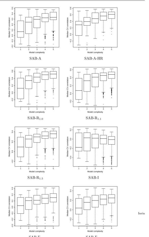
Templates. Denote V the pool of twelve variables specified by Eq. (9) to (19) (Table 1), plus the iRMSD defined in the SAB. Let a template be a set of variables, i.e. a subset of V. To define parsimonious templates from the set V, we generate subsets of V involving up to at most five variables–an upper bound dictated by the fact that beyond five variable, the performance of the corresponding best predictive model starts to decrease (supplemental Fig. 6). This defines a pool of templates T = {T1, . . . , T1585}2.
Cross-validation. In the following a model is associated to both a template Tl ∈ T and a dataset D from the SAB. More precisely, a model refers to a linear model, i.e. the variables of the template plus the associated coefficients.
Practically, models are defined during k-fold cross-validation (with k = 5), and a number of NXV (=10000) of repetitions (Fig. 2). Consider one repetition, which thus consists of splitting at random D into 5 subsets called folds. For one fold, a linear model associated with Tlis trained on 4/5 of the dataset D, and predictions are run on the remaining 1/5 of complexes. Processing the five folds yields one repetition of the cross validation procedure, resulting in one prediction ˆ
gij for the ∆Gexpd i of each complex. The set of all predictions in one repeat, say the jth one, is denoted
ˆ
Gj={ˆgij}i=1,...,|D|. (2) Note again that these predictions stem from k linear models associated with Tl, namely one per fold.
Statistics per template. Considering one cross-validation repetition, we define the correlation Corrj as the correlation between the experimental values {∆Gexpd i} and the predictions ˆGj. An overall assessment of the template Tl using the NXV repetitions is obtained by the following median of correlations(see also the supplemental Section 6.4.3):
C[Tl,D] = medianj Corrj. (3)
For a complex, we define the binding affinity prediction ˆgi as the median across repetitions i.e. ˆ
gi=medianj gˆij. (4)
Likewise, the median prediction error is defined by
ei≡ ei[Tl,D] = medianj(∆Gexpd i− ˆgij), (5) 2Since we have 12 variables, one has P5
k=1 12
and the median absolute prediction error by: eabs
i ≡ eabsi [Tl,D] = medianj(|∆Gexpd i− ˆgij|). (6) Using this latter value, we define the prediction ratio perror
δ as the percentage of cases such that the dissociation free energy is off by a specified amount δ:
perror
δ = %cases in D such that eabsi [Tl,D] ≤ δ. (7) In particular, setting δ to 1.4, 2.8 and 4.2 kcal/mol in the previous equation yields cases whose Kd is approximated within one, two and three orders of magnitude respectively.
Finally, a permutation test yields a p-value for each predictive model [41]. In a nutshell, the rationale consists of generating randomized datasets by shuffling their ∆Gexpi
d values. Then, one computes a performance criterion for each such dataset, from which the p-value is inferred (supplement, Algorithm 1).
Model selection. Define the best predictive model as the one maximizing the median corre-lation C[Tl,D] (Eq. (3)), called the performance criterion for short in the sequel.
We wish to single out the best predictive models, i.e. those that cannot be statistically distinguished from the best predictive model, as just defined.
To single out such models, observe that to compare two predictive models MTl and MTl0,
a univariate two-sample test suffices to check whether the two sets of performances (one per model) obtained for the NXV repetitions come from the same distribution (the null hypothesis H0), or whether one dominates the other. In an analogous spirit and since we are handling a pool of predictive models T , we wish to identify within T a subset of predictive models whose distribution cannot be distinguished from the best predictive model. To this end, we decompose the predictive models as T = T1∪ T2 such that (i) the best predictive model is in T1, (ii) in comparing two predictive models from T1, one does not reject H0, and (iii) in comparing one predictive model from T1 against one predictive model from T2, one rejects H0. The predictive models in T1 are called the specific models for the dataset D. The corresponding procedure is based on the Kruskal-Wallis test (supplemental, Algorithm 2). The p-value threshold is set to α = 0.01.
We also use the eight datasets to define the best overall predictive model. To this end, we sorted the models using the aforementioned performance criterion and took the model with lowest median rank among all datasets. This yields the predictive model 9 in the sequel.
3
Results
3.1
Specific predictive Models yield Enhanced Correlations. . .
Recall that a dataset can be the SAB or a subset of the SAB defined by bounds on the iRMSD or the resolution of complexes and partners. In the sequel, we analyze the performances of predictive models, as defined in the previous section.
Interestingly, a single predictive model is significantly better than the others for all datasets. These predictive models are all statistically significant with a p-value smaller than 0.01, except for the one associated with the dataset SAB-I, therefore omitted from subsequent analysis.
In terms of correlations between estimates and ∆Gexpi
d (supplemental Table 4, 5-fold cross validation), our specific predictive models outperform previous works in 5/8 cases. For two of the three remaining cases, the top correlation is provided by the complex model from [39],
which we estimated to use 94 variables (see supplemental Section 6.3.1). For the remaining one, [21] provides the best results with a seven variables model. Unfortunately, the corresponding variables are not specified.
In terms of correlation values themselves, three facts emerge. First, the predictive model specific of the high resolution model dataset yields a remarkable correlation of 0.77. Second, for flexible datasets, satisfactory performances are observed, which is unexpected since such cases are generally considered as the most challenging ones for affinity predictions. In particular, for flexible cases characterized by an interface iRMSD larger than 1.5Å, a correlation of 0.46 is obtained, a value comparable to that of the whole dataset, namely 0.48. Finally, the best overall predictive model, when challenged by individual datasets, shows performances comparable to those of their specific predictive models with maximum drop in correlation of 0.06. This is a clear assessment of its robustness.
3.2
. . . and Improved Predictions on a per Complex Basis
The correlation between predictions and ∆Gexpi
d provides a global performance assessment of a predictive model for a dataset. To gain insights at the individual complex level, we use the individual predictions ˆgij. Using these individual predictions, we compute the prediction ratio (Eq. 7) for δ = 1.4, 2.8 and 4.2 kcal/mol, respectively, yielding the fraction of cases for which Kd is predicted within one, two and three orders of magnitude. Three striking facts emerge from Table 3.
First, the merits of our specific predictive models as well as those of the best overall predictive model clearly emerge. As a quantitative measure, we collect the min and max prediction ratios for the aforementioned three values of δ, yielding a three pairs min-max percentages. For our best overall predictive model, one gets 44-57%, 74-86% and 91-95% within one, two and three orders of magnitude. In contrast, the intervals for [33] are 46-51%, 68-83% and 85-95%, and those for [30] are 22-44%, 57-73% and 85-93%. Collecting now the min and max prediction ratios of the specific predictive models on their specific datasets, one gets 46-62%, 78-89%, 85-97%. Thus, for the whole SAB, both the specific predictive model and the best overall predictive model yield improved performances.
Second, the prediction ratios of the predictive model specific of the high resolution dataset turn out to be 62%, 89% and 97% within one, two and three orders of magnitude, an outstanding performance.
Third, concerning the flexible datasets, considered as the most challenging ones in previous studies, predictive model 7 (dataset SAB-F1) and predictive model 8 (dataset SAB-F1.5) reach performances comparable to those obtained on the whole SAB, namely perror
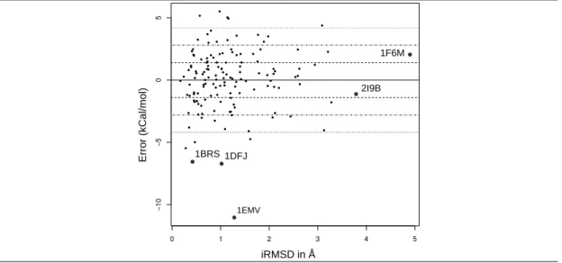
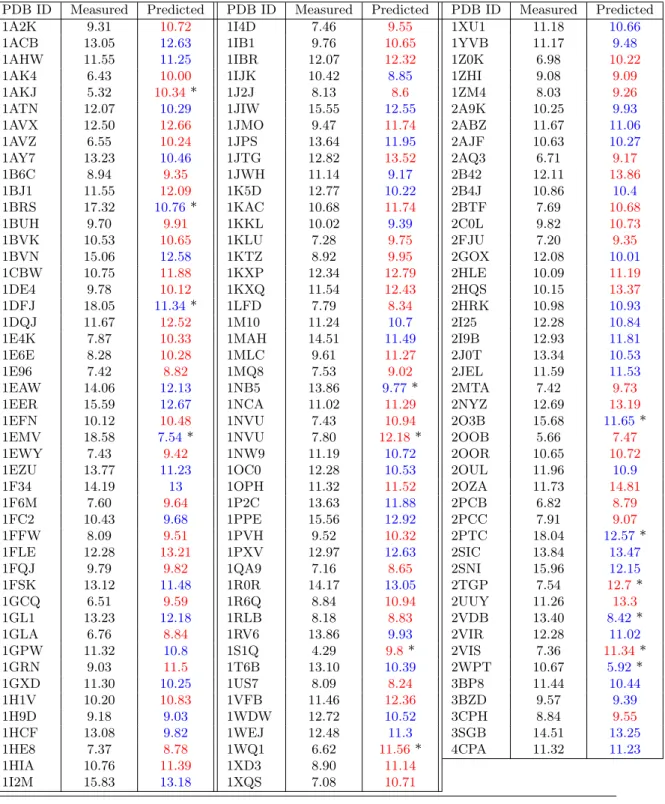
1.4 values of 50% and 50% respectively, instead of 47%. This shows that the difficulty of predicting binding affinity for flexible interfaces can be circumvented by the right choice of variables. This observation is also backed up by the lack of correlation between the interface flexibility and the prediction error (Fig. 3). We also note in passing that this conclusion is based on the analysis of the prediction ratios of Eq. (7), rather than that of the correlation coefficients of Eq. (3) (supplemental Table 4). Correlation coefficients are indeed global indicators of the dependency between two random variables, and do not assess the predictive performances on a per-complex basis. Specific cases. Inspecting extreme cases is informative (named cases, Fig. 3). The individual predictions ˆgi from Eq. 4 are provided in the supplemental Table 9.
On the one hand, the affinity of three complexes with subpicomolar affinity (1EMV, 1BRS, 1DFJ) is significantly under-estimated (Fig. 3). These three complexes involve an inhibitor taking the place of a cognate nucleic acid. Such complexes typically involve strong electrostatic
interactions [42, 30], which are overlooked by our models. It could also be the case that such complexes manage to limit the entropic loss upon binding, possibly by transferring the dynamics of interfacial atoms to the protein’s non interacting atoms.
On the other hand, predictions are excellent for several flexible cases, in particular 1F6M and 2I9B (Fig. 3). Complex 1F6M consists of a thioredoxin reductase in flavin-reducing conformation with its substrate. The reductase switches between bound and unbound conformations using a hinge-like motion. Complex 2I9B consists of a urokinase plasminogen activator receptor and its associated ligand. There is a global conformational change of the receptor upon binding (RMSD 2.657 Å) but no obvious hinge motion. It is the only complex with an iRMSD greater than 3 Å and a prediction error below 1.4 kcal/mol.
Classically for complexes with large interfaces, affinity predictions based on the BSA often result in overestimates. Beyond a certain interface size, the affinity no longer increases as much with the interface size, a behavior which could be related to a non-uniform atomic packing at the interface [30]. However, the packing distribution of large interfaces matches that of the remaining ones (supplemental Fig. 7), and no correlation is observed between the quality of individual predictions and interface size (supplemental Fig. 8). Thus, packing heterogeneity may not account for mild to poor prediction performances in that context.
Validation on external datasets. Cross validation results obtained on datasets of small size should be interpreted with care [25], and checks on external datasets are a must [38]. We therefore ran predictions on an external dataset (supplemental Table 7), from which two striking facts emerge.
The correlations observed compare to those obtained with cross-validation, with a maximum drop of 0.11 excluding predictive models 2 and 8. For the latter two predictive models, the drop reaches 0.33 and 0.25 respectively, a fact likely related to the small size of their training datasets. Second, the proportions perror
1.4 , perror2.8 and perror4.2 are smaller than their cross-validated counterparts, by a factor 1.4 (perror
4.2 , predictive model 8) to 9.5 (perror1.4 , predictive model 7). Therefore, on this external dataset, despite being good predictors on a global level, as assessed by the correlation coefficient, our predictive models do not always perform robustly on a per complex basis.
3.3
Accounting for Interface Morphology and Packing Boosts
Perfor-mances
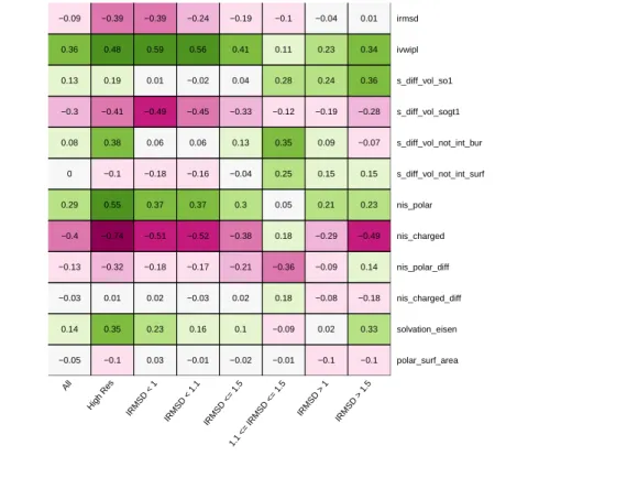
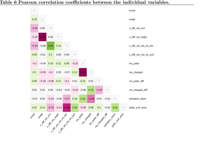
The performances of our predictive models owe to the new variables introduced in this study (Table 2). The variable selected most often is IVW-IPL (6/8 cases), stressing the role of the interface size (in terms of buried surface area), but also of atomic packing properties. The second variable selected most often is NIScharged (5/8 cases), highlighting the role of solvent interactions [30]. Two other variables selected for 3/8 datasets, respectively represent volume variation at the interface rim (SVD_SO1), and solvation properties of the complex at the atomic scale (ATOM_SOLV). Interestingly, inspecting these four variables reveals a correlation between IVW-IPL and SVD_SOGT1 (supplemental Table 6), so that these variables might be used interchangeably. The same observation holds for NIScharged and NISpolar.
Of particular interest in this context is our best overall predictive model. This predictive model uses variables IVW-IPL, SVD_SO1 and NISchargedand is therefore equivalent to predic-tive model 4. Not surprisingly, these variables form the top three of variables selected most often by the specific predictive models (Table 2). Its performances, are similar to those of specific
predictive models on their own datasets (Table 3). Interestingly, it is a better predictor of flex-ible complexes than predictive model 1. Finally, its results on external datasets (Tables 7 and 8) show that it is outperformed by specific predictive models for four datasets, and outperforms them for two (not considering predictive model 6).
4
Discussion and Outlook
This work develops sparse binding affinity predictions models, which shed new light on the hardness of affinity prediction, and improve prediction quality using variables coding enthalpic and entropic variations upon binding.
On the hardness of affinity predictions. Flexible datasets have been reported as the most challenging ones in previous studies. However, as shown here, the segregation of flexible versus rigid appears partially founded, with some easy to predict flexible complexes, and some hard to predict rigid cases. This observation is not completely surprising, since conformational changes alone tell little, in particular, on entropic changes upon binding. It also hints at the possibility of improving the quality of predictions for cases with small conformational changes upon binding, as molecular dynamics simulations in the intermediate time range may provide good estimates for the entropic penalties in those cases.
On the quality of predictions. A key achievement of this study is the quality of predictions, assessed in terms of absolute error or equivalently accuracy on Kd. To summarize, two values may be put forward, namely the fraction of cases for which Kd is predicted within one and two orders of magnitude. For the best overall predictive model, these fractions, corresponding to the whole SAB, are 48% and 79%, respectively. For the predictive model specific of high resolution complexes, these fractions are 62% and 89%. These numbers clearly advance the state-of-the-art, and call for two comments.
First, our models do not take into account the pH, whose change by two units may alter Kd by a factor ten or more. Given this specificity, they second the goal set in [30], namely that of approximating Kd within two orders of magnitude.
Second, the high performance obtained for high resolution structures recalls the short range nature of selected forces–van der Waals interactions in particular, and stresses the dependence of energies on atomic details. From a quantitative standpoint, from Cruickshank’s formula, the typical precision on atomic coordinates at a resolution of say 2.5Å lies in the range [0.2, 0.4] Å [17, 2]. At such a resolution, which is the worst used in the high resolution dataset (supplemental Fig. 5), the inter-atomic distance between non covalently bonded atoms located nearby in 3D space [10] may already be spoiled by a factor circa ∼ 1/4 (say 2 × 0.3/2.5). The situation dete-riorates with the resolution, with a potential significant impact on the atomic scale parameters listed in Table 1. Therefore, the incidence of resolution on prediction performance should not come as a surprise. In a more general perspective, this observation is reminiscent of the role of molecular shape in determining motions [36], and also on the importance of packing properties in protein structure [11].
One generic predictive model versus several specific predictive models. The diversity of the specific predictive models may be seen as a weakness or a strength. For the former viewpoint, one may argue that thermodynamics call for a unified model. For the latter one, given the intrinsic complexity of the problem (recall that the binding affinity is inherently coupled to a thermodynamic equilibrium), and the paucity of the dataset, it is clearly beneficial to exploit
specific features of datasets. Moreover, specific predictive models are of practical interest since to predict the affinity of a complex performing a specific biological function, one may use a dataset of complexes related to that function. Further arguments to choose between these two interpretations will likely emerge upon populating the structure affinity benchmark.
On key parameters. Our predictive models preferably use parameter IVW-IPL, and then NIScharged. The former, introduced in this work, combines the overall shape of the interface and involves atomic packing properties. It is reminiscent of cooperativity phenomena observed for weak interactions [5]. The latter, NIScharged, encodes the electrostatic properties of the non interacting surface, as recently investigated [49]. The following top scorers represent volume variation at the interface rim (SVD_SO1), and solvation properties of the complex at the atomic scale (ATOM_SOLV). Among these four variables, two describe surface properties at different scales (atomic for ATOM_SOLV, and at residue level for NIScharged), and two encode interface properties, one static for the whole interface (IVW-IPL), and one dynamic for the outer layer of the interface (SVD_SO1).
Remarkably, these parameters are simple ones, derived from the Voronoi diagram of the solvent accessible models of the three structures involved (two for the partners, one for the complex). From a computational standpoint, processing a structure of say up to 10,000 atoms takes a handfull of seconds on a desktop computer [9].
Outlook. Estimating binding affinities is a central endeavor to understand protein - protein interactions. Strikingly, the predictive models and variables presented here yield a prediction accuracy of 2.8 kcal/mol per complex in 79% of cases for the whole SAB, and in 89% of cases for high resolution complexes. This represent a significant progress over previous methods. Since our methods inherently exploit static properties of crystal structures, improving results even further calls for developments in two directions. On the one hand, unveiling dynamical properties of the partners and the associated complex, by sampling and modeling the associated (potential, free) energy landscapes will undoubtedly yield enhanced predictions [50]. Along the way, a central problem to be addressed is that of the potential energy model best suited, since, as shown in this work, coarse grain descriptors can match or surpass the performances of detailed chemical ones. In this respect, our ability to accurately sample [50, 13] and compare [8] sampled energy landscapes should prove critical. On the other hand, a weakness shared by our method and previous ones is the absence of terms taking into account the pH and the ionic strength – a limitation actually accounting for the poor performances observed on complexes involving significant electrostatic interactions. For such cases, incorporating terms accounting for counter-ion condensation seems critical, yet, controlling the enthalpy - entropy balance within such models remain challenging [42, 46].
The affinity prediction problem is also of special interest from the machine learning perspec-tive. Affinity prediction is indeed modeled here a particular instance of a problem known as regression [28]. In this setting, the data is assumed to be generated by a process and applied some random noise. The most important attribute of regressors is their consistency, i.e. their ability to converge toward the true model given data accounting for the whole space. However, for a regressor to achieve consistency, the data must satisfy some assumptions. For instance it should be well distributed over the space of possible data points. In our case, this means that the dataset should evenly represent all possible protein-protein complexes. This is most probably not the case for the SAB. The availability of larger datasets will also ease the model selection problem, undertaken by complete enumeration over the parameter set in this work. In principle, sparse least square models can be obtained using regularization techniques [48]. However, the in-herent randomization used by cross-validation makes model selection unstable for small datasets,
making such methods hard to use at this stage. For these reasons, sparse specific models using with relevant variables, as developed in this work, appear as a privileged solution to estimate binding affinities.
5
Artwork
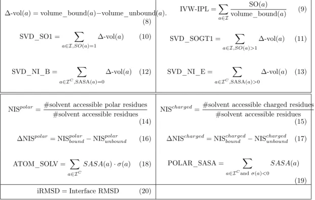
Table 1 Parameters used to estimate binding affinities. Atomic level param-eters: IVW-IPL, SVD_SO1, SVD_SOGT1, SVD_NI_B, SVD_NI_E, ATOM_SOLV, POLAR_SASA; Residue level parameters: NISpolar, NIScharged, ∆NISpolar, ∆NIScharged; In-terface level parameter: iRMSD. The acronyms read as follows (see text for details): Sum of Volume Differences; Shelling Order; Inverse Volume Weighted; Internal Path Length; Non Interacting Buried/Exposed; Non Interacting Surface; Solvent Accessible Surface Area;
∆-vol(a) = volume_bound(a)−volume_unbound(a). (8) IVW-IPL =X a∈I SO(a) volume_bound(a) (9) SVD_SO1 = X a∈I,SO(a)=1 ∆-vol(a) (10) SVD_SOGT1 = X a∈I,SO(a)>1 ∆-vol(a) (11) SVD_NI_B = X a∈IC ,SASA(a)=0 ∆-vol(a) (12) SVD_NI_E = X a∈IC ,SASA(a)>0 ∆-vol(a) (13)
NISpolar=#solvent accessible polar residues
#solvent accessible residues (14)
NIScharged= #solvent accessible charged residues
#solvent accessible residues (15)
∆NISpolar=NISpolar
bound− NIS
polar
unbound (16) ∆NIScharged=NIS
charged bound − NIS charged unbound (17) ATOM_SOLV = X a∈IC
SASA(a)· σ(a) (18) POLAR_SASA = X
a∈ICandσ(a)<0
SASA(a) (19)
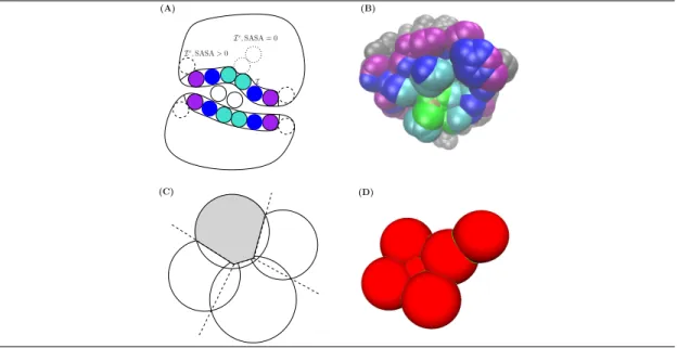
Figure 1 Structural parameters used in this work. (A)Labeling the atoms, illustration on a fictitious 2D complex. The binding patch on each partner consists of one layer of atoms (I, colored solid balls), as identified by a Voronoi interface model [10, 35]. The non interface atoms (Ic) are split into those which retain solvent accessibility (SASA > 0, dashed balls), and those which do not (SASA = 0, dotted balls) (B) Each interface atom is assigned an integer, its shelling order, equal to the smallest number of atoms traveled to reach an exposed non interface atom, i.e. an atom belonging to Ic and with SASA > 0 (in grey) [5]. (C,D) The volume of an atom is defined as the volume of the intersection between its ball in the solvent accessible model, and its Voronoi cell [9], a quantity well defined even if the atom retains solvent accessibility. The packing of this atom is the inverse of this volume. Practically, interfaces and binding patches are computed with Vorshell[35], while atomic surface areas and volumes are computed with Vorlume[9]. Both programs are available from the Structural Bioinformatics Library (SBL), see http://sbl.inria.fr. Ic, SASA = 0 Ic, SASA > 0 I (A) (B) (C) (D)
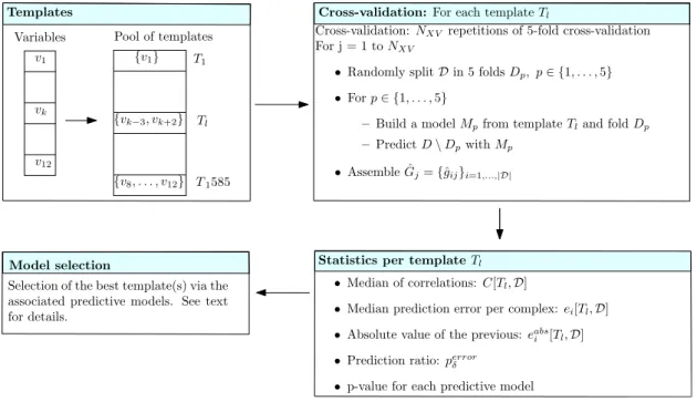
Figure 2 Running binding affinity predictions for a dataset D i.e. a subset of the structure affinity benchmark: graphical outline of the statistical methodology. (Tem-plates)From the pool of variables, templates are generated. (Cross-validation) Each template undergoes a number NXV of repetitions of 5-fold cross-validation, yielding one binding affinity prediction per complex for each repetition. (Statistics) Various statistics are computed to as-sess the performances yielded by the predictive model associated to each template. (Model selection)Predictive models are compared, and the best ones selected.
T1 T1585 Pool of templates v1 vk v12 {v1} {v8, . . . , v12} Variables {vk−3, vk+2} Tl
Cross-validation: NXV repetitions of 5-fold cross-validation
For j = 1 to NXV
• Randomly split D in 5 folds Dp, p∈ {1, . . . , 5}
• For p ∈ {1, . . . , 5}
– Build a model Mpfrom template Tland fold Dp
– Predict D\ Dpwith Mp
• Assemble ˆGj={ˆgij}i=1,...,|D|
Cross-validation: For each template Tl
Model selection
• Median of correlations: C[Tl,D]
• Median prediction error per complex: ei[Tl,D]
• Absolute value of the previous: eabs i [Tl,D]
• Prediction ratio: perror δ
• p-value for each predictive model Selection of the best template(s) via the
associated predictive models. See text for details.
Statistics per template Tl
Templates
Table 2 Parameters used by the best predictive model for a given dataset. A dataset is a subset of the structure affinity benchmark. A specific predictive model is the predictive model which performed significantly better than all the others for a given dataset during model selection. The parameters are those from Table 1. Black dots mark variables used by statistically significant predictive models and white dots those used by other predictive models. The last column counts the number of statistically significant predictive models using a given parameter. Asterisks identify atomic level parameters.
Predictive Predictive Predictive Predictive Predictive Predictive Predictive Predictive
Model 1 Model 2 Model 3 Models 4 and 9 Model 5 Model 6 Model 7 Model 8 Counts
SAB-A SAB-A-HR SAB-R1.0 SAB-R1.1 SAB-R1.5 SAB-I SAB-F1 SAB-F1.5
iRMSD • 1 IVW-IPL∗ • • • • • • 6 SVD_SO1∗ • • • 3 SVD_SOGT1∗ • 1 SVD_NI_E∗ • 1 SVD_NI_B∗ • ◦ 1 (2) NISpolar • 1 NIScharged • • • • • 5 ∆NISpolar ◦ (1) ∆NIScharged ATOM_SOLV∗ • • • 3 POLAR_SASA∗
T able 3 Datasets and th e ir sp e cific predictiv e mo dels: p erformances in estimating the d isso ciation free energy ∆ Gd . Eac h predictiv e mo del (ro ws) w as tested on eac h dataset (columns). A cell in the Table features the values of the affinit y prediction ratio p error 1.4 , p error 2.8 and p error 4.2 resp ectiv ely ,see Eq. (7). For ins tance, Predic ti ve Mo del 1, whe n ev aluated on data set SAB-A (139 complexes) predicted 47.48%, 78.42% and 92.09% of the complexes with a median absolute error belo w 1.4, 2.8 and 4.2 kcal/mol, resp ectiv ely . Equiv alen tly , these are the fractions of cases suc h that Kd is estimated within one, tw o and three orders of magnitude. (T op part) Previous w ork. Lines mark ed with Rep. (replica) w ere obtained using using the values of the parameters pro vided in the SAB for [30] and those pro vided by the authors (p ersonal comm unication) for [33], along with their res pectiv e proto cols. Lines not mark ed with Rep. w ere obtained usin g th e variables of the original mo dels, within our setup. (Bottom part) Our predictiv e mo dels. Bold values indicate when a predictiv e mo del w as tested on its sp ecific dataset. SAB-A SAB-A-HR SAB-R 1 .0 SAB-R 1 .1 SAB-R 1 .5 SAB-I SAB-F 1 SAB-F 1 .5 (1) [30, Janin ,rep] 29.63, 60.74, 77.78 -37.33, 76.00, 92.00 -37.04, 62.96, 85.19 -6.06, 24.24, 39.39 (2) [30, Janin ] 39.57, 64.75, 89.21 44.12, 72.06, 92.65 37.18, 73.08, 91.03 39.05, 71.43, 90.48 39.57, 64.75, 89.21 37.14, 71.43, 88.57 32.35, 67.65, 85.29 21.62, 56.76, 86.49 (3) [33, K as tr itis, rep] 46.85, 76.92, 90.21 -41.67, 80.56, 90.28 -48.62, 81.65, 91.74 -41.18, 61.76, 85.29 (4) [33, K as tr itis] 46.76, 75.54, 88.49 51.35, 75.68, 94.59 45.59, 80.88, 91.18 48.72, 80.77, 93.59 47.62, 82.86, 91.43 46.76, 75.54, 88.49 50.00, 72.86, 85.71 47.06, 67.65, 85.29 (5) Predictiv e Mo del 1 47.48, 78.42, 92.09 56.76, 86.49, 94.59 54.41, 77.94, 92.65 53.85, 80.77, 91.03 47.62, 79.05, 91.43 44.44, 62.96, 85.19 44.29, 77.14, 92.86 47.06, 70.59, 97.06 (6) Predictiv e Mo del 2 47.48, 77.70, 90.65 62.16, 89.19, 97.30 41.18, 76.47, 89.71 44.87, 79.49, 88.46 40.95, 76.19, 90.48 29.63, 70.37, 85.19 47.14, 77.14, 88.57 55.88, 73.53, 91.18 (7) Predictiv e Mo del 3 48.92, 78.42, 91.37 54.05, 83.78, 94.59 51.47, 82.35, 92.65 55.13, 79.49, 91.03 45.71, 80.95, 91.43 37.04, 70.37, 88.89 48.57, 74.29, 91.43 52.94, 79.41, 91.18 (8) Predictiv e Mo dels 4 and 9 48.20, 79.14, 91.37 51.35, 86.49, 94.59 57.35, 79.41, 91.18 55.13, 79.49, 91.03 43.81, 77.14, 91.43 40.74, 66.67, 88.89 48.57, 74.29, 92.86 52.94, 79.41, 91.18 (9) Predictiv e Mo del 5 42.45, 76.98, 89.93 56.76, 81.08, 89.19 57.35, 79.41, 89.71 55.13, 80.77, 88.46 45.71, 80.00, 89.52 40.74, 74.07, 88.89 47.14, 75.71, 88.57 41.18, 70.59, 85.29 (10) Predictiv e Mo del 6 37.41, 64.03, 87.05 37.84, 64.86, 83.78 36.76, 55.88, 88.24 34.62, 56.41, 87.18 37.14, 66.67, 85.71 44.44, 70.37, 88.89 35.71, 68.57, 87.14 32.35, 67.65, 88.24 (11) Predictiv e Mo del 7 48.92, 79.14, 91.37 59.46, 83.78, 91.89 54.41, 77.94, 91.18 52.56, 78.21, 91.03 46.67, 79.05, 91.43 37.04, 66.67, 85.19 50.00, 78.57, 90.00 50.00, 73.53, 94.12 (12) Predictiv e Mo del 8 38.85, 74.82, 89.93 32.43, 70.27, 89.19 48.53, 79.41, 88.24 44.87, 78.21, 87.18 39.05, 74.29, 89.52 33.33, 74.07, 88.89 47.14, 72.86, 90.00 50.00, 79.41, 85.29
Figure 3 The hardness of predicting a binding affinity does not correlate with the flexibility of the complex. x-axis: flexibility of the interface, expressed in terms of interface iRMSD; y-axis: median prediction error ei[Tl,D] (Eq. (5)). Dashed, dash-dotted and dotted lines respectively show errors of ±1.4, ±2.8, ±4.2 kcal/mol, corresponding to Kd approximated within one, two and three orders of magnitude.
● ● ● ● ● ● ● ● ● ● ● ● ● ● ● ● ● ● ● ● ● ● ● ● ● ● ● ● ● ● ● ● ● ● ● ● ● ● ● ● ● ● ● ● ● ● ● ● ● ● ● ● ● ● ● ● ● ● ● ● ● ● ● ● ● ● ● ● ● ● ● ● ● ● ● ● ● ● ● ● ● ● ● ● ● ● ● ● ● ● ● ● ● ● ● ● ● ● ● ● ● ● ● ● ● ● ● ● ● ● ● ● ● ● ● ● ● ● ● ● ● ● ● ● ● ● ● ● ● ● ● ● ● ● ● ● ● ● ● 0 1 2 3 4 5 −10 −5 0 5 1BRS 1DFJ 1EMV 2I9B 1F6M iRMSD in Å Err or (kCa l/mol)
References
[1] R. Bahadur, P. Chakrabarti, F. Rodier, and J. Janin. A dissection of specific and non-specific protein–protein interfaces. JMB, 336(4):943–955, 2004.
[2] D. Blow. Outline of crystallography for biologists. Oxford University Press, 2002.
[3] J.-D. Boissonnat and M. Yvinec. Algorithmic geometry. Cambridge University Press, UK, 1998. Translated by H. Brönnimann.
[4] L. Bonetta. Protein-protein interactions: Interactome under construction. Nature, 468(7325):851–854, 2010.
[5] B. Bouvier, R. Grunberg, M. Nilgès, and F. Cazals. Shelling the Voronoi interface of protein-protein complexes reveals patterns of residue conservation, dynamics and composi-tion. Proteins: structure, function, and bioinformatics, 76(3):677–692, 2009.
[6] B.R. Brooks, R.E. Bruccoleri, B.D. Olafson, D.J. States, S. Swaminathan, and M. Karplus. CHARMM: A program for macromolecular energy, minimization, and dynamics calcula-tions. journal of computational chemistry. Volume 4, Issue 2, Pages 187 - 217, 1983. [7] F. Cazals and T. Dreyfus. SBL, the Structural Bioinformatics Library, 2015.
http://sbl.inria.fr.
[8] F. Cazals, T. Dreyfus, D. Mazauric, A. Roth, and C.H. Robert. Conformational ensem-bles and sampled energy landscapes: Analysis and comparison. Journal of Computational Chemistry, 36(16):1213–1231, 2015.
[9] F. Cazals, H. Kanhere, and S. Loriot. Computing the volume of union of balls: a certified algorithm. ACM Transactions on Mathematical Software, 38(1):1–20, 2011.
[10] F. Cazals, F. Proust, R. Bahadur, and J. Janin. Revisiting the Voronoi description of protein-protein interfaces. Protein Science, 15(9):2082–2092, 2006.
[11] T.C. Chalikian. Volumetric properties of proteins. Annual review of biophysics and biomolec-ular structure, 32(1):207–235, 2003.
[12] C.A. Chia-en, W. Chen, and M.K. Gilson. Ligand configurational entropy and protein binding. PNAS, 104(5):1534–1539, 2007.
[13] C. Chipot. Frontiers in free-energy calculations of biological systems. Wiley Interdisciplinary Reviews: Computational Molecular Science, 4(1):71–89, 2014.
[14] John D Chodera and David L Mobley. Entropy-enthalpy compensation: role and ramifica-tions in biomolecular ligand recognition and design. Biophysics, 42, 2013.
[15] C. Chothia and J. Janin. Principles of protein-protein recognition. Nature, 256:705–708, 1975.
[16] W. Cornell, P. Cieplak, C. Bayly, I. Gould, K. Merz, D. Ferguson, D. Spellmeyer, T. Fox, J. Caldwell, and P. Kollman. A second generation force field for the simulation of pro-teins, nucleic acids, and organic molecules. Journal of the American Chemical Society, 117(19):5179–5197, 1995.
[17] DWJ. Cruickshank. Remarks about protein structure precision. Acta Crystallographica Section D: Biological Crystallography, 55(3):583–601, 1999.
[18] J. Dunitz. Win some, lose some: enthalpy-entropy compensation in weak intermolecular interactions. Chemistry & biology, 2(11):709–712, 1995.
[19] D. Eisenberg and A.D. McLachlan. Solvation energy in protein folding and binding. Nature, 319:199–203, 1986.
[20] David Eisenberg, Morgan Wesson, and Mason Yamashita. Interpretation of protein folding and binding with atomic solvation parameters. Chem. Scr. A, 29:217–221, 1989.
[21] A. Erijman, E. Rosenthal, and J.M. Shifman. How structure defines affinity in protein-protein interaction. PLOS one, 9(10), 2014.
[22] D. Frenkel and B. Smit. Understanding molecular simulation. Academic Press, 2002. [23] M. Gerstein and F.M. Richards. Protein geometry: volumes, areas, and distances. In M. G.
Rossmann and E. Arnold, editors, The international tables for crystallography (Vol F, Chap. 22), pages 531–539. Springer, 2001.
[24] M.K. Gilson and H-X. Zhou. Calculation of protein-ligand binding affinities. Annual review of biophysics and biomolecular structure, 36(1):21, 2007.
[25] A. Golbraikh and A. Tropsha. Beware of q2! Journal of Molecular Graphics and Modelling, 20(4):269–276, 2002.
[26] M. Guharoy and P. Chakrabarti. Conservation and relative importance of residues across protein-protein interfaces. PNAS, 102(43):15447–15452, Oct 2005.
[27] W.F. Van Gunsteren and H.J.C. Berendsen. Groningen molecular simulation (GROMOS). Library manual, Biomos, Groningen, The Netherlands, pages 1–221, 1987.
[28] L. Györfi and A. Krzyzak. A distribution-free theory of nonparametric regression. Springer, 2002.
[29] N. Horton and M. Lewis. Calculation of the free energy of association for protein complexes. Protein Science, 1(1):169–181, 1992.
[30] J. Janin. A minimal model of protein–protein binding affinities. Protein Science, 23(12):1813–1817, 2014.
[31] J. Janin, R. P. Bahadur, and P. Chakrabarti. Protein-protein interaction and quaternary structure. Quarterly reviews of biophysics, 41(2):133–180, 2008.
[32] P.L. Kastritis, I.H. Moal, H. Hwang, Z. Weng, P.A. Bates, A. Bonvin, and J. Janin. A structure-based benchmark for protein-protein binding affinity. Protein Science, 20:482– 491, 2011.
[33] P.L. Kastritis, J.P.G.L.M. Rodrigues, G.E. Folkers, R. Boelens, and A.M.J.J. Bonvin. Pro-teins feel more than they see: Fine-tuning of binding affinity by properties of the non-interacting surface. J.M.B., 426:2632–2652, 2014.
[34] S.M. Lippow, K.D. Wittrup, and B. Tidor. Computational design of antibody-affinity im-provement beyond in vivo maturation. Nature biotechnology, 25(10):1171–1176, 2007.
[35] S. Loriot and F. Cazals. Modeling macro-molecular interfaces with Intervor. Bioinformatics, 26(7):964–965, 2010.
[36] M. Lu and J. Ma. The role of shape in determining molecular motions. Biophysical journal, 89(4):2395–2401, 2005.
[37] G. Meng, N. Arkus, M.P. Brenner, and V.N. Manoharan. The free-energy landscape of clusters of attractive hard spheres. Science, 327(5965):560–563, 2010.
[38] I. Moal and J. Fernández-Recio. Comment on protein-protein binding affinity prediction from amino acid sequence. Bioinformatics (Oxford, England), 2014.
[39] I.H. Moal, R. Agius, and P.A. Bates. Protein–protein binding affinity prediction on a diverse set of structures. Bioinformatics, 27(21):3002–3009, 2011.
[40] I. Moreira, P. Fernandes, and M.J. Ramos. Hot spots – a review of the protein–protein inter-face determinant amino-acid residues. Proteins: Structure, Function, and Bioinformatics, 68(4):803–812, 2007.
[41] B. Phipson and G.K. Smyth. Permutation p-values should never be zero: calculating exact p-values when permutations are randomly drawn. Statistical Applications in Genetics and Molecular Biology, 9(1), 2010.
[42] P. Privalov, A. Dragan, and C. Crane-Robinson. Interpreting protein/dna interactions: distinguishing specific from non-specific and electrostatic from non-electrostatic components. Nucleic acids research, page gkq984, 2010.
[43] D. Rajamani, S. Thiel, S. Vajda, and C.J. Camacho. Anchor residues in protein-protein interactions. PNAS, 101(31):11287–11292, 2004.
[44] G. Subba Rao, R. Vijayakrishnan, and M. Kumar. Structure-based design of a novel class of potent inhibitors of inha, the enoyl acyl carrier protein reductase from mycobacterium tuberculosis: A computer modelling approach. Chemical biology & drug design, 72(5):444– 449, 2008.
[45] F. Rodier, R.P. Bahadur, P. Chakrabarti, and J. Janin. Hydration of protein - protein interfaces. Proteins, 60(1):36–45, 2005.
[46] H. Schiessel. Counterion condensation on flexible polyelectrolytes: dependence on ionic strength and chain concentration. Macromolecules, 32(17):5673–5680, 1999.
[47] A. Schmidt, H. Xu, A. Khan, T. O’Donnell, S. Khurana, L. King, J. Manischewitz, H. Gold-ing, P. Suphaphiphat, A. Carfi, E. Settembre, P. Dormitzer, T. Kepler, R. Zhang, A. Moody, B. Haynes, H-X. Liao, D. Shaw, and S. Harrison. Preconfiguration of the antigen-binding site during affinity maturation of a broadly neutralizing influenza virus antibody. PNAS, 110(1):264–269, 2013.
[48] R. Tibshirani. Regression shrinkage and selection via the lasso. Journal of the Royal Sta-tistical Society. Series B (Methodological), pages 267–288, 1996.
[49] K.M. Visscher, P.L. Kastritis, and A. Bonvin. Non-interacting surface solvation and dynam-ics in protein–protein interactions. Proteins, 83:445–458., 2015.
[51] Z. Yand, L. Guo, L. Hu, and J. Wang. Specificity and affinity quantification of protein -protein interactions. Bioinformatics, 29(9):1127–1133, 2013.
6
Supplemental
6.1
Datasets from the Structure Affinity Benchmark
Curation. To exploit variation of structural parameters between the unbound and bound form, we establish a one-to-one correspondence between the atoms of a partner (from bound to un-bound). To cope with cases involving missing residues or atoms, we proceed in two stages. First, we perform an alignment and map residues of the bound and unbound chains. Second, we map atoms of paired residues. We then retain the cases for which at least 80% of atoms are paired. This procedure ruled out two cases, namely 1E6J (78%) and 1ZLI (76%). We also removed three cases (1IQD, 1NSN, 1UUG) for which an upper bound on Kd instead of a proper value is provided for a total of 139 complexes.
Datasets. The various datasets defined in previous works from the SAB are presented on Fig. 4.
Figure 4 The various datasets defined from the structure affinity benchmark (SAB), based on iRMSD between the unbound and bound structures.
0 1˚A 1.1˚A 1.5˚A iRMSD SAB-F1.1 SAB-F1.5 SAB-R1.5 SAB-R1.1 SAB-R1 SAB-I
The datasets depicted on Fig. 4 are defined as follows: • SAB-A (139 complexes): all complexes.
• SAB-R1.0 (68 complexes): (focus on ridigity, strict threshold) complexes characterized by iRMSD < 1Å [39] ([33] and [51] used iRMSD ≤ 1Å, 69 complexes).
• SAB-R1.1(78 complexes): (focus on ridigity, intermediate threshold) complexes character-ized by iRMSD < 1.1Å [30].
• SAB-R1.5 (105 complexes): (focus on ridigity, relaxed threshold) complexes characterized by iRMSD ≤ 1.5Å [33].
• SAB-I (27 complexes): (intermediate complexes) complexes characterized by 1.1 ≤ iRMSD ≤ 1.5Å [30].
• SAB-F1 (70 complexes): (focus on flexibility, relaxed threshold) complexes characterized by iRMSD > 1Å [51] ([39] used iRMSD ≥ 1Å, 71 complexes)
• SAB-F1.5 (34 complexes): (focus on flexibility, strict threshold) complexes with iRMSD > 1.5Å [30][33].
To which we add:
6.2
Resolution of Crystal Structures in the Affinity Benchmark
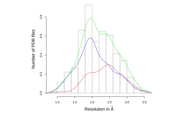
The distribution of resolutions of crystal structures found in the SAB is presented on Fig. 5. Figure 5 Resolution of the structures in the SAB.The histogram and green kernel density estimation curve are for the whole SAB, the red curve is for the complexes and the blue curve is for the unbound partners. For the whole SAB: Minimum = 0.93 Å, median: = 2.13 Å, average = 2.19 Å, max = 3.5 Å. NB: the high resolution dataset SAB-A-HR retains only entries whose resolution is better than 2.5 Å for both the complex and the individual partners [21].
Resolution in A° Number of PDB files 1.0 1.5 2.0 2.5 3.0 3.5 0.0 0.2 0.4 0.6 0.8
6.3
Methods used in Previous Studies
This section reviews previous work on affinity prediction, in three respects: the type of prediction model used, the variables used, and the statistical methodology.
6.3.1 From reference [39]
Datasets. Seven complexes were discarded from the original affinity benchmark: three because only the upper bound of the affinity was known (1UUG, 1IQD and 1NSN) and four because some features needed by the models were missing (1DE4, 1M10, 1NCA and 1NB5).
Types of models. Affinity values were predicted as the un-weighted average of the output of four different classifiers (random forest, multivariate adaptive regression splines, M5’ regression trees and radial basis function interpolation). Each classifier was fed a total of 200 different and possibly correlated features. All classifiers were able to perform feature selection to some extent
and therefore, their actual number of parameter was smaller than 200. In effect, M5’ trees use 84 variables, random forest uses 19 variables, MARS uses 10 variables and RBF weights all variable equally and therefore virtually uses all 200 variables. The union of the three first sets contains 94 variables.
Type of variables. The variables used fall into 7 categories: • Statistical potentials (both atomistic and coarse-grained) • Solvation and electrostatics (using force fields)
• Entropy terms (translational, rotational, vibrational)
• Contact potentials (H-bonds, π-π) interactions, Van der Waals, salt bridges) • Interface properties (BSA, polarity, geometrical features, surface complementarity) • Change between bound and unbound states for all of the above
• All of the above computed on an ensemble of structures generated with CONCOORD. Type of cross validation. On the training set, the correlation between predictions and ex-perimental values was computed using a cross-validation. Complexes from the test set were predicted using the model trained on the validated set. The models were trained on a subset of 57 complexes with further validated affinity values. The predictions were tested on the training dataset using leave-one-out cross-validation. They were further tested on 80 complexes. How-ever, the reported results do not include the correlation between predictions and affinity on the test set alone. Instead, the correlations were reported for the test set + cross-validated train set. 6.3.2 From reference [30]
Datasets. The set of rigid complexes (with iRMSD < 1.1 ) minus six complexes (1UUG, 2PTC, 1BRS, 2BTF, 1Z0K and 1S1Q) was used to fit the model. In SAB-I, four more complexes were also removed: 1EMV, 1KXP, 1AKJ and 1WQ1.
Type of model. A linear model was fitted on the data using least-square regression.
Type of variables. Two variables were used for that model: iRMSD and the buried surface area. Both are interface properties.
Type of cross-validation. No cross-validation was involved. The correlation between fitted and experimental values was computed on various subset of the SAB and the whole SAB. The results are therefore optimistic on rigid complexes.
Remarks In various datasets, complexes which were badly predicted by the model were re-moved as outliers. This leads to artificially high correlation coefficients. This is denoted by yellow cells in Table 4.
6.3.3 From reference [51]
This paper first aims at creating a scoring function for docking using statistical parameters. The correlation between the score of a complex and its affinity was also computed.