UNIVERSITÉ DE MONTRÉAL
METHODOLOGY AND TOOLS TO MAKE PREDICTIONS FROM SPORADIC DELIVERY DATA
PAUL MURRAY
DÉPARTEMENT DE MATHÉMATIQUES ET DE GÉNIE INDUSTRIEL ÉCOLE POLYTECHNIQUE DE MONTRÉAL
THÈSE PRÉSENTÉE EN VUE DE L’OBTENTION DU DIPLÔME DE PHILOSOPHIAE DOCTOR
(GÉNIE INDUSTRIEL) MAI 2018
UNIVERSITÉ DE MONTRÉAL
ÉCOLE POLYTECHNIQUE DE MONTRÉAL
Cette thèse intitulée :
METHODOLOGY AND TOOLS TO MAKE PREDICTIONS FROM SPORADIC DELIVERY DATA
présentée par : MURRAY Paul
en vue de l’obtention du diplôme de : Philosophiae Doctor a été dûment accepté par le jury d’examen constitué de :
M. FRAYRET Jean-Marc, Ph. D., président
M. AGARD Bruno, Doctorat, membre et directeur de recherche
M. BARAJAS VAZQUES Marco Antonio, Ph. D., membre et codirecteur de recherche M. PELLERIN Robert, Ph. D., membre
DEDICATION
To my wife Alison who gave constant support and encouragement every step of the way, and to my mother who has always believed that I can accomplish great things.
ACKNOWLEDGEMENTS
The authors would like to acknowledge our industrial partner (Air Liquide) and the National Sciences and Engineering Research Council of Canada (NSERC) for funding under grant RDCPJ 492021-15 and other support for this research.
RÉSUMÉ
Au cours de la révolution industrielle, les entreprises manufacturières ont vu naître la notion d’intégration verticale; elles ont acquis des matières premières qu'elles ont transformé en produits finis et livrés à leurs clients. Bien que l'intégration verticale ait été très efficace, à une certaine époque, en raison du contrôle centralisé de la qualité et de la production, elle a également conduit à la création de grandes organisations peu flexibles, qui évoluent difficilement et lentement, et souvent moins capables de tirer parti des technologies émergentes. Les technologies émergentes, les progrès en télécommunications et en transport ont permis aux entreprises de différentes régions d’améliorer leur collaboration, de produire plus efficacement et, ont finalement mené aux réseaux de production et à l'émergence de la gestion de la chaîne d'approvisionnement.
La gestion d'une chaîne d'approvisionnement nécessite une compréhension précise des exigences à tous les niveaux de la chaîne. Cependant, cette compréhension des besoins des partenaires de la chaîne d'approvisionnement dépend fortement du partage d'information entre eux. Le partage d'informations entre ces partenaires n'est pas toujours possible et le fournisseur est alors obligé de rechercher d'autres sources d'informations. Les fournisseurs peuvent par exemple disposer des données historiques provenant de leurs registres de livraison. On peut alors s'attendre à ce que ces données fournissent une bonne indication des besoins des clients. Dans la pratique, les registres de livraison sont mal adaptés pour prédire les exigences futures de la demande en raison de la relation non linéaire entre la consommation et les opérations de livraison.
Notre recherche a révélé plusieurs défis lors de la tentative d'interprétation de l'information recueillie à partir des données de livraison. Les données de livraison reflètent plus que les comportements de consommation des clients. Les décisions logistiques, telles que le calendrier, la fréquence de livraison, le volume et le nombre de camions, entre autres, sont reflétés dans les données de livraisons, malgré que ces décisions ne soient pas motivées par le client.
Une méthode pour extraire les informations de comportement de consommation à partir des données de livraison a donc été nécessaire. Un deuxième point est de savoir comment gérer des prédictions pour une large population de clients. La globalisation de tous les besoins de production présente une vue d'ensemble de l'organisation, mais peu de connaissances sont révélées sur les comportements de consommation individuels. Enfin, même lorsque les prédictions sont faites à un niveau global, il est besoin d’une méthode pour appliquer ces prédictions au niveau individuel de
chaque client. Dans cette recherche, nous proposons une méthode pour calculer des prévisions au niveau individuel de chaque client à partir d'un grand ensemble de données globales.
La littérature est unanime quant au fait que le partage d'informations collaboratif au sein d'une chaîne d'approvisionnement est bénéfique, mais les auteurs reconnaissent également que d'autres données doivent parfois être substituées, et que ces données peuvent être corrompues ou faussées par des effets de globalisation et d’amplification. Il y a une lacune dans la littérature quant à la façon d’interpréter les données et de les rendre utiles pour l'analyse. Nous répondons à cette lacune en proposant une méthode de substitution des données de livraison aux données de consommation. Nous trouvons également une lacune dans les écrits concernant la segmentation du marché qui utilise généralement des variables descriptives pour distinguer le niveau de similitude entre les clients. Les auteurs ne traitent pas de la façon d'établir des segments lorsque les variables descriptives ne sont pas disponibles. Nous comblons cet écart en proposant une méthode qui établit des segments de marché en fonction du comportement passé démontré. La littérature sur la segmentation de marché se concentre sur le découpage d'une population en segments pour faciliter l'analyse comme la prévision. Il y a peu de conseils sur la façon de désagréger des données et d'appliquer les analyses précédentes aux clients individuels. Nous avons proposé une méthode pour cela. Enfin, pour tenter de combler le besoin d'une méthode de validation des résultats de la segmentation du marché, nous proposons une solution qui établit les segments en fonction du comportement démontré et qui vérifie ensuite si les attributs descriptifs peuvent aboutir à des résultats de segmentation similaires.
Un jeu de données réel est utilisé dans cette recherche pour tester les méthodes proposées. L'ensemble de données comprend les données de livraison d'un fournisseur pour l’ensemble de ses clients pendant plus de cinq ans; plus d'un million d'événements de livraison sont inclus. Les données ont été triées pour éliminer les valeurs aberrantes, laissant 75% des données brutes et 3000 clients uniques pour l'étude de cas.
Les composants de notre recherche sont présentés en quatre parties qui fonctionnent ensembles pour résoudre le problème général. Chaque composant a cependant des applications potentielles dans d'autres domaines et pourrait être utilisé pour résoudre d'autres types de problèmes.
Dans la première partie, les données sont préparées pour l'analyse. Les premières tentatives pour résoudre le problème de la recherche supposaient que l'ensemble de données brutes pourrait
simplement être divisées en tranches mensuelles et ensuite utilisées pour élaborer une prévision. Les résultats étaient extrêmement diffus à tel point qu’aucune information n'a été révélée. Nous avons proposé une méthode pour résoudre ce problème. La deuxième partie aborde le problème du nombre trop important de clients pour permettre une analyse prévisionnelle individuelle. Nous avons proposé une méthode pour segmenter les clients en fonction de leurs comportements démontrés. La troisième partie de notre recherche est une méthode permettant de générer des prévisions par segment, puis d'appliquer ces prévisions à des clients individuels.
Dans la dernière partie de la recherche, nous tentons de valider et d'améliorer la méthode en intégrant des variables externes telles que le climat, l'emplacement et les caractéristiques propres au domaine industriel concerné. Nous pensions que les comportements étaient influencés par ces facteurs. Les résultats montrent qu'il existe en réalité très peu de corrélation entre les comportements réels des clients et ces attributs. Ceci est surprenant sachant que la segmentation des clients basée sur des attributs descriptifs est une pratique commerciale courante.
Les contributions de cette recherche sont importantes dans trois catégories : méthodologique, scientifique et pratique. La stratégie méthodologique utilisée ici démontre que les nouveaux problèmes n’impliquent pas nécessairement le besoin de nouveaux outils. Nous commençons avec un problème d'entreprise et recherchons des outils établis pour le résoudre. Bien que les outils ne soient pas nouveaux ou uniques, leur combinaison et leur application l'est.
Sur le plan scientifique, nous proposons un cadre d'étapes interconnectées pouvant être appliquées séquentiellement pour résoudre un problème métier complexe. Un ensemble de données volumineuses, globales et stochastiques est trié, interprété et transformé en une solution offrant des informations prévisionnelles. Les différentes étapes proposées peuvent également être utilisées individuellement et appliquées dans d'autres domaines pour aider à résoudre d'autres types de problèmes.
L'étude de cas qui a inspiré cette recherche est un vrai problème fourni par notre partenaire industriel. Les méthodes proposées dans cette recherche permettent de trier les données, de supprimer les informations corrompues ou faussées et d'afficher des résultats exploitables. Une fois que les modèles de comportement sous-jacents peuvent être vus, la situation de l'entreprise peut être mieux cernée, et les connaissances nouvellement disponibles peuvent aider à prendre des décisions d'affaires.
La dernière partie de la recherche est importante dans sa rupture d'un paradigme. Beaucoup d'entreprises utilisent dans la prémisse de leur planification d'entreprise, que les attributs descriptifs sont essentiels pour prédire les comportements des clients. Nos résultats montrent que ces types d'attributs ne sont pas nécessairement très clairement corrélés avec le comportement de consommation, notamment quand il y a du biais important lié au caractéristiques intrinsèques du fonctionnement de l’entreprise.
La recherche présentée ici forme un cadre pour acquérir des connaissances à partir d'un ensemble de données brutes qui sont inutilisables en l’état. L'étude de cas fournit une méthode pour mettre en œuvre le cadre proposé et un ensemble viable de résultats est produit.
ABSTRACT
Managing a supply chain requires an accurate understanding of the requirements at all levels of the chain; understanding requirements of the supply chain partners is therefore highly dependent on information sharing between partners. Information sharing, however, is not always possible and the supplier is forced to look for other sources of information. Suppliers usually have historical data from its delivery records which can be expected to provide a good indication of the customers’ requirements. In practice, delivery records do not perform well for predicting future demand requirements due to the non-linear relationship between delivery transactions and consumption. Delivery records reflect more than just the customers’ consumption behaviors. Logistics decisions, such as timing, frequency, and volume of deliveries are also reflected in the delivery records. A method to extract the consumption behavior information from the noisy data is necessary. A second challenge is how to manage predictions for a large population of customers. Aggregating all production requirements together presents a high-level view of the organization, but little knowledge is revealed regarding consumption behavior. Lastly, once predictions are made at an aggregated level, a method to apply the predictions at the customer level is lacking. In this research, we propose a method for developing customer level forecasts from a large, noisy dataset.
Our research has revealed several gaps in the literature which we propose to address. The literature is unanimous in opinion that collaborative information sharing within a supply chain is beneficial, but substitute data must sometimes be used; that data may be corrupted or noisy due to aggregation and bullwhip effects. We address a gap in the literature as to how to address the noise in the data and make it useful for analysis.
We also find a gap in the literature regarding market segmentation which generally utilizes descriptive variables to distinguish the level of similarity between customers. The literature does not address how to establish segments when descriptive variables are not available. We address this gap with our proposed method that establishes market segments based on demonstrated past behavior. The literature on market segmentation all focusses on combining a population into segments to facilitate analysis such as forecasting. There is little guidance on how to de-segment and apply those subsequent analyses to the individual customers. We proposed a method for that. Finally, in attempt to address the gap of a method to validate market segmentation results, we
propose a method that establishes segments based on demonstrated behavior and then test whether descriptive attributes can achieve similar segmentation results.
A real dataset is used in this research to test the proposed methods. The dataset consists of a supplier’s delivery records for all its customers for over five years; more than one million delivery events are included. The data was cleaned to remove outliers leaving 75% of the raw data and 3000 unique customers for the case study.
The components of our proposition are presented in four parts that work together for solving one specific problem. Each component has potential applications in other domains and might be utilized in solving other types of problems. Despite their individual uniqueness, the four parts are also sequentially dependent on their preceding part.
The research presented here forms a framework for gaining knowledge from an otherwise unusable dataset. The case study provides a platform for validating the proposed framework and a viable set of results is produced.
TABLE OF CONTENTS
DEDICATION ... III ACKNOWLEDGEMENTS ... IV RÉSUMÉ ... V ABSTRACT ... IX TABLE OF CONTENTS ... XI LIST OF TABLES ... XVII LIST OF FIGURES ... XVIII LIST OF SYMBOLS AND ABBREVIATIONS... XXI LIST OF APPENDICES ... XXIIICHAPTER 1 INTRODUCTION ... 1
CHAPTER 2 CRITICAL LITERATURE REVIEW ... 4
2.1 Introduction ... 4
2.2 Supply Chain Management ... 5
2.2.1 Supply Chain Collaboration ... 6
2.2.2 Supply Chain Information Sources ... 7
2.2.3 Market Segmentation ... 8 2.3 Data Analytics ... 8 2.3.1 Data Preprocessing ... 9 2.3.2 Cluster Analysis ... 11 2.3.3 Prediction Models ... 13 2.3.4 Evaluation ... 15
CHAPTER 3 RESEARCH APPROACH AND STRUCTURE OF THE THESIS ... 17
3.2 Case Study ... 19
3.2.1 Industrial Context ... 20
3.2.2 Data Description ... 21
3.3 Research Methodology ... 22
3.4 Structure of the Thesis ... 22
CHAPTER 4 ARTICLE 1: ASACT - DATA PREPARATION FOR FORECASTING: A METHOD TO SUBSTITUTE TRANSACTION DATA FOR UNAVAILABLE PRODUCT CONSUMPTION DATA ... 24
4.1 Introduction ... 24
4.2 Literature Review ... 25
4.2.1 Sources of Noise in Data ... 25
4.2.1.1 Temporal Aggregation of Sparse Data ... 26
4.2.1.2 Bullwhip Effect ... 26
4.2.1.3 Logistics Decisions ... 27
4.2.2 Methods to Resolve Noise in Data ... 27
4.2.2.1 Smoothing through Data Transformation ... 27
4.2.2.2 Smoothing through Data Aggregation ... 28
4.2.3 Predicting Consumption from Delivery Data ... 30
4.3 ASACT Method to Substitute Transactional Data for Unavailable Consumption Information ... 30
4.4 Evaluation of ASACT with Synthetic Data ... 33
4.4.1.1 Synthetic Data ... 33
4.4.1.2 Comparison of Methods - Customer C2 ... 34
4.4.1.3 Comparison of Methods - Customer C3 ... 37
4.5 Evaluation of ASACT with Real Data ... 41
4.5.1 Context ... 42
4.5.2 Evaluation of Results with Real Data ... 42
4.5.3 Results with Real Data ... 43
4.6 Conclusion ... 44
CHAPTER 5 ARTICLE 2: MARKET SEGMENTATION THROUGH DATA MINING: A METHOD TO EXTRACT BEHAVIORS FROM A NOISY DATA SET ... 46
5.1 Introduction ... 46
5.2 Literature Review ... 48
5.2.1 Market Segmentation ... 48
5.2.1.1 A Priori Segmentation ... 49
5.2.1.2 Key Attribute Segmentation ... 50
5.2.1.3 Descriptive Attribute Segmentation ... 50
5.2.1.4 Statistical Feature Segmentation ... 50
5.2.1.5 Behavior Model Segmentation ... 51
5.2.2 Measures of Similarity ... 52
5.2.3 Cluster Methods ... 54
5.2.4 Cluster Evaluation ... 55
5.2.5 Market Segmentation through Data Mining ... 56
5.3 Methodology ... 57
5.3.1 Data Preprocessing ... 58
5.3.2 Segmentation ... 58
5.3.3 Cluster Evaluation and Patterns Extraction ... 59
5.3.3.1 Cluster Evaluation – Synthetic Dataset ... 60
5.4 Synthetic Dataset ... 60
5.4.1 Research Dataset ... 60
5.4.2 Segmentation – Synthetic Dataset ... 62
5.4.3 Discussion on Synthetic Dataset ... 64
5.5 Industrial Dataset ... 65
5.5.1 Context ... 65
5.5.2 Calculating a Distance Matrix ... 67
5.5.3 Segmentation – Industrial Dataset ... 68
5.5.4 Results of Segmentation Attempts ... 70
5.5.5 Discussion on Industrial Dataset ... 75
5.6 Conclusion ... 79
CHAPTER 6 ARTICLE 3: FORECAST OF INDIVIDUAL CUSTOMER’S DEMAND FROM A LARGE AND NOISY DATASET ... 81
6.1 Introduction ... 81
6.2 Literature Review ... 83
6.2.1 Treatment of Noisy Data ... 83
6.2.2 Market Segmentation ... 84
6.2.2.1 Time-series Distance Measures ... 85
6.2.2.2 Clustering Time-Series ... 85
6.2.3 Quantitative Forecasting ... 86
6.2.3.1 Traditional Forecasting ... 86
6.2.3.2 Time-Series Forecasting ... 87
6.2.4 Forecast Evaluation ... 88
6.3 Proposed Method for Predicting Customers’ Consumption from Delivery Data ... 89
6.4.1 Context of Industrial Data ... 92
6.4.2 Data Preprocessing ... 93
6.4.3 Determining the Number of Segments (K) ... 95
6.4.4 Application of the Proposed Method ... 96
6.4.4.1 Cluster Predictions ... 97
6.4.5 Comparison to “Classical” Methods ... 98
6.4.5.1 Top-Down Forecast ... 98
6.4.5.2 Attribute-based Segment Forecasting ... 99
6.4.6 Analysis of the Results ... 101
6.5 Conclusion ... 102
CHAPTER 7 ARTICLE 4: PREDICTING CUSTOMER PURCHASE BEHAVIOR PATTERNS BASED ON DESCRIPTIVE ATTRIBUTES ... 104
7.1 Introduction ... 104 7.2 Literature Review ... 105 7.2.1 Market Segmentation ... 106 7.2.2 Descriptive Attributes ... 106 7.2.3 Segment Evaluation ... 107 7.3 Methodology ... 109
7.4 Results with Real Data ... 109
7.4.1 Context of the Case Study ... 110
7.4.2 Step I – Behavior-based Segmentation ... 111
7.4.3 Step II – Attribute-based Segmentation ... 113
7.4.4 Step III – Segment Evaluation ... 116
7.5 Conclusion ... 117
8.1 Comments on the Methodology and Results... 119
8.2 Research Limitations ... 119
CHAPTER 9 CONCLUSION AND RECOMMENDATIONS ... 121
9.1 Findings ... 121
9.2 Research Contributions ... 123
9.2.1 Methodological Contribution ... 123
9.2.2 Scientific Contribution ... 123
9.2.3 Practical Contribution ... 124
9.3 Perspectives, Future Work ... 124
BIBLIOGRAPHY ... 126
LIST OF TABLES
Table 4-1: Description of Hypothetical Customers ... 34
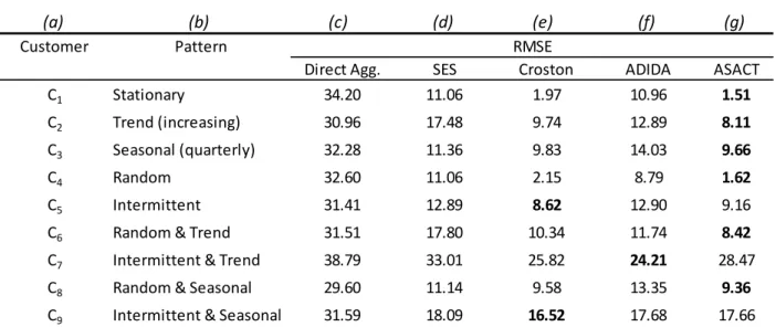
Table 4-2: RMSE for Delivery Type 2 (D2) ... 40
Table 4-3: Error Measures for Delivery Type 1 (D1) ... 41
Table 4-4: Error Measures for Delivery type 2 (D2) ... 41
Table 5-1: Segmentation Results... 63
Table 5-2: Summary of Behavior Patterns ... 78
Table 6-1: Forecast Evaluations ... 102
Table 7-1: Variables (sample shown for illustration) ... 115
LIST OF FIGURES
Figure 2-1: Levels of SCM Collaboration (Holweg et al., 2005) ... 6
Figure 2-2 : Croston Method ... 11
Figure 2-3: Example of DTW ... 13
Figure 3-1: Outline of Research ... 18
Figure 3-2: Overview of Context of Case Study ... 20
Figure 4-1: Traditional Method: Conversion to Time-series ... 31
Figure 4-2: Proposed Method: Conversion to Time-series ... 32
Figure 4-3: Directly Aggregated Data ... 34
Figure 4-4: SES ... 35
Figure 4-5: Croston’s Method ... 36
Figure 4-6: ADIDA Method ... 36
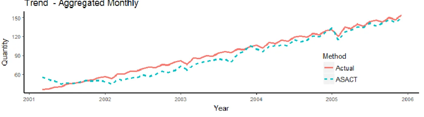
Figure 4-7: ASACT Method ... 37
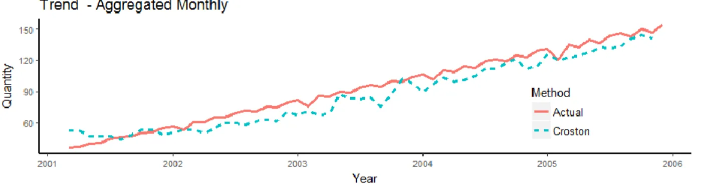
Figure 4-8: Comparitive Resuts for Customer C3 Data Conversions ... 38
Figure 5-1: Segmentation Strategies ... 49
Figure 5-2: Similar Objects with Temporal Shifted Patterns ... 52
Figure 5-3: Example of DTW ... 53
Figure 5-4: Dendrogram of Hierarchical Clustering Results ... 55
Figure 5-5: Methodology ... 57
Figure 5-6: Synthetic Data Aggregated ... 61
Figure 5-7: Expected Clusters in Synthetic Data ... 62
Figure 5-8: DTW with Normalized Data ... 64
Figure 5-9: Industrial Dataset ... 65
Figure 5-11: Cluster Evaluation ... 69
Figure 5-12: Dedrogram of Industrial Data ... 70
Figure 5-13: Proposed Segmentation Method, 8 Clusters ... 71
Figure 5-14: Traditional Segmentation Method, 8 Clusters ... 72
Figure 5-15: Proposed Segmentation Method, 24 Clusters ... 73
Figure 5-16: Traditional Segmentation Method, 24 Clusters ... 74
Figure 5-17: Data Smoothed with Croston’s Method ... 76
Figure 6-1: Proposed Method ... 90
Figure 6-2: Comparison of Methods ... 92
Figure 6-3: Original Customer Data ... 93
Figure 6-4: Outlier Detection & Removal ... 94
Figure 6-5: Cluster Evaluation ... 95
Figure 6-6: Proposed Method Segments ... 96
Figure 6-7: Segment Forecasts ... 97
Figure 6-8: Data for Top-Down Forecast ... 98
Figure 6-9: Top-Down Forecast ... 99
Figure 6-10: Attribute-Based Segments ... 100
Figure 6-11: Attribute-based Segment Forecasts ... 101
Figure 7-1: Methodology Overview ... 109
Figure 7-2: Data Preprocessing ... 111
Figure 7-3: Behavior-Based Segmentation ... 112
Figure 7-4: Behavior-based Segmentation ... 113
Figure 7-5: Step II – Variable Expansion ... 114
LIST OF SYMBOLS AND ABBREVIATIONS
α Alpha (smoothing coefficient)
ADIDA Aggregate, Disaggregate Intermittent Demand Approach
AL Air Liquide
ANN Artificial Neural Networks
ARIMA Auto Regressive Integrated Moving Average
ARIMAX Auto Regressive Integrated Moving Average (extended) ASACT Aggregate, Smooth, Aggregate, Convert to Time-series CCor Cross Correlation
CFPR Continuous Forecasting, Planning & Replenishment CR Continuous Replenishment
DTW Dynamic Time Warping
GIS Geographical Information Systems HAC Hierarchical Agglomerative Clustering
K Number of Clusters
Lin Liquid Nitrogen
Lox Liquid Oxygen
MAE Mean Absolute Error MPE Mean Percent Error
MAPE Mean Absolute Percent Error
ME Mean Error
RFM Recency, Frequency, Monetary RMSE Root Mean Squared Error
SCM Supply chain management SES Simple Exponential Smoothing SOM Self-Organizing Maps
UCM Unobserved Component Models VMI Vendor Managed Inventory
LIST OF APPENDICES
CHAPTER 1
INTRODUCTION
During the industrial revolution, manufacturing firms were vertically integrated; they acquired raw materials, produced their products, and delivered to their customers. Firms such as Ford Motor Company purchased timber, iron ore, and rubber, and relied on their own internal resources to transform, fabricate, and assemble finished products, often in one large location such as Ford’s Rouge River plant (Ford, 2017). While vertical integration was efficient due to centralized control of quality and production it also led to large, inflexible organizations that were slow to change and unable to leverage emerging technologies and alternate sources of labor (Lummus & Vokurka, 1999). Emergent technologies including pallets, forklift trucks, and standard-sized shipping containers enabled more efficient movement of products which allowed the distribution of production activities. Meanwhile, advances in telecommunications and reduction in cultural barriers made it possible for firms from different regions and nations to collaborate. Rather than the traditional vertical integration, firms could now look externally for their material and production requirements. Production de-integration led to the evolution of modern day supply chain management (SCM) (Lummus & Vokurka, 1999). As firms became more and more specialized in their core activities, they began to find benefit from establishing collaborative relationships with firms whose specializations were compatible. The traditional between-firm competition began to transform to a new between-supply-chain competition (Christopher, 2000). In its most basic definition, supply chains (SC) create value by transforming and transporting goods and services that satisfy the demand requirements of downstream partners (Janvier-James, 2012). This definition omits that the success of a SC depends on its ability to leverage strengths and opportunities among a variety of partners in various locations. The successful SC quickly transforms itself to include or remove partners as necessary to suit the products being produced and the marketplace in which it competes. Managing the SC therefore requires an accurate understanding of the product requirements at all levels of the chain (Carbonneau, Laframboise, & Vahidov, 2008); understanding requirements of SC partners is therefore highly dependent on information sharing between partners. The concept of understanding SC requirements, also referred to as demand forecasting, is foundational to our research.
In their seminal paper, Angulo, Nachtmann, and Waller (2004) state that collaborative information sharing was prerequisite for establishing a successful SC, especially in a vendor managed inventory
(VMI) arrangement where the supplier is responsible for managing its customers’ inventory. Subsequent research, however, found that in some VMI arrangements, the SC partners cannot or will not share information (Holweg, Disney, Holmström, & Småros, 2005). Communication technologies between SC partners can be incompatible or non-existent leading to physical barriers to communication (Hernández, Mula, Poler, & Lyons, 2014). Concern of risk, or lack of trust, confidentiality agreements, antitrust laws, and cost of information can also form a barrier to information sharing (Angulo et al., 2004; Kembro & Näslund, 2014). When collaborative information is not available, the supplier must look to other information to understand its SC requirements.
In the absence of external, down-stream SC data, a supplier normally has its own delivery records. In a VMI arrangement where exclusive, long-term supply contracts exist, the delivery records can be expected to provide a good indication of the customers’ consumption behavior. In practice, delivery records are poorly suited for predicting future demand requirements due to the non-linear relationship between delivery transactions and consumption.
Our research has revealed several challenges when attempting to interpret the information gleaned from delivery records. Delivery records reflect more than just the customers’ consumption behaviors. Logistics decisions, such as timing, frequency, and volume of deliveries are reflected in the delivery records; these decisions are not driven by the customer. Moreover, it is well established that as a supply chain decision point moves upstream from the point of consumption, the bullwhip effect increases (Forrester, 1958). Delivery data in its raw form contains a level of noise sufficiently high as to preclude detection of behavior patterns. A method to extract the consumption behavior information from the noisy data is necessary. A second challenge revealed is how to manage predictions for a large population of customers. Aggregating all production requirements together presents a high-level view of the organization, but little knowledge is revealed regarding consumption behavior. Lastly, even when predictions are made at an aggregated level, a method to apply the predictions at the customer level is lacking. In this research, we propose a method for developing customer level forecasts from a large, noisy dataset.
This research has provided important methodological, scientific and practical contributions. In the methodology, we show how a complex problem can be solved through the combination and reapplication of existing tools and methods. The scientific contribution is a solution to solving a
complex business problem where a large stochastic data set is used to generate useful forecast information. And finally, the practical contribution is a tool that can be applied in the case study domain or other similar domains where long-range forecasts are needed, and the available data is limited.
Chapter 2 presents the state of the art relating to relevant areas of SC management and data analytics. Chapter 3 presents our research approach, explains the case study used for the research, and describes the detailed structure of the thesis. Chapters 4 through 7 are the sequential components of the research; these components have been submitted individually to peer reviewed journals for consideration and publication. Discussions, conclusions, and recommendations are offered in Chapters 8 and 9.
CHAPTER 2
CRITICAL LITERATURE REVIEW
2.1
Introduction
The research objective is to develop a method to forecast a SC’s demand requirements based on limited historical data. An accurate forecast will aid the planning of the firm’s resources and save money through increased efficiency. This research problem originates from a real industrial situation, it begins with a real dataset and concludes with a detailed methodology that permits to extract information that can help a firm to understand its SC requirements. The solution to the research problem involves several different steps that relate to different fields of research. SCM is an extremely broad field with many subordinate areas of research. In Section 2.2, we review those SC areas that are relevant to our research to establish context and highlight relevant gaps. In addition to understanding the relevant SC topics, it is also important to understand how the large and noisy data can be managed. Section 2.3 reviews the relevant data analytics.
Regarding VMI, the literature is unanimous in opinion that collaborative information sharing is beneficial, but they also acknowledge that other data must sometimes be substituted, and that that data may be corrupted or noisy due to aggregation and bullwhip effects. There is a gap in the literature as to how to address the noise in the data and make it useful for analysis. We address this gap in chapter 4 which proposes a method to substitute delivery data when consumption data is not available.
Market segmentation is the second step in our proposed method. The literature contains extensive information regarding segmenting the market based on a set of descriptive variables. There is acknowledgement that the accepted strategies do not always produce clusters with homogeneous behavior patterns, but it is not extensively address. Further, little research has been undertaken to develop methods to test cluster validity. The literature does not address how to establish segments when descriptive variables are not available. We address these gaps with our proposed method that establishes market segments based on demonstrated past behavior. This method, which relies on the data smoothed by the method in chapter 4 is described in chapter 5.
The literature on market segmentation all focusses on combining a population into segments to facilitate analysis such as forecasting. There is little guidance on how to de-segment and apply
those subsequent analyses to the individual customers. We proposed a method for that in chapter 6 and evaluate its performance.
Finally, in attempt to address the gap of a method to validate market segmentation results, we propose a method that establishes segments based on demonstrated behavior and then test whether descriptive attributes can achieve similar segmentation results. This method and its results are presented in chapter 7.
2.2
Supply Chain Management
Supply chain management (SCM) emerged when firms recognized that they are no longer able to operate in a vertically integrated structure. Interest in SCM has steadily increased since the 1980’s when firms began to recognize the benefits to between-firm collaborations (Lummus & Vokurka, 1999). There have been many attempts to provide a detailed and encompassing definition of SCM (Cooper & Ellram, 1993; Janvier-James, 2012; Lummus & Vokurka, 1999), however, we prefer a simplified definition that captures the most important components while avoiding the constraints of excessive description and details, as follows: “SCM is the management of the flow of products (or services), money, and information among collaborating firms who move and process the products from raw materials through to the finished goods that are provided to the consumer.” The first two components, products and money, are universally measured and management of them follows well established practices. The third component, information, is not easily quantified and management of its flow can be subjective and constrained (Hernández et al., 2014). Management of information within a supply chain is a key component of understanding SC requirements. Traditional SCM follows push / pull models (Chopra & Meindl, 2007). In “push” SCM, the supplier produces its products and then makes them available to the down-stream members of the supply chain, often placing finished goods into inventory where it awaits purchase from the consumer. In “pull” SCM, the downstream supply chain member, or consumer, determines its needs and places an order with the upstream supply chain member. The push / pull models were robust strategies in that they did not rely heavily on the information component of SCM; firms produced their products when they experienced a trigger (Chopra & Meindl, 2007). In the 1990s, supply chain collaboration began to emerge in several forms, including vendor managed inventory
(VMI); collaborative forecasting, planning and replenishment (CFPR); and continuous replenishment (CR) (Holweg et al., 2005).
2.2.1 Supply Chain Collaboration
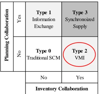
SC partners can collaborate at many different levels including product design, promotions, inventory management, forecast planning, and risk management (Holweg et al., 2005). Since this research is focused on demand forecasting, we will consider only collaboration of inventory management and forecast planning. Holweg (2005) categorized levels of collaboration according to Figure 2.1. When neither planning nor inventory information is shared (Type 0), collaboration does not exist. With Type 1 collaboration, information is shared, and the firms use it to their mutual benefits. With Type 3 collaboration, product flow is synchronized by sharing information about inventory and planning. Type 2 collaboration, VMI, can be complex. In a VMI arrangement, several types of information may be shared between firms. Point-of-sale data, promotion planning, and inventory level information are beneficial for understanding the expected demand requirements. Regardless of how information is shared, the key feature of VMI is that responsibility for inventory management moves upstream to the supplier. The critical point here is that while planning information is beneficial, it is not necessarily shared; critical information from the point of consumption may not be visible to the supplier.
Figure 2-1: Levels of SCM Collaboration (Holweg et al., 2005)
Y es Type 1 Information Exchange Type 3 Synchronoized Supply
No Traditional SCMType 0 Type 2 VMI
No Yes P lan n in g C ol lab or at ion Inventory Collaboration
Research has shown that VMI strategies are effective at increasing SC efficiency, reducing overall costs in the SC, and increasing SC competitiveness (Achabal, McIntyre, Smith, & Kalyanam, 2000; Jung, Chang, Sim, & Park, 2005). Despite a direct link between SC performance and information sharing (Forslund & Jonsson, 2007), SC partners are sometimes unwilling or unable to share useful forecasting information (Holweg et al., 2005; Kembro & Näslund, 2014). In VMI, the responsibility for forecasting ultimately lies with the supplier However, research has shown that supply chain performance can be improved when the information is collaboratively generated through arrangements such as collaborative planning, forecasting, and replenishment (CPFR) (Ramanathan & Gunasekaran, 2014). Ideally, the supplier in a VMI strategy has access to downstream information sources including consumption rates, inventory levels, and forecasts (Achabal et al., 2000).
In a VMI arrangement where downstream forecast information does not exist, the supplier must develop a forecast with other information, typically extracted from historical data or use qualitative information.
2.2.2 Supply Chain Information Sources
VMI requires a source of demand information that is available and timely (Angulo et al., 2004), ideally recorded at the point of consumption. Point of consumption information is not always available, downstream SC partners may be unwilling to share information due to confidentiality, trust, or regulatory concerns. Collecting and transmitting data may be costly or inconvenient, or the amount of data may be too large to process due to high number of customers and transaction events (Holweg et al., 2005).
When consumption-level data is not available, an upstream data source such as delivery records must be used. The information contained in upstream data may be diminished due to aggregation of individual transactions and temporal aggregation; the delivery record becomes a summary of all transactions that occurred since the previous delivery. Moving the data acquisition point upstream has the additional problem of induction of noise due to the bullwhip effect (Biswas & Sen, 2016; Forrester, 1958). Using upstream data for demand forecasting may exasperate the noise problem since the bullwhip effect tends to increase as the data gathering point moves upstream from the point of consumption (F. Chen, Drezner, Ryan, & Simchi-Levi, 2000). In their seminal paper, Lee, Padmanabhan, and Whang (1997) provide a more detailed explanation of the causes of the bullwhip
effect including demand signal processing, order batching, price fluctuation, and rationing. Lastly, when deliveries occur on irregular time intervals and consist of irregular quantities, the resulting data when aggregated into temporal bins can appear lumpy, irregular, and intermittent (Petropoulos, Kourentzes, & Nikolopoulos, 2016), making the data difficult to work with. Despite that delivery records may be directly linked to consumption requirements; the associated noise can make them extremely difficult to work with.
2.2.3 Market Segmentation
When attempting to understand the SC requirements of a large customer population, industry and academics alike often resort to dividing the population into groups and then analyzing the groups instead of individuals (Wedel & Kamakura, 2012). A common term for this grouping is “market segmentation”. Smith (1956) was one of the first to discuss the benefits of market segmentation in his seminal paper on marketing strategies, although he proposed that it should be executed through trial and error. A more advanced segmentation strategy was proposed in the 1970s where determinant attributes were scored to determine segment membership (Anderson, Cox, & Cooper, 1976). The determinant attributes were customers’ responses to a series of questions; the results were subject to bias by the selection and scoring of the questions. Researchers in the 1990s were observing that the outcomes of segmentation analysis were not necessarily resulting in homogeneous clusters (Dibb & Simkin, 2001). Although the literature contains some research on methods for validating market segmentation (Huang, Cheung, & Ng, 2001), the topic has not been extensively explored. Despite some criticism, and limited research on methods to validate it, market segmentation is widely accepted in industry and academia (Rigby & Bilodeau, 2015).
2.3
Data Analytics
Data mining emerged as a popular field of research in the late 1990s (Choudhary, Harding, & Tiwari, 2008), it has since been applied in many areas of research including SCM. Data mining has many descriptors such as “big data analytics”, “data mining”, “data analytics”, “data science”, “knowledge discovery from databases”, and many others including combinations of the ones listed here (Kantardzic, 2011; Manyika et al., 2011; Provost & Fawcett, 2013; G. Wang, Gunasekaran, Ngai, & Papadopoulos, 2016). Regardless of the descriptor used, the common theme is a convergence of several phenomena, including: ever expanding sources of data, powerful and
readily available computers, efficient algorithms, and recognition of data analytics as a competitive advantage for business. “The convergence of these phenomena has given rise to the increasing widespread business application of data science principles and data-mining techniques. (Provost & Fawcett, 2013). In this research, we are interested in a combination of data mining tools that enable the progression from a large and noisy raw dataset to predictions that are manageable and usable in industry. More specifically, we are interested in data preprocessing, clustering, predictions, and evaluation. In some instances, we are fortunate that the necessary tools exist and may be incorporated into our framework. In other instances, we must develop new tools or apply existing tools in ways that they have not previously been tested. We discuss the relevant data analytic topics in the following sections.
2.3.1 Data Preprocessing
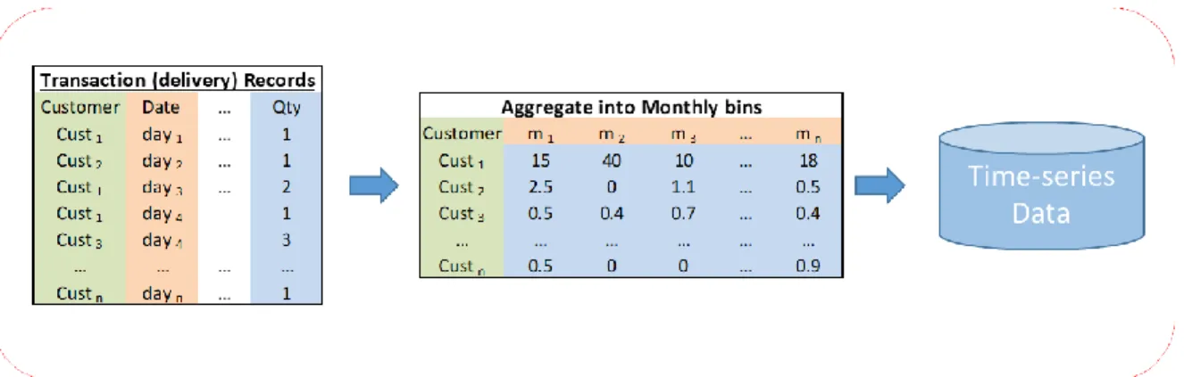
The first thing a data analyst must do when preparing to work on a new problem or with a new set of data is to prepare the data; a process known as data preprocessing or colloquially as data wrangling (Wickham, 2014). The important information contained in real datasets can be shielded or distorted by outliers, missing data points, or irrelevant data (Kantardzic, 2011). Additionally, the structure of the raw data may be incompatible with the intended analysis (Léger, Pellerin, & Babin, 2011). The data analysis must therefore expend considerable effort preprocessing the data to remove unwanted data, fill in missing data, and translate the data into a format that suits. Transaction histories, such as delivery records are sometimes used when actual consumption data is unavailable, however, transaction records do not have a linear relationship to consumption behavior and can be particularly challenging due to irregular occurrence of transactions, errors and omissions in data recording, and the introduction of unknown influences such as the bull whip effect. This type of data requires careful transformation.
Transaction records normally contain a variety of data, but most importantly, date and quantity. The data is easily aggregated into temporal bins to form time-series; a format necessary for subsequent prediction analysis. The resulting time-series, however, is subject to intermittency if the temporal bin size is greater than delivery frequency (Kourentzes, 2014). Intermittent time-series are undesirable due to their difficulty to forecast (Kayacan, Ulutas, & Kaynak, 2010).
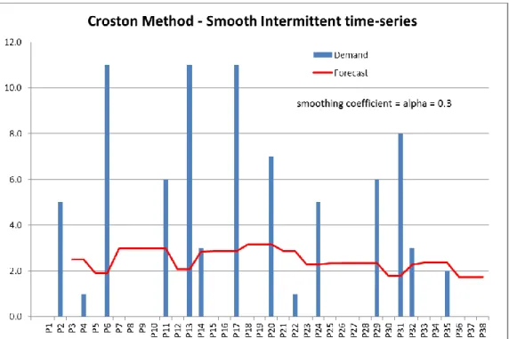
The literature contains several methods for resolving intermittency in time-series; the most famous being Croston’s method (Croston, 1972) which updates only when transactions occur rather than allowing zero-activity periods to degrade the prediction as is the case with simple methods such as exponential smoothing and moving average. Croston’s method is shown in formulae 2.1, 2.2, and 2.3:
𝑦̂𝑡 = 𝑍̂𝑡/𝑋̂𝑡 (2.1)
where 𝑍̂𝑡 is the SES forecast for the non-zero periods and 𝑋̂𝑡is the forecast for the number of inter-demand intervals. Both the inter-demand size and the intervals use SES per formulae 3 & 4:
𝑍̂𝑡= α𝑧𝑦𝑡+ (1 − α𝑧)𝑦̂𝑡 (2.2)
𝑋̂𝑡 = α𝑥𝑥𝑡+ (1 − α𝑥)𝑥̂𝑡 (2.3)
where yt is the non-zero demand at time t and xt is the number of non-zero intervals.
Despite corrections and criticism (Rao, 1973; Syntetos & Boylan, 2005; Willemain, Smart, & Schwarz, 2004), the Croston method remains a standard for handling intermittent time-series (Prestwich, Tarim, Rossi, & Hnich, 2014). Figure 2.1 illustrates the application of Croston method on a simple dataset. In the example, intermittent demand (represented by blue bars) is smoothed using formulae 2.1, 2.2, and 2.3 and alpha set at 0.3. The resulting data (represented by the red line) offers a simplified interpretation of the overall demand.
Figure 2-2 : Croston Method
A contemporary approach known as the “aggregate-disaggregate intermittent demand approach” (ADIDA) (Nikolopoulos, Syntetos, Boylan, Petropoulos, & Assimakopoulos, 2011) has gained acceptance in the literature (Kourentzes, 2014; Petropoulos et al., 2016) despite that fact that ADIDA is actually very similar to applying a simple three-period moving average. A significant improvement over Croston’s method is not found in the literature. In our research, we propose a new adaptation to Croston’s method.
2.3.2 Cluster Analysis
There are several methods for segmenting a population of customers. Simplistic segmentation based on geographic location or customers’ industry type is sometimes used since it is relatively easy. However, the demand characteristics within these segments may be very different and therefore this is not a suitable method (Shapiro, 2007). More advanced segmentation methods are categorized as partitional, hierarchical, density-based, grid-based and model-based (Han & Kamber, 2006). Of these, the most common are hierarchical and partitional (Ahmadi Javid & Azad, 2010; Chakraborty, 2013). Partitional clustering is suitable for handling large data sets due to low computational costs. Applying data mining tools to customer segmentation was a natural progression and many methods have been tested.
By far, the most common data mining method used for clustering is the K-means algorithm, for examples see (Anil K. Jain, 2010; Krieger & Green, 1996; Kuo, Ho, & Hu, 2002). K-means is not a new technique, appearing in Fisher (1958) and further developed by MacQueen (1967). With K-means, a set of N data point are grouped into K clusters with the mean of each cluster becoming its identifying location. K-means, however, relies on Euclidean measurement and it only valid where direct, point-to-point comparisons can be made. Despite its frequent use, K-means has failings due to it ignores natural cluster pattern and rigidly assigns points to individual groups (MacKay, 2003).
An alternative clustering strategy to K-means is Artificial Neural Networks (ANN) and the related Kohonen Self-Organizing Maps (SOM) (Altintas & Trick, 2014). SOM was formally developed by Kohonen as un unsupervised alternative to traditional ANNs (Kohonen, 1990). Unlike K-means where the number of clusters must be pre-defined, ANNs are unsupervised; the number of clusters is part of the ANN’s output.
Several variants of both K-means and ANNs have been developed to overcome some of their failings. These include the addition of fuzzy logic to avoid the rigid assignment of points to clusters (MacKay, 2003). Fuzzy logic allows the identification of groups with similar attributes (Barajas & Agard, 2014) and when combined with partitional clustering it allows flexibility of assigning points proportionally to more than one cluster. The variants are titled with various names that describe their content, such as soft K-means, fuzzy K-means, and fuzzy ANNs.
Hierarchical clustering algorithms are a family of unsupervised algorithms that build clusters in a progressive manner. Divisive hierarchical clustering begins with all members together and progressively divides them into separate clusters until either all clusters have a membership of one, or until the algorithm reaches a pre-defined stopping point. Conversely, hierarchical agglomerative clustering (HAC) builds clusters from bottom up, it begins by assigning one member to a single clusters and then assigning each new member to an existing cluster or a new cluster (Kantardzic, 2011). The results of hierarchical clustering are displayed in a dendrogram.
When identifying clusters based on historical data, such as delivery records, the data is normally formatted into time-series. K-means clustering uses Euclidean distance which is a point-to-point measurement. Two customers with nearly identical consumption behavior will be assessed incorrectly by K-means if their deliveries occur on different days or different frequencies; a more
flexible algorithm is needed. Dynamic time warping (DTW) was initially developed for use in speech recognition, but researchers soon discovered its usefulness in comparing time-series data (Berndt & Clifford, 1994). Unlike Euclidean distance which only assesses directly aligned point, DTW is an elastic measure that is able shift the pairing of points, as illustrated in Figure 2.2, and makes a better comparison between pairs of time-series. Subsequent research supports Berndt and Clifford’s findings that DTW performs well for comparing pairs of time-series (Keogh & Ratanamahatana, 2005). DTW was initially criticized as being computationally expensive, but improvements to its algorithms and increased computer speeds have resolved those concerns to the point where they are no longer a consideration (Izakian, Pedrycz, & Jamal, 2015; Ratanamahatana & Keogh, 2005). DTW is widely accepted as an effective tool for comparing time-series (Mueen & Keogh, 2016).
Figure 2-3: Example of DTW
2.3.3 Prediction Models
Forecasting methods are categorized as qualitative and quantitative (Chase Jr., 2013; Hoshmand, 2010; Moon, 2013). While qualitative methods are frequently used, either as a single method or in combination with other methods, they lack the rigor of quantitative methods (Hoshmand, 2010). Qualitative methods that specifically focus on forecasting do not appear in the literature; rather, the methods are based on general qualitative decision-making theory. The most common qualitative
decision making practices, as applied to forecasting, are Delphi method, jury of executive opinion, sales force composite, focus groups, and panel discussions (Hoshmand, 2010). Despite the weaknesses of qualitative methods, they are essential when historical data and/or resources to develop qualitative forecasts are absent. A major distinction between qualitative and quantitative methods is that while quantitative methods all strictly rely on past event, qualitative methods incorporate forward-looking information.
In contrast to the lack of specific qualitative forecasting methods, quantitative forecasting methods appear frequently in the literature. Makridakis, Wheelwright & Hyndman (2008) list the most common methods as time series decomposition, exponential smoothing (Brown, 1956), regression, and ARIMA (Box & Jenkins, 1962). These and other qualitative methods can be sub-classified into time series methods, causal methods, machine learning methods, and hybrid methods.
Time series methods (including naïve, moving average, exponential smoothing, decomposition, and ARIMA) are built on the premise that “future sales will mimic the pattern (s) of past sales” (Chase Jr., 2013, p. 84). If demand patterns can be detected and accurately modeled, these techniques can be used to generate reasonable forecast accuracy. Time series methods are suitable for harvest brands that have sufficient historical data and steady demand (Chase Jr., 2013).
Time-series that are based on economic data such as sales histories or delivery records are typically non-stationary, so simple models such as naïve and moving average sometimes do not do a good job of representing demand (Phillips & Durlauf, 1986). Adjusting or accounting for non-stationarity can be accomplished by decomposing the information into separate components of trend, seasonality, cycle, autocorrelation, and random error (F. Robert Jacobs, Berry, Whybark, & Vollmann, 2011). Once the time series is represented by its components, it can be de-seasonalized, de-cycled, and de-trended. The resulting pattern can then be modeled by simple methods. Each method utilizes a different level of complexity and decomposition, from the very simple naïve to the more complex ARIMA. However, more complex models do not necessarily produce more accurate results. In fact, the literature generally promotes the rule of using the simplest method that produces actionable results (Clemen, 1989; F. Robert Jacobs et al., 2011; Makridakis, 1989; Maté, 2011).
Causal methods (including simple & multiple regression, ARIMAX, and Unobserved Component Models (UCM) (Harvey, 1989) are based on the assumption that demand is directly related to other
internal or external variables (Chase Jr., 2013). Regression models quantify the correlation between the dependent variable (demand) and one or more independent variables (internal and/or external variables). ARIMAX and UCM both expand on the regression concept by adding features of time series analysis into the models (Chase Jr., 2013; Harvey, Ruiz, & Sentana, 1989). A criticism of causal methods is that they require the forecaster to accurately determine the weighting of the independent variables.
Machine learning methods (including neural networks, recurrent neural networks, and support vector machines) are the newest quantitative methods to be employed for forecasting (Carbonneau et al., 2008). As with time series methods, the machine learning methods are used to detect patterns in past demand behavior from which a forecast can be generated (Azadeh, Ghaderi, & Sohrabkhani, 2007). An advantage to machine learning methods it that unlike causal methods, the contribution (or relevance) of each variable does not have to be predetermined by the forecaster.
Lastly, hybrid methods have been proposed to combine the best features of multiple methods. Unlike combination forecasts that combine the results of different forecast methods (Bates & Granger, 1969), the hybrid forecast method combines the technique of different methods to create a new method. Aburto and Weber (2007) proposed a hybrid method that combines ARIMA and Artificial Neural Networks (ANNs). This appears to be a logical choice considering that ARIMA is widely accepted as an accurate forecasting method and ANNs are gaining recognition in the field. In their research, Aburto and Weber (2007) found that the hybrid model performed better than the baseline Naïve forecast and the ARIMA model.
2.3.4 Evaluation
Market segmentation is the business equivalent to cluster analysis in statistical and data mining sciences. The two differ in how the results of the process are evaluated. There are many examples in the literature for evaluating clusters through various measures of inter-cluster homogeneity and intra-cluster heterogeneity (Ding, Trajcevski, Scheuermann, Wang, & Keogh, 2008; Liao, 2005; X. Wang et al., 2013). Mathematical evaluation presumes that the variables used to calculate the results are meaningful measures. A different approach for cluster evaluation is to conduct a subjective visual assessment of a graph of the results. Visual assessment holds some merit due to human’s innate ability to recognize patterns (Chellappa, Wilson, & Sirohey, 1995), however when
working with big data, it can be impractical to graph the data (Hung & Tsai, 2008). A visual evaluation also lacks a structured recording of how good or bad one result is over another.
In forecasting, a widespread practice is to divide the data into training and testing datasets. The training data is used to build the forecast model and then the test data serves as a known-truth against which the model is tested. In market segmentation, there is usually no known-truth as there is no way to predetermine which clusters a member should belong. We propose a new method in Chapter 7 where the market is established based on historical consumption behavior and then segmentation strategies are tested to see if they can correctly assign segment membership.
CHAPTER 3
RESEARCH APPROACH AND STRUCTURE OF THE
THESIS
3.1
Research Approach
Similar forecasting problems found in the literature tend to offer a single-step solution. For example, in Croston’s seminal paper (Croston, 1972) and in contemporary applications of Croston’s method (Shenstone & Hyndman, 2005), the proposed method resolves intermittent time-series and presents a forecast in the same algorithm. The same single-step strategy was pioneered by Brown (Brown, 1963) with the newly proposed, and now widely used simple exponential smoothing (SES). This research takes a different approach; the solution to the forecasting problem is broken into a series of sequential steps outlined here.
The general problem is how to create an accurate, customer-specific demand forecast based on historical data and in absence of any collaborative input from downstream SC partners. The state of the art shows that many relevant tools exist for this topic, however, attempts to simply choose the best or most suitable tool and apply it are not successful. Our research has shown that a single-step solution is not an effective method for solving this research problem; the sequential application of several different tools is necessary. We leverage existing tools that are demonstrated in the literature, but we sometimes use those tools in ways that have not previously been done. The methodology proposed to solve the overall problem is illustrated in Figure 3.1:
Figure 3-1: Outline of Research
Step 1 – Data preparation: The first challenge is evident when delivery records are aggregated into periodic bins to create time-series. Delivery records are a composite of information that is influenced by a combination of consumption behavior, delivery logistics decisions, inventory management, and the bullwhip effect (Forrester, 1958). The resulting time-series are intermittent, lumpy, and erratic; generating a useful prediction from them is very difficult. A method to smooth the data is necessary. Ideally, the method used to smooth the data should retain the underlying behavior patterns. We offer a method to accomplish this in Chapter 4.
Step 2 – Segment the market based on behavior patterns: The second challenge arises with the analytically intensive task of attempting to maintain individual forecasts for many customers. Although producing many individual forecasts is computationally possible, incorporating them into strategic or tactical business planning requires that they are somehow combined into segments. Forecasting customer segments has been studied in the context of electrical demand (Espinoza, Joye, Belmans, & De Moor, 2005), but it does not appear in the context of forecasting product demand. A reliable strategy for customer segmentation is necessary, it is presented in Chapter 5.
Step 3 – Create segment-level predictions: The third challenge, after the data is smoothed and customers are segmented is how to translate segment-level predictions into individual forecasts. A method to translate the information back to individual forecast is needed and evaluated. This part is presented in Chapter 6.
Step 4 - Translate the predictions to the customer level: The fourth challenge is to quantify and incorporate the effects of exogeneous factors into the forecasts. It is intuitively obvious that some external factors, such as climate, will affect the behavior of some industries, such as agriculture. However, a method to identify, quantify, and apply relevant exogeneous variables to demand forecasts is needed. Also presented in Chapter 6.
Step 5 – Classification based on attributes: The fifth challenge is first to create segments based on demonstrated behavior and then attempt to classify the customers into similar segments based on descriptive attributes. If the descriptive attributes are effective, the resulting clusters should be similar. This part is presented in Chapter 7.
We address these five challenges as individual steps in our research. Some steps are presented as an individual scientific contribution detailed in the papers that make up the body of this dissertation. Although they can stand individually, they are all necessary and propose sequential progressions in forecasting demand from delivery records. Each step is validated on a real case study that is presented in the next section.
3.2
Case Study
The real dataset used in this research was provided by our industrial partner, Air Liquide Americas (AL). AL’s primary products are liquefied oxygen (Lox) and nitrogen (Lin). Point of use inventory of Lox and Lin are managed by AL in a VMI arrangement with the goal of ensuring continuous product availability for its customers while controlling its own internal operations costs (Air Liquide, 2014). In many VMI arrangements, the supplier has access to point of consumption information and is able to make its replenish decisions from that information. However, in AL’s situation the point of consumption information is generally not available and replenish decisions are triggered by low-level sensors on the storage tanks at the customers’ sites.
3.2.1 Industrial Context
AL produces a variety of liquefied and pressurized gasses and which it delivers to its customers via pipeline, tanker truck, and bottles. The context for this research, as illustrated in Figure 3.2 will focus on liquefied Lox and Lin, delivered via specialized tanker trucks to its customers in the continental USA, as illustrated in Fig. 4.
Figure 3-2: Overview of Context of Case Study
AL operates air distillation factories located throughout the continental United States. The factories extract and compress oxygen, nitrogen, and several other elements from atmosphere and store them in liquefied state for distribution to their customers. The liquefied gasses are transported via AL’s specialized fleet of tanker trucks. At the customers’ sites, the liquefied gasses are transferred into storage tanks. AL is responsible for maintaining the customers’ tanks in a VMI arrangement. AL periodically remotely queries the tank level sensors to determine if a replenishment delivery is necessary. Continuous level sensing and recording is possible at some locations, but in practice it is not used for operations decisions; tank levels and point-of-use consumption data is not recorded. Ideally, AL will coordinate delivery schedules so that an entire tanker load will be delivered to a
single customer site. However, partial deliveries are necessary for smaller customers. When partial tanker-load deliveries are necessary, the balance of the load is sometimes delivered to a second customer in effort to increase overall logistics efficiency.
AL’s delivery scheduling is further complicated by its factories using the same distillation systems for more than one element and limited storage capability. Deliveries therefore depend not only on customers’ needs, but also on product availability. Customer requirements, delivery logistics, and product availability all influence the information gathered in the delivery records.
3.2.2 Data Description
AL provided its delivery records for all customers and all products in the continental USA from January 2009 through September 2014. AL did not perform any data cleaning or preprocessing prior to transferring the data to us, although it did remove fields with descriptive customer information to anonymize the data. Liquid nitrogen (Lin) and liquid oxygen (Lox) make up the majority of AL’s product sales and these were retained for study; records for other products were removed from the data. Each delivery event in the data includes delivery date, product quantity, product description, customer number, customer location, AL distribution center location, and an industry identifier number. Prior to cleaning, the 66 months of data contained 1.18 million delivery events and over 8000 unique customers. Considering that the research is focused on identifying and predicting customer behaviors, only customers with consistent and persisting transactions were retained. Infrequent customers, lost customers, and new customers were removed. Also, a very small number of customers with unexplainable quantities or suspected corrupted data were removed. For the data cleaning, infrequent customers are defined as having less than 12 months with deliveries, lost customers have no deliveries in the last year, and new customers have no data during the first two years. After initial data cleaning, approximately 3000 unique customers were retained for the case study. Although more than two thirds of the customers were removed, they represent only 25% of the delivery events; 880,000 of the original 1,118,000 observations are used in the case study.
3.3
Research Methodology
The research objective, as stated in section 2.1, is to develop a method to forecast a SC’s demand requirements based on limited historical data. In the case study, a dataset of delivery records was the only available information. Secondary data sources, such as consumption data, invoice records, purchase contracts, or inventory audits were not available and therefore it was not possible to validate the dataset through any direct comparison. Initial inspection of the data revealed some entries that were obvious errors due to extreme or impossible values. However, deciding the level at which the records could be identified as outliers and removed from the study was subjective. Considering that the research objective did not include maximizing participation in the study, the level for identifying outliers was set low. A secondary data source for auditing the dataset would allow less outlier removal.
The literature review and testing of established forecasting methods did not reveal an existing method to produce a useful forecast from the noisy stochastic dataset. The research methodology was therefore based on a framework of existing tools and methods that were able to incrementally progress toward solution of the problem. Within each step of the framework, decisions such as selecting a smoothing coefficient value or choice of clustering method were necessary. While many tests were conducted to validate these types of decisions, the search was not exhaustive, and the overall framework is not optimized. Rather, the goal here was to demonstrate a working solution that could later be optimized depending on the domain where it is applied.
3.4
Structure of the Thesis
The thesis is presented in nine chapters, as follows:
Chapter 1 is the introduction which presents the research problem and highlights the significance of the solution to the research problem
Chapter 2 presents the state of the art in the relevant topic areas. The state of the art shows how others have managed similar problems. The gap in the research literature is highlighted.