Analyzing Real Cluster Data for Formulating Allocation Algorithms in Cloud Platforms

HAL Id: hal-01094388

https://hal.inria.fr/hal-01094388

Submitted on 19 Jan 2015

HAL is a multi-disciplinary open access

archive for the deposit and dissemination of

sci-entific research documents, whether they are

pub-lished or not. The documents may come from

teaching and research institutions in France or

abroad, or from public or private research centers.

L’archive ouverte pluridisciplinaire HAL, est

destinée au dépôt et à la diffusion de documents

scientifiques de niveau recherche, publiés ou non,

émanant des établissements d’enseignement et de

recherche français ou étrangers, des laboratoires

publics ou privés.

Analyzing Real Cluster Data for Formulating Allocation

Algorithms in Cloud Platforms

Olivier Beaumont, Lionel Eyraud-Dubois, Juan-Angel Lorenzo-Del-Castillo

To cite this version:

Olivier Beaumont, Lionel Eyraud-Dubois, Juan-Angel Lorenzo-Del-Castillo. Analyzing Real Cluster

Data for Formulating Allocation Algorithms in Cloud Platforms. Proceedings of the IEEE 26th

International Symposium on Computer Architecture and High Performance Computing (SBAC-PAD),

Oct 2014, Paris, France. pp.302 - 309, �10.1109/SBAC-PAD.2014.44�. �hal-01094388�

Analyzing Real Cluster Data for Formulating

Allocation Algorithms in Cloud Platforms

Olivier Beaumont, Lionel Eyraud-Dubois and Juan-Angel Lorenzo-del-Castillo

Inria Bordeaux Sud-Ouest. 200 avenue de la Vieille Tour, 33405 Talence, France.

Email: olivier.beaumont@inria.fr, Lionel.Eyraud-Dubois@inria.fr, juan-angel.lorenzo-del-castillo@inria.fr

Abstract—A problem commonly faced in Computer Science research is the lack of real usage data that can be used for the validation of algorithms. This situation is particularly true and crucial in Cloud Computing. The privacy of data managed by commercial Cloud infrastructures, together with their massive scale, make them very uncommon to be available to the research community. Due to their scale, when designing resource allocation algorithms for Cloud infrastructures, many assumptions must be made in order to make the problem tractable.

This paper provides deep analysis of a cluster data trace recently released by Google and focuses on a number of questions which have not been addressed in previous studies. In particular, we describe the characteristics of job resource usage in terms of dynamics (how it varies with time), of correlation between jobs (identify daily and/or weekly patterns), and correlation inside jobs between the different resources (dependence of memory usage on CPU usage). From this analysis, we propose a way to formalize the allocation problem on such platforms, which encompasses most job features from the trace with a small set of parameters.

I. INTRODUCTION

The topic of resource allocation algorithms for Cloud Computing platforms has been the focus of recent interest. In this context, the objective is to allocate a set of services or virtual machines (VMs) on a set of physical machines, so as to optimize resource usage, or ensure strong Quality of Service guarantees, or limit the number of migrations used, among others. On the algorithmic side, several solutions and techniques have been proposed to compute such allocations: many are based on variants of standard Bin Packing algorithms (like First Fit or Best Fit), some are more focused on the dynamic aspect and provide online rules to compute new valid allocations. There is no clear consensus in the community on which aspects of the problem are most important (dynamicity, fault tolerance, multidimensional resources, additional user-supplied constraints, ...), neither on the formal algorithmic models to take such aspects into account.

In this paper, we analyze a cluster usage trace recently released by Google with the goal of answering some of these questions. Some of the characteristics of this trace have already been analyzed in [1]. Our objective in this paper is twofold. Firstly, we aim at finding new characteristics of the trace and to exhibit the main properties of the jobs running on it. Second, we aim at proposing a set of very few parameters that still account for the main characteristics of the trace and may leverage both the generation of realistic random traces and the design of efficient allocation algorithms.

A. The Google Cluster Trace

Google recently released a complete usage trace from one of its production clusters [2]. The workload consists of a massive number of jobs (or services), which can be further divided into tasks, being each task assigned to a single physical machine. The data are collected from 12583 heterogeneous machines, span a time of 29 days and provide exhaustive profiling information –such as the memory and CPU usage of each task– on 5-minute monitoring intervals (called time windows in the rest of this paper). Each job has a priority assigned, being 0 the lowest one and 11 the highest one. Ac-cording to [3], [4], priorities can be grouped in infrastructure (11), monitoring (10), normal production (9), other (2-8) and gratis (free) (0-1). The scheduler generally gives preference to resource demands from higher priority tasks over tasks belonging to lower priority groups, to the point of evicting the latter ones if needed. Let us note that the goal of this paper is not to understand the behavior of the scheduling algorithm used by Google to allocate tasks and jobs, but to concentrate on the general properties of the jobs themselves and how to describe the trace.

The whole trace is split in numerous files with a total size of 186 Gb. These trace files contain thorough information about the platform and the jobs running on it. The main difficulty is related to the size of the database and the time needed to validate any assumption based on these data. In this paper we propose an extraction of the database containing all information about the jobs that we consider as dominant, i.e. jobs that at some instant belong to the minimal set that still accounts for most of the resources usage, and that can be used to test and validate more easily new assumptions.

B. Relevant Features and Important Questions

Based on the trace of the production clusters described in [2], we will in particular concentrate on the following questions :

Static: It has been noticed in [1] that, at a given time step, a small portion of jobs only accounts for most of the usage of the platform (both in terms of CPU usage, memory consumption, number of assigned tasks,...). In this study, we confirm this observation. In particular, we prove that less than 6% of all jobs account for almost 95% of CPU usage and 90% of memory usage. A crucial consequence is that, in this context, it is possible to design efficient and optimized algorithms to allocate these jobs, contrarily to what is often assumed in the literature, while possibly relying on basic on-line linear complexity heuristics to schedule the huge number of very small remaining jobs. We also provide a detailed analysis of

the class of priorities of these jobs and of the number of tasks they involve.

Dynamic: In the context of the design of efficient algorithms, the dynamics of jobs have also to be considered. Indeed, as already stated, we observe statically (at any time stamp) that the number of dominant jobs necessary to account for most of the platform usage is relatively small. Related to the dynamics of the system, we will consider the following additional questions: does the set of dominant jobs vary over time or is it relatively stable? What is the distribution of lifespan of dominant jobs? How much of the overall CPU usage does the set of stable dominant jobs account for? Does the usage (memory, CPU, tasks) of dominant stable jobs vary over time and, if it is the case, do they exhibit specific (hourly, daily, weekly) patterns? In the context of resource allocation mechanisms, this information is crucial in order to determine, even for the small set of dominant jobs, what can be done statically for a long period and what needs to be recomputed at each time step.

Advanced features of the jobs: As stated above, a priori, each job comes with a given number of tasks (or with an overall demand in the case of web services for instance) in terms of CPU, memory, disk, bandwidth... This leads to multi-dimensional packing problems that are notoriously difficult to solve, even for relatively small instances (a few hundreds of items). Nevertheless, multi-dimensional packing problem are greatly simplified if there are correlations between the different dimensions. In this paper, we will mostly concentrate on CPU-Memory correlation. We will prove (by depicting for all the tasks from dominant jobs, at all time stamps, their memory and CPU footprints) that for a large fraction of the jobs, the CPU usage varies with time and from task to task but that the memory usage is (almost) independent of the CPU usage. More precisely, we will classify the jobs into a few categories. Fault Tolerance Issues: In such a large platform (typically involving more than 10k nodes), failures are likely to happen. In the case when a SLA has been established between the provider and the client, replication or checkpointing strategies have to be designed in order to cope with failures. In this paper, we will concentrate on the following questions: what is the actual frequency of failures on such large scale production cluster? Are failures heavily correlated (a relatively large number of nodes fail simultaneously) or mostly independent? Again, these observations can be later used in order to validate failure models or to precisely quantify the qualities and limits of a model.

The rest of this paper is organized as follows. Section II presents the related work and clarifies our contribution. In Sec-tion III, we define the set of dominant jobs which account for most of the resource usage and provide a simple description. In Section IV, we analyze the static properties of the workload of this dominant set of jobs. More dynamic properties following the evolution of jobs over time are considered in Section V. Issues related to failure characterization will be considered in Section VI. Section VII proposes a variety of reasonable simplifying assumptions which can be made when designing allocation algorithms. Concluding remarks are presented in Section VIII. Note that it is impossible to include in this paper all the plots and numerical results and we will present throughout the text a small set of examples spanning all the questions above.

II. RELATED WORK

The trace has been published by Google in [2] and its format described in [3]. A forum to discuss trace-related topics is available in [5]. Several teams have analyzed this trace and the associated workload. Reiss et al. made a general analysis in [1] and [4], paying special attention to the workload heterogeneity and variability of the trace and confirming the need for new cloud resource schedulers and useful guidance for their design. Di et al. [6] used K-means clustering techniques in an attempt to classify the type of applications running in the trace based on their resource utilization. As a previous step, a comparison of these applications with respect to those which typically run on Grids was done in [7]. In [8], Liu and Cho focused on frequency and pattern of machine maintenance events, as well as basic job-and-task-level workload behavior. Garraghan et al. made in [9] a coarse-grain statistical analysis of submission rates, server classification, and wasted resource server utilization due to task failure.

Other teams have used the trace as an input for their simulations or predictions. Di et al. used it in [10] to test fault-tolerance optimization techniques based on a check-pointing/restart mechanism, and in [11] to predict host load using a Bayesian model. Amoretti et al. [12] carried out an experimental evaluation of an application-oriented QoS model. On a different context, job burstiness is used as an input for a queue-based model of an elasticity controller in [13].

All these approaches have always been carried out either without any particular application in mind or just as an input to test simulations. On the contrary, our analysis aims at discriminating those features from the trace that are relevant to define a model which captures the main characteristics of both jobs and machines, that is tractable from an algorithmic point of view (not too many parameters) and that can later be used for random generation of realistic traces.

On the other hand, some work has already been done to analyze the dynamics of resource usage in datacenters. Bobroff et al [14] proposed a dynamic consolidation approach to allocate VMs into physical servers reducing the amount needed to manage SLA violations. They analyze the historical usage data and create an estimated model, based on auto regressive processes, to forecast the probability function of future demand. Gmach et al [15] rely on pattern recognition methods to generate synthetic workloads to represent trends of future behavior. In this paper, we analyze a much larger dataset, which is publicly available, and we analyze both the dynamics and the repartition of resource usage to provide a set of well-justified assumptions for the design of allocation algorithms.

III. DOMINANT JOBS

In this section, we analyze the repartition of resource usage between jobs, and more precisely of those jobs which are crucial when designing efficient allocation algorithms. Following [1], we will prove that at any time step, a small portion of the jobs accounts for a large portion of CPU and memory usage. Therefore, reasonable resource allocation algorithms should concentrate on a careful allocation of these dominant jobs.

Stats Ratios

|D| |D|/Alljobstw Rcpu Rmem

mean 240.9 0.058 0.947 0.890 std 13.8 0.003 0.009 0.008 min 203 0.050 0.905 0.840 25% 232 0.056 0.942 0.886 50% 239 0.058 0.947 0.891 75% 248 0.059 0.953 0.895 max 336 0.082 0.975 0.913

TABLE I: Number of dominant jobs, and ratios of number of jobs, CPU and memory usage w.r.t. all other jobs, per time window.

numTasks totalcpu totalmem

0.0 0.2 0.4 0.6 0.8 1.0 _Priority Gratis Other NormProduction Monitoring Infrastructure

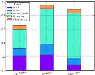
Fig. 1: Average resource usage of dominant jobs stacked by priority class.

As mentioned before, the trace contains monitoring data averaged over 5-minute time windows. From each window to the following one, the number of running jobs will vary to a larger or lower extent, depending on the dynamicity of the trace in that period. Hence, jobs that account for most of resource usage at a time window will not necessarily do it in the next one. We looked for a set of jobs that were representative of the whole trace. We define Di, the set of dominant jobs for a

given time window i, as the smallest set of jobs which account for at least 90% of the CPU usage of this time window. The set of dominant jobs which we consider in this paper is the union of these sets over the whole trace, D=SiDi. This set

D contains 25839 jobs, which is 3.8% of all jobs in the trace. Table I shows the number of alive jobs in D and its resource usage R(D) (CPU and memory) relative to the corresponding values on each time window (tw). The first row shows that, in average, 240.9 jobs (i.e. 5.8% of the jobs running on each tw) account for 94.7% of the overall CPU usage and 89% of the memory usage. This confirms that, even though the overall trace involves a huge number of jobs, it is of interest to concentrate on a very small fraction of them that accounts for most of platform usage at any time. In the rest of the paper we will focus only on these dominant jobs.

The small amount of jobs that comprises the dominant set is a crucial observation when considering the design of resource allocation algorithms. Indeed a quadratic (resp. cubic) complexity resource allocation would be 1000 (resp. 4 · 104

) times faster on this small set of jobs rather than on the whole set, while still optimizing the allocation of the jobs that account for almost all of the CPU usage. It can be noted that these jobs involve a large number of tasks (470 on average, for 49983 the largest one), what explains their overall weight. It is therefore crucial for the algorithms to concentrate on jobs and not on tasks (or virtual machines).

A second observation that can be made is that, for those jobs that account for 90% of the CPU usage, most of the workload is dominated by jobs from particular priority groups. Figure 1 shows three parameters of the trace (number of tasks, total CPU and memory usage) normalized to the total cluster utilization and stacked by priority classes. From this, it can be observed that the set of dominant jobs, which accounts for more than 94% of CPU usage and almost 90% of the overall memory usage, comprises only 65% of the overall number of tasks. The memory and CPU usage bars show that most of jobs belong to the Normal Production priority class. Jobs in that priority class are prevented from being evicted by the cluster scheduler in case of over-allocation of machine resources. The second most important set of jobs are the ones in the Gratis priority class. Gratis priority class jobs are defined as those that incur little internal charging, and therefore can be easily evicted by the cluster scheduler if needed due to over-allocation. Note that, according to the leftmost bar from the figure, the number of tasks from jobs in the Gratis priority class is almost as large as those with Normal Production priority (21% versus 27%, respectively).

IV. WORKLOAD CHARACTERIZATION

In this section, we analyze more precisely the static be-havior of the workload of dominant jobs. We first describe the distribution of total resource usage for jobs in this set, and find that it can be summarized by a lognormal or a mixture of two lognormal distributions. Then, we analyze the relations between memory and CPU usage of individual tasks inside a job. Indeed, in the most general setting, resource allocation is amenable to a multi-dimensional bin packing problem (where the dimensions correspond to CPU, memory, disk,...), that are known to be NP-Complete and hard to approximate (see for instance [16] for the offline case and and [17] for the online case). On the other hand, being able to find simple models relating CPU and memory usage can dramatically reduce the complexity of packing algorithms.

A. Job resource usage

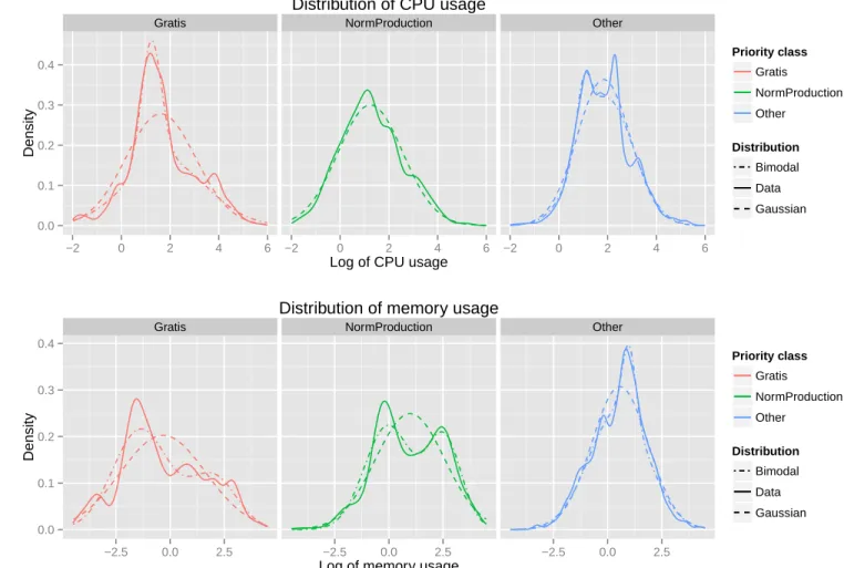
For this analysis, we have computed the mean CPU and memory usage of all jobs in the dominant set, and we have analyzed the behavior of the logarithm of these values. The result is shown on Figure 2, and shows that these distributions can be roughly approximated by a Gaussian distribution, which implies that the actual resource usage can be approximated by a lognormal distribution. However, for more precision, it is possible to model them using a mixture of two lognormal distributions. The parameters of the distributions used are given in Table II. It is interesting to note that although Normal

Gratis NormProduction Other 0.0 0.1 0.2 0.3 0.4 −2 0 2 4 6 −2 0 2 4 6 −2 0 2 4 6

Log of CPU usage

Density Priority class Gratis NormProduction Other Distribution Bimodal Data Gaussian

Distribution of CPU usage

Gratis NormProduction Other

0.0 0.1 0.2 0.3 0.4 −2.5 0.0 2.5 −2.5 0.0 2.5 −2.5 0.0 2.5

Log of memory usage

Density Priority class Gratis NormProduction Other Distribution Bimodal Data Gaussian

Distribution of memory usage

Fig. 2: Usage density distributions of dominant jobs for CPU (top) and memory (bottom).

Classes Gaussian Gaussian mixture

µ σ λ1 µ1 σ1 λ2 µ2 σ2 CPU Production 1.24 1.33 Gratis 1.62 1.43 0.68 1.79 1.68 0.32 1.23 0.41 Other 1.84 1.10 0.11 1.02 0.30 0.89 1.94 1.12 Memory Production 0.98 1.60 0.60 -0.04 1.08 0.40 2.54 0.81 Gratis -0.32 1.97 0.69 -1.36 1.28 0.31 1.98 1.08 Other 0.57 1.30 0.88 0.51 1.37 0.12 0.99 0.31

TABLE II: Parameters of distributions used in Figure 2. For the mixture distributions, λ1and λ2are the weights associated

to the two normal distributions with given µ and σ.

Production jobs account for most of the resource usage in total, individual jobs in the other priority classes (Gratis and Other) use more resource but, since their duration is shorter, fewer of them are alive at any given time.

B. CPU vs Memory Usage

In this section, we will concentrate on memory and CPU dimensions, for which data are available in the trace. Other dimensions (bandwidth, for example) are not provided. In fact, the trace provider strongly advises not to speculate about them. Let us consider the case of a job corresponding to a web service typically handling requests. The memory footprint comes from two different origins. There is first a constant memory footprint that corresponds to the static size of the code being executed. Then, there is a memory footprint that is due to dynamic memory allocations and that is typically expected to be proportional to the number of requests being handled by the task, and therefore to its CPU usage.

In order to find out if there exists any correlation between memory and CPU, we sampled the resource usage of the set of dominant jobs at 20 random timestamps per day, which makes 600 samples along the trace. Note that some of these jobs might never run simultaneously, but we are interested here in the characteristics of each individual job. For each job, we have analyzed simultaneously the memory and CPU usage of each of their individual tasks at all timestamps when this job is alive.

0.00 0.01 0.02 0.03 0.04 0.05 0.06 0.07 cpu (core-sec/sec) 0.00 0.01 0.02 0.03 0.04 0.05 0.06 memory (bytes) (a) 0.000 0.002 0.004 0.006 0.008 0.010 0.012 cpu (core-sec/sec) 0.000 0.001 0.002 0.003 0.004 0.005 0.006 memory (bytes) (b) 0.00 0.01 0.02 0.03 0.04 0.05 0.06 cpu (core-sec/sec) 0.000 0.005 0.010 0.015 0.020 0.025 0.030 memory (bytes) (c) 0.00 0.05 0.10 0.15 0.20 0.25 0.30 0.35 0.40 cpu (core-sec/sec) 0.000 0.001 0.002 0.003 0.004 0.005 0.006 0.007 memory (bytes) (d)

Fig. 3: Dependency of memory usage vs CPU consumption of four different jobs.

with different memory-CPU utilization. So, before the analysis, patterns were clustered into groups using a DBSCAN algo-rithm. DBSCAN uses as a metric distances between nearest points and, therefore, views clusters as areas of high density separated by areas of low density [18]. After this clustering, we performed simple linear regression on each discovered cluster. We used the r-squared value from the linear regression and the coefficient of variation (for each cluster, standard deviation of the distances of all tasks to the regression line, divided by the mean value of the tasks) to decide whether the linear regression was a good approximation for this cluster behavior, and we conservatively rejected as BadlyFitted all jobs in which at least one cluster was not approximated correctly. This selection rejected about half of the considered jobs. For the other half, patterns were classified into Flat or Slope by using a threshold on the range parameter, defined as the ratio between the value estimated by the linear regression for the median CPU usage and for 0 CPU usage.

In Figure 3, each plot corresponds to a job and each dot (cpu,memory) shows the specific usage profile of each job’s task. Each color is associated to a specific cluster. Typical situations are depicted on each plot. The top left figure corresponds to the case where the memory usage is independent of the CPU usage. According to the classification algorithm, this situation occurs in 67% of all the fitted cases. A comparable situation is depicted in the top right figure. In this case, the job comprises two different clusters, and could be considered for resource allocation issues as two different jobs. According to the classification, this situation accounts for 6.5% of the fitted jobs. Therefore, in 72.5% of the cases, it is possible to assume that the memory footprint of a job’s task is independent of their CPU usage. The situation depicted in the bottom left figure corresponds to the case where the memory footprint is affine in the CPU usage, with a non-flat slope (corresponding to the previous case depicted by top

figures). According to our classification, this occurs in 26.5% of the cases. There also exists a certain amount of jobs that does not follow any clear pattern, and which were classified as BadlyFitted. An example is depicted on the bottom right figure. In this case, it seems that the job consists of many sub-jobs, all tasks in each sub-job being assigned the exact same CPU but varying memory.

Nevertheless, we can observe that for an important amount of jobs, and with a very conservative selection, it is possible to model memory usage as an affine function of the CPU usage (2 parameters per job) and that for most of these jobs, it is even possible to model the memory usage as a constant (1 parameter per job). As proven in [19], this assumption strongly simplifies resource allocation problems in Clouds.

V. DYNAMIC FEATURES

A. Dynamics of Dominant Jobs

In this section, we consider the dynamics of the dominant jobs identified earlier. The first question to consider is about the “stability” of this set of dominant jobs: how much does the set of dominant jobs change over time? To provide answers to this question, we have analyzed the distribution of their durations, which is shown on Table III for the three main priority classes. We can see that the Gratis and Other priority classes have similar behavior: most jobs in these classes last for a very short time (half of them last less than 25 minutes), but some last much longer (1% of Gratis jobs last more than 30 hours, 1% of Other jobs last more than 15 hours). However, the Normal Production jobs are much more stable: half of them run for more than 31.7 hours. In fact, about 15.6% of all Normal Production dominant jobs run for the whole trace.

Another interesting question arises when observing the variation of resource usage of jobs: we have noticed that the CPU usage of Normal Production jobs follows interesting periodic patterns. In the following subsection, we analyze how much correlation exists between the CPU usage of individual jobs.

B. CPU usage variation

When considering allocation, it is important to categorize the correlation among jobs to be scheduled and/or already scheduled. Indeed, if a resource provider knows that there is a high probability of having two jobs positively correlated in, say, CPU demand, it will take care to allocate them in

Stats Duration of jobs (min)

Gratis Normal Production Other

mean 186 6.79d 102 std 1653 10d 938 25% 10 170 15 50% 25 31.7h 25 75% 65 6.98d 55 90% 185 29d 120 95% 365 29d 255 99% 30.1h 29d 15.5h

TABLE III: Distribution of job durations in the main priority classes. 29 days is the whole duration of the trace.

02 05 08 11 14 17 20 23 26 29 Day 0 1 2 3 4 5 6 7 Cpu (core-sec/sec)

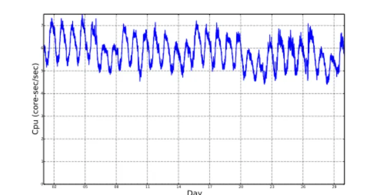
Fig. 4: Example of CPU usage of a long-running, Normal-Production job showing daily and weekly patterns.

different machines to avoid starvation of any of them in the event of a spike of demand. On the other hand, two negatively correlated jobs, allocated together, will allow for a better average utilization of the available resources. To perform this analysis, we have restricted to jobs in the Normal Production class, because jobs in the other priority classes do not last long enough, and thus analyzing correlations and usage patterns does not make sense. Furthermore, considering only one priority class avoids (at least partially) the correlation due to the fact that the platform has finite capacity. Indeed, this finite capacity implies that when the demand of one job increases, it uses more resource, and then another job may end up using less resource (or even get evicted) even if its actual demand did not change.

By looking at individual resource usage of Normal Pro-duction jobs provided an interesting insight in their behavior: all jobs that are long enough present daily and sometimes weekly patterns. This can be seen for example on the Normal Production, dominant job shown in Figure 4. Since any signal is the sum of its Fourier components, it is possible to recreate the pattern of a group of jobs by just providing statistical values about the amplitude ratios between the main components, together with a small number of parameters such as frequency, amplitude and phase of the main components of each job, as well as a given amount of random noise.

We have analyzed the Normal Production, dominant jobs that run during the whole trace. The CPU demand of each job was decomposed into its Fourier series to quantify its main spectral components. After removing the harmonics, we quantified their amplitude, phase, frequency and background noise. Table IV provides the averaged ratios between signal amplitudes and the constant part. We can see that the residual noise is about 6% of the average CPU demand for a large part of the jobs, and this can be used as a threshold: any pattern with an amplitude significantly larger can be identified as a relevant component. Our first observation is that very few jobs exhibit hourly patterns, whereas more than half of the jobs exhibit very strong daily patterns, and two thirds of the job have significant daily patterns. Weekly patterns are not as strong, but they are still significant for about half of the jobs. The long term part of the signal represents variations on a larger time-scale, and we can see that this variation is also significant for many jobs, but it can not be analyzed any further because the duration of

Stats Ratio of amplitude to mean

Hourly Daily W eekly Long term N oise

mean 0.057 0.267 0.148 0.154 0.100 std 0.246 0.232 0.127 0.161 0.154 min 0.001 0.006 0.011 0.001 0.012 25% 0.004 0.052 0.076 0.051 0.036 50% 0.007 0.268 0.106 0.102 0.058 75% 0.009 0.376 0.196 0.196 0.072 max 1.612 1.075 0.669 1.149 0.836

TABLE IV: Ratios amplitude/mean for long-running, dominant jobs.

the trace is only one month.

Another interesting question is how much these patterns are synchronized: if all jobs reach their peak demand at the same time, the stress on the platform and on the resource allocation algorithm is much higher. On the other hand, if the peaks are spread on a large enough timeframe, this provides some slack to the allocation algorithm to provide efficient allocations by co-allocating jobs whose peaks happen at different times. From our observations, jobs which exhibit a weekly pattern have all the same (synchronized) behavior: 5 days of high usage, followed by 2 days of lower usage. About daily patterns, we have analyzed the repartition of the phase for those jobs which exhibit a daily pattern (with an amplitude of at least 10% of the mean).

It appears that for half of the jobs, the phase difference is below 60 degrees, which means that their peaks are within 4 hours of each other. Furthermore, 90% of the jobs exhibit a phase difference below 120 degrees, which means that the peaks are at most 8 hours apart. This shows that the behavior of jobs are clearly correlated by this daily pattern, however there are indeed opportunities for good allocation strategies to make use of this 8 hour difference between the peak times of some jobs.

VI. MACHINE FAILURE CHARACTERIZATION

The Google trace also includes information about machine events, in particular about times when some machines are removed from the system. According to the trace description, these “removed” events can be either machine crashes, or planned maintenance. An usual assumption for modeling fault-tolerance issues is that machines fail independently: the failure of one machine does not change the failure probability of other machines. Another assumption is that the failure probability of machines does not change with time. When both assumptions hold, the number of failures in a given time period is a random variable which follows a Poisson distribution P(λ), where λ is the average number of failures.

# events 0 1 2 3 4 5 6 # time windows 3617 2656 1280 432 168 78 37 # events 7 8 9 10 11 13 14 # time windows 18 11 4 7 5 2 5 # events 15 16 17 18 19 20 23 # time windows 9 1 2 3 7 1 2 # events 25 30 46 47 54 # time windows 3 1 1 1 1

1e−01 1e+01 1e+03

0 1 2 3 4 5 6 7 8 9

Number of events

Number of time windo

ws

Value Actual Expected

Distribution of machine removal events

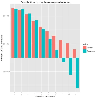
Fig. 5: Actual versus expected distribution of failures

In order to test these assumptions, we have counted the number of removals in all 8351 5-minutes time windows of the trace. The result is shown on the above table, where the average number of removals is 1.07. Since the trace contains information about 12,000 machines, this would represent an (individual) machine failure probability of 10−4 _{in each time}

window. This table shows that in most time windows, the number of removals is rather small, but we can identify 51 time windows with at least 10 removals. Such occurrences are very unlikely under the Poisson distribution: the expected number of such time windows is less than2.10−3_{, which clearly indicates}

that some correlation exists. Of course, planned maintenance events are expected to be correlated, so the existence of such events could easily justify these occurrences, while keeping the independence assumption for ”natural” failures.

For the next step, let us ignore the time windows that we expect to correspond to maintenance sessions, by assuming that all time windows with at least 10 removals are maintenance events. There are 8301 remaining time windows, for which the mean number of events is0.97. Figure 5 shows the actual number of time windows for each number of events, together with the expected value (under a Poisson distribution). This figure shows that time windows with more than 5 failures are still much more present in the trace than what would be expected from a Poisson distribution. This hints at the presence of some correlation on machine failure events, which should be taken into account in a complete model for machine failures. However, a more in-depth analysis would require to be able to differentiate between maintenance and actual failure events and as a first approximation, independent failures with a failure rate of 10−4 _{in each 5 minutes period can be considered as a}

reasonable model.

VII. MODELING THE WORKLOAD

The work presented in previous sections quantifies the type of workload existing in actual datacenters such as Google’s. From this analysis, we provide a set of parameters that allows for creating a reasonable, yet simple, model which can be used as an input of a system (for example, an algorithm) in the context of resource allocation.

There are several decisions that need to be taken during the model generation process. Among them, the number of degrees of freedom allowed. Simply put, which parameters should we use in our model, how many of them, and how much can they vary? Too few parameters will result in a simplistic model that may not reliably reflect the features of the modeled workload. Too many parameters can overfit the model, so it will be more complex without this ensuring at all that it will provide better results. In fact, there is no such thing as a good or bad model, since it depends on the system to which it will be applied. For example, a system whose output is a function of the input memory usage will probably not care about job priorities or CPU usage. However, it might take into account, to a larger or lesser extent, the memory usage distribution and memory periodic patterns.

We believe that for such large datacenters with many tasks, the focus of the allocation system or algorithm should be on whole jobs, which require large quantity of resources and need to be allocated on many machines, and not on individual tasks. In fact, in many cases (i.e., for many jobs) it might be possible for the allocation algorithm to decide on how the load of a job is balanced between its tasks. Even though this property can not be inferred from the trace, it is hinted by the fact that for most jobs, there is a large variability of the CPU usage of its individual tasks. This assumption has been made for example in [19]. Another possibility is to consider a two-stage algorithmic process, in which the job allocation is computed globally, and then simple greedy allocation procedures are used to allocate individual tasks. In both cases, it is reasonable to consider that the memory usage of individual tasks is the same for all tasks of a job. For more genericity, a linear dependency between CPU and memory usage for all tasks of each job can also be assumed.

In both cases, jobs should be described with their aggregate amount of CPU and memory usage. Our analysis of the dynamics of the trace has shown that it is crucial to model the variation of this resource usage, but that most of the correlation can be captured by considering daily variation patterns, or with more precision by considering both daily and weekly patterns. If required, the rest of the dynamicity of job resource usage can be modeled as random noise, without dependencies between jobs.

Finally, machines can be assumed to have independent failures and have a failure rate of about 10−5 _{per hour.}

VIII. CONCLUSIONS AND FUTURE WORK

We have provided in this paper a detailed analysis of a Google Cluster usage trace. We have fulfilled the objective of proving that, even if the general resource allocation problem is amenable to a very difficult multi-dimensional bin packing problem, a number of specific features of the trace makes it

possible to model jobs with very few parameters, which allows for the design of efficient resource allocation algorithms for Clouds.

Most of the previous articles in the literature highlight the dynamicity and heterogeneity of the trace. However, we have shown that there are a set of common features that allow for a simplification of the workload while maintaining the essential behavior needed for the design of trace-generating models. To this end, we focused on the so-called dominant jobs, which account for 90% of the CPU usage of the platform. This set of jobs is relatively smaller, which facilitates the design of sophisticated allocation techniques.

We carried out an exhaustive study on this set of dominant jobs. The considered features included the resource usage dis-tribution (statically and dynamically), job priorities, variability in task number and resource consumption, periodicity and scale of the existing patterns, independence among resource dimensions (CPU and memory), and job lifetime and failure distributions.

This work opens a number of interesting questions. On the trace analysis side, we have identified some parameters of interest, and it would be very valuable to propose a complete generating model of those parameters. The characterization of machine failures over time would also be very interesting, but such a detailed analysis would require to differentiate between failures and maintenance. On the algorithmic side, we plan to use the framework we have proposed in this paper to design and validate efficient resource allocation algorithms to cope with the dynamicity of resource usage.

REFERENCES

[1] C. Reiss, A. Tumanov, G. R. Ganger, R. H. Katz, and M. A. Kozuch, “Heterogeneity and dynamicity of clouds at scale: Google trace analy-sis,” in ACM Symposium on Cloud Computing (SoCC), San Jose, CA, USA, Oct. 2012.

[2] J. Wilkes, “More Google cluster data,” Google research blog, Nov. 2011, posted at http://googleresearch.blogspot.com/2011/11/ more-google-cluster-data.html.

[3] C. Reiss, J. Wilkes, and J. L. Hellerstein, “Google cluster-usage traces: format + schema,” Google Inc., Mountain View, CA, USA, Technical Report, Nov. 2011, revised 2012.03.20. Posted at URL http://code.google.com/p/googleclusterdata/wiki/TraceVersion2. [4] C. Reiss, A. Tumanov, G. R. Ganger, R. H. Katz, and M. A. Kozuch,

“Towards understanding heterogeneous clouds at scale: Google trace analysis,” Carnegie Mellon University, Tech. Rep., Apr. 2012. [5] “Google cluster data discussion group,” https://groups.google.com/

forum/#!forum/googleclusterdata-discuss.

[6] S. Di, D. Kondo, and F. Cappello, “Characterizing cloud applications on a Google data center,” in 42nd International Conference on Parallel Processing (ICPP2013), Lyon, France, 2013.

[7] S. Di, D. Kondo, and W. Cirne, “Characterization and comparison of cloud versus Grid workloads,” in International Conference on Cluster Computing (IEEE CLUSTER), Beijing, China, Sep. 2012, pp. 230–238. [8] Z. Liu and S. Cho, “Characterizing machines and workloads on a Google cluster,” in 8th International Workshop on Scheduling and Resource Management for Parallel and Distributed Systems (SRMPDS), Pittsburgh, PA, USA, Sep. 2012. [Online]. Available: http://www.cs.pitt.edu/cast/abstract/liu-srmpds12.html

[9] P. Garraghan, P. Townend, and J. Xu, “An analysis of the server characteristics and resource utilization in google cloud,” in Proceedings of the 2013 IEEE International Conference on Cloud Engineering, ser. IC2E ’13. Washington, DC, USA: IEEE Computer Society, 2013, pp. 124–131. [Online]. Available: http://dx.doi.org/10.1109/IC2E.2013.40

[10] S. Di, Y. Robert, F. Vivien, D. Kondo, C.-L. Wang, and F. Cap-pello, “Optimization of cloud task processing with checkpoint-restart mechanism,” in 25th International Conference on High Performance Computing, Networking, Storage and Analysis (SC), Denver, CO, USA, Nov. 2013.

[11] S. Di, D. Kondo, and W. Cirne, “Host load prediction in a Google compute cloud with a Bayesian model,” in International Conference on High Performance Computing, Networking, Storage and Analysis (SC). Salt Lake City, UT, USA: IEEE Computer Society Press, Nov. 2012, pp. 21:1–21:11. [Online]. Available: http://dl.acm.org/citation.cfm?id=2388996.2389025

[12] M. Amoretti, A. Lafuente, and S. Sebastio, “A cooperative approach for distributed task execution in autonomic clouds,” in 21st Euromicro International Conference on Parallel, Distributed and Network-Based Processing (PDP). Belfast, UK: IEEE, Feb. 2013, pp. 274– 281. [Online]. Available: http://doi.ieeecomputersociety.org/10.1109/ PDP.2013.47

[13] A. Ali-Eldin, M. Kihl, J. Tordsson, and E. Elmroth, “Efficient provisioning of bursty scientific workloads on the cloud using adaptive elasticity control,” in 3rd Workshop on Scientific Cloud Computing (ScienceCloud). Delft, The Nederlands: ACM, Jun. 2012, pp. 31–40. [Online]. Available: http://dl.acm.org/citation.cfm?id=2287044 [14] N. Bobroff, A. Kochut, and K. Beaty, “Dynamic placement of virtual

machines for managing sla violations,” in Integrated Network Manage-ment, 2007. IM ’07. 10th IFIP/IEEE International Symposium on, May 2007, pp. 119–128.

[15] D. Gmach, J. Rolia, L. Cherkasova, and A. Kemper, “Workload anal-ysis and demand prediction of enterprise data center applications,” in Workload Characterization, 2007. IISWC 2007. IEEE 10th International Symposium on, Sept 2007, pp. 171–180.

[16] M. R. Garey and D. S. Johnson, Computers and Intractability, a Guide to the Theory of NP-Completeness. W. H. Freeman and Company, 1979.

[17] D. Hochbaum, Approximation Algorithms for NP-hard Problems. PWS Publishing Company, 1997.

[18] M. Ester, H. peter Kriegel, J. S, and X. Xu, “A density-based algorithm for discovering clusters in large spatial databases with noise.” AAAI Press, 1996, pp. 226–231.

[19] O. Beaumont, P. Duchon, and P. Renaud-Goud, “Approximation Algorithms for Energy Minimization in Cloud Service Allocation under Reliability Constraints,” in HIPC, HIgh Performance Computing, Bengalore, Inde, 2013. [Online]. Available: http://hal.inria.fr/hal-00788964