Optimizing Network Calculus for Switched Ethernet Network with Deficit Round Robin

HAL Id: hal-02494123

https://hal.archives-ouvertes.fr/hal-02494123

Submitted on 28 Feb 2020

HAL is a multi-disciplinary open access

archive for the deposit and dissemination of

sci-entific research documents, whether they are

pub-lished or not. The documents may come from

teaching and research institutions in France or

abroad, or from public or private research centers.

L’archive ouverte pluridisciplinaire HAL, est

destinée au dépôt et à la diffusion de documents

scientifiques de niveau recherche, publiés ou non,

émanant des établissements d’enseignement et de

recherche français ou étrangers, des laboratoires

publics ou privés.

Optimizing Network Calculus for Switched Ethernet

Network with Deficit Round Robin

Aakash Soni, Xiaoting Li, Jean-Luc Scharbarg, Christian Fraboul

To cite this version:

Aakash Soni, Xiaoting Li, Jean-Luc Scharbarg, Christian Fraboul. Optimizing Network Calculus for

Switched Ethernet Network with Deficit Round Robin. 39th IEEE Real-Time System Symposium

(RTSS 2018), Dec 2018, Nashville, United States. pp.300-311. �hal-02494123�

Official URL

DOI :

https://doi.org/10.1109/RTSS.2018.00046

Any correspondence concerning this service should be sent

to the repository administrator:

tech-oatao@listes-diff.inp-toulouse.fr

This is an author’s version published in:

http://oatao.univ-toulouse.fr/24789

Open Archive Toulouse Archive Ouverte

OATAO is an open access repository that collects the work of Toulouse

researchers and makes it freely available over the web where possible

To cite this version: Soni, Aakash and Li, Xiaoting and

Scharbarg, Jean-Luc and Fraboul, Christian Optimizing Network

Calculus for Switched Ethernet Network with Deficit Round Robin.

(2019) In: 39th IEEE Real-Time System Symposium (RTSS 2018),

11 December 2018 - 14 December 2018 (Nashville, United States).

Aakash SONI

ECE Paris - INPT/IRIT, Toulouse

France aakash.soni@ece.fr

Xiaoting Li

Jean-Luc Scharbarg

Christian Fraboul

Abstract—Avionics Full Duplex switched Ethernet (AFDX) is the de facto standard for the transmission of critical avionics flows. It is a specific switched Ethernet solution based on First-in First-out (FIFO) scheduling. Worst-case traversal time (WCTT) analysis is mandatory for such flows, since timing constraints have to be guaranteed. A classical approach in this context is Network Calculus (NC). However, NC introduces some pessimism in the WCTT computation. Moreover, the worst-case often corresponds to very rare scenarios. Thus, the network architecture is most of the time lightly loaded. Typically, less than 10 % of the available bandwidth is used for the transmission of avionics flows on an AFDX network embedded in an aircraft. One solution to improve the utilization of the network is to introduce Quality of Service (QoS) mechanisms. Deficit Round Robin (DRR) is such a mechanism and it is envisioned for future avionics networks. A WCTT analysis has been proposed for DRR. It is based on NC. It doesn’t make any assumption on the scheduling of flows by end systems. The first contribution of this paper is to identify sources of pessimism of this approach and to propose an improved solution which removes part of this pessimism. The second contribution is to show how the scheduling of flows can be integrated in this optimized DRR approach, thanks to offsets. An evaluation on a realistic case study shows that both contributions bring significantly tighter bounds on worst-case latencies.

Index Terms—Deficit Round Robin, Network Calculus, worst-case traversal time, switched Ethernet network, offsets

I. INTRODUCTION

Up to now, Quality of Service (QoS) mechanisms are not used in practice in the context of avionics. The de facto standard is the AFDX network, which mainly implements a FIFO service discipline in switch output ports. Actually, two priority levels are available, but they are rarely used. Different approaches have been proposed for Worst-case traversal time analysis in the context of avionics, in particular Network Calculus (NC) [1], Trajectories [2] and Model Checking [3]. Due to the problem of combinatorial explosion, Model Check-ing doesn’t scale. Trajectories and NC approaches compute a sure but often pessimistic upper bound on end-to-end delay. NC has a strong mathematical background with successful implementation to certify A380 AFDX backbone[4].

The pessimism of WCTT analysis as well as the fact that worst-case scenarios have a very low probability to occur lead to a very lightly loaded network. Typically, less than 10 % of the available bandwidth is used for the transmission of avionics flows on an AFDX network embedded in an aircraft

[3]. One solution to improve the utilization of the network is to introduce Quality of Service (QoS) mechanisms. Deficit Round Robin (DRR) and Weighted Round Robin (WRR) are such mechanisms and they are envisioned for future avionics networks. We have proposed a first evaluation of WRR in the context of avionics in [5]. In this paper we focus on DRR.

Deficit Round Robin (DRR) was proposed in [6] to achieve fair sharing of the capacity of a server among several flows. The main interest of DRR is its simplicity of implementation. As long as specific allocation constraints are met, it can exhibit O(1) complexity. A lot of work has been devoted to DRR [7], [8], [6], [9], [10]. They point out the undeniable high latency of DRR scheduler and propose some improvements. One of the most efficient implementations called ”Aliquem” is proposed in [10]. It shows a remarkable gain in latency and

fairness while still preservingO(1) complexity. A comparison

of DRR scheduler with First-In-First-Out (FIFO) and Static Priority (SP) scheduler used in AFDX network is shown in [11]. The end-to-end delay (ETE) bounds are computed and the paper shows the comparatively better performance of DRR scheduler over FIFO and SP scheduler, given an optimized network configuration. Another DRR implementation is pro-posed in [9], which combines the DRR with SP scheduling, to improve schedulability and makes more efficient use of hardware resources. A detailed analysis and improvement of DRR latency bound for homogeneous flows is given in [8]. Some mathematical errors of [8] are pointed out and corrected in [12]. Analysis of a server with DRR scheduler using NC method is first discussed in [7] which also proposes improvement in DRR latency. [7] generalizes the analysis to network with heterogeneous flows.

The first contribution of the paper is to identify sources of pessimism of existing worst-case end-to-end delay calculation using NC for a network with DRR schedulers and to propose an improved solution. An evaluation on an industrial size configuration shows that the proposed approach outperforms existing ones.

The approach in [7] as well as the optimized one in this paper don’t make any assumption on the scheduling of flows by source end systems. The second contribution of this paper is to show how this scheduling can be integrated in our optimized WCTT analysis for DRR. We have presented such an integration in the existing WCTT analysis in [13].

Optimizing

Network Calculus for Switched Ethernet

Network

with Deficit Round Robin

The paper is organized as follows. The considered network model is presented in section II. It is followed by a brief recall of the DRR scheduling policy, its latency and delay calculation using Network Calculus in section III. Section IV exhibits sources of pessimism in DRR WCTT analysis. The main contribution is given in section V, where we propose an optimized NC approach for DRR scheduler based networks. In Section VI further improvements to classical NC approach are given, including the integration of end system scheduling. An evaluation on an industrial configuration is given in section VII. Section VIII concludes the paper and gives directions for future works.

II. NETWORK AND FLOW MODEL

In this paper, we consider a real-time switched Ethernet network. It is composed of a set of end systems, interconnected by switched Ethernet network via full-duplex links. Thus, there

are no collisions on links. Each link offers a bandwidth ofR

Mbps in each direction.

Each end system manages a set of flows, and each switch forwards a set of flows through its output ports, based on a statically defined forwarding table. This forwarding process

introduces a switching latency, denoted bysl. Each port h of

a switchSx, denoted bySxh, can be connected at most to one

end system or another switch. Each output port, of a switch or of an end system, has a set of buffers managed by a scheduler supporting a scheduling policy, for example: First-In-First-Out (FIFO), Fixed Priority (FP) queuing or Round Robin (RR) etc. In this paper, the considered network uses Deficit Round Robin (DRR) scheduler at each output port.

Sporadic flows are transmitted on this network. Each

spo-radic flow vi gives rise to a sequence of frames emitted

by a source end system with respect to the minimum inter-arrival duration imposed by a traffic shaping technique. This

minimum inter-arrival duration is called the periodTiof flow

vi. If the duration between any two successive emissions of

a flow vi is Ti, then, the flow vi is periodic. The size of

each frame of flow vi is constrained by a maximum frame

length (lmax

i ) and a minimum frame length (lmini ). Each flow

vifollows a predefined pathPifrom its source end system till

its last visited output port, and then arrives at its destination end system.

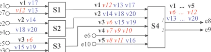
Figure 1 shows an example of a switched Ethernet network

configuration which consists of 4 switches,S1toS4,

intercon-necting 10 end systems,e1 toe10, through full duplex links

to transfer 20 flows,v1 tov20. In this work, each output port

of a switch has a set of buffers controlled by a Deficit Round Robin (DRR) scheduler. The links provide a bandwidth of R = 100 M bits/s. Table I summarizes flow features

(inter-arrival durationTi as well as minimum and maximum frame

sizelmin

i andlmaxi ).

III. DEFICITROUNDROBIN

In this section, we briefly recall the DRR scheduling policy. A more detailed description can be found in [6] and [7]. We

e1 e7 e2 e4 e5 e6 e3 v1 e10 v12 v17 v13 v2v14 v18 v20 v6 v3 v15 v19 v12 v1 v13 v17 v2v14 v18 v20 v6 v3 v15 v19 v7 v9 v10 v4 v8 v11 v5 v16 v1 ... v5 v6 ... v12 v13 ... v20 S4 1 2 e8 e9 S2 S1 S3

Fig. 1: Switched Ethernet network (Example 1) TABLE I: Network Flow Configuration

Flows vi Ti(µsec) lmaxi (byte) lmini (byte)

v12, v20 512 100 80

v1, v7, v8, v9, v17 512 99 80

v2, v4, v5, v10, v13, v16, v18 256 100 80

v3, v11, v14, v15, v19 256 99 80

v6 96 100 80

then summarize the DRR worst-case analysis in [7], [8]. This analysis is based on network calculus [1].

A. DRR scheduler principle

DRR was designed in [6] for a fair sharing of server capacity among flows. DRR is mainly a variation of Weighted Round Robin (WRR) which allows flows with variable packet length to fairly share the link bandwidth.

The flow traffic in a DRR scheduler is divided into buffers based on few predefined classes. Each class receives service sequentially based on the presence of a pending frames in a class buffer and the credit assigned to the class. Each class buffer follows FIFO queuing to manage the flow packets. The DRR scheduler service is divided into rounds. In each round all the active classes are served. A class is said to be active when it has some flow packet in output buffer waiting to be transmitted. The basic idea of DRR is to assign a credit

quantumQh

x to each flow classCx at each switch output port

h. Qh

xis the number of bytes which is allocated toCxfor each

round at porth. At any time, the current credit of a class Cx

at a porth is called its deficit ∆h

x. Each timeCx is selected

by the scheduler, Qh

x is added to its deficit∆hx. As long as

Cx queue is not empty and∆hx is larger than the size ofCx

queue head-of-line packet, this packet is transmitted and∆h

x

is decreased by this packet size. Thus, the scheduler moves

to next class when either Cx queue is empty or the deficit

∆h

xis too small for the transmission ofCxqueue head-of-line

packet. In the former case, ∆h

x is reset to zero. In the latter

one, ∆h

x is kept for the next round.

The credit quantumQh

x is defined for each port h. It must

allow the transmission of any frame from class Cx crossing

h. Thus, Qh

x has to be at least the maximum frame size of

Cx flows at port h. Let FChx be the set of flows of classCx

at output port h. Let lmax,h_Cx andl_Cmin,h_x be the max and min

frame size among all classCxflows at output porth. We have:

lmax,hCx = max i∈Fh Cx lmaxi , l min,h Cx = min i∈Fh Cx limin (1)

Algorithm 1 shows an implementation of DRR at a switch

(lines 1-3). Then queues are selected in a round robin order (lines 4-16). Empty queues are ignored in each round (line 6).

Each non-empty queue is assigned an extra credit of Qh

i in

each round (line 7). Packets are sent as long as the queue is not empty and the deficit is larger than the size of the head-of-line packet (lines 8-12). If the queue becomes empty, the deficit is reset to 0 (lines 13-14).

Let us illustrate DRR with the network configuration in

Figure 1. Three traffic classes are considered. C1 includes

flows v1 to v5 (in black and bold font in Figure 1), while

C2 includes flowsv6 tov12 (in red and italics font in Figure

1) andC3 includes flowsv13 tov20(in blue and regular font

in Figure 1), as listed in Table II.

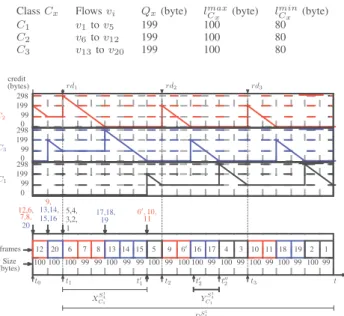
Figure 2 shows a possible scenario for DRR scheduling in

the upper port of switchS4 (port S1

4). All the flows in Figure 1

cross this port. In the example in Figure 2, the credit quantum

QS

1 4

x is 199 bytes (1592 bits) for each classCx (x = 1, 2, 3).

It is larger than the maximum frame size lmax,S

1 4 Cx for each class at port S1 4. Indeed, we have l max,S1 4 Cx = 100 bytes for 1 ≤ x ≤ 3.

TABLE II: DRR scheduler configuration

Class Cx Flows vi Qx(byte) l_Cmax_x (byte) lmin_Cx (byte)

C1 v1to v5 199 100 80 C2 v6to v12 199 100 80 C3 v13to v20 199 100 80 rd1 credit rd2 rd3 C3 C1 298 199 99 0 (bytes) C2 5,4, 20 11 9, 19 12,6,13,14, 7,8, 15,16 3,2, 1 17,18, 6′_{, 10,} Size frames XS1 4 C1 DS1 4 1 t1 t2 t3 10 11 18 19 4 3 2 1 100 99 100 99 100 99 100 99 6′ 9 15 5 16 17 99 100 99 100 100 99 12 20 6 7 8 13 14 100 99 99 100 99 100 100 t t′ 1 t′2 t′′2 t0 (bytes) 298 199 99 0 298 199 99 0 YS1 4 C1

Fig. 2: DRR rounds at output portS1

4

In the scenario in Figure 2, there are no pending frames

before time t0 in output port S41. At this time, five frames

arrive: four belonging to classC2 (from flowsv12,v6,v7 and

v8 in this order in the queue) and one belonging to classC3

(from flowv20). Since there are no pending frames beforet0,

eitherC2orC3can be served first. In Figure 2, we assume that

classC2is served first. Thus, att0,C2 receives a credit equal

to its assigned quantum value, we have∆S

1 4

2 = 199 bytes. The

size ofC2 head-of-line packet is 100 bytes (fromv12). Since

it is smaller thanC2 current deficit,v12 packet is transmitted

andC2 deficit becomes ∆

S1 4

2 = 199 − 100 = 99 bytes. The

newC2 head-of-line packet (fromv6) of 100 bytes is larger

than remaining deficit. Thus, it cannot be transmitted and next

active class (C3) is served. Now C3 gets credit equal to its

assigned quantum value, so we have ∆S

1 4

3 = 199 bytes. C3

head-of-line packet (flow v20) has a size of 100 bytes. Thus,

it is immediately transmitted and∆S

1 4

3 is reduced to 99 bytes.

Meanwhile, five new frames from flowsv9,v13,v14,v15and

v16arrive in portS41and they are buffered in their class queue.

NewC3 head-of-line packet (fromv13) is larger than current

credit and cannot be transmitted leaving a deficit ∆S

1 4

3 = 99

bytes and next active classC2 can be served. Indeed,C1 has

no pending packet at that time. Credit QS

1 4 2 is added to∆ S1 4 2 ,

leading to a deficit of 298 bytes. Three C2 pending packets,

from flowsv6,v7 andv8, have a cumulated size of 298 bytes.

Thus, they are all transmitted in the current round, leading to

a null deficit for C2. The same occurs for next active class

C3, with v13, v14 andv15 packets. Next active class is C1.

Indeed, packets from v5, v4,v3, v2 andv1 have arrived. C1

deficit ∆S

1 4

1 is 199 bytes. It allows the transmission of the

first pending frame (from v5) and ∆S

1 4

1 is 99 bytes. Frame

transmissions go on in the same manner. Algorithm 1: DRR Algorithm

Input: Per flow quantum:Qh

1. . . Qhn (Integer)

Data: Per flow deficit:∆h

1. . . ∆hn(Integer)

Data: Counter: i (Integer)

1 fori = 1 to n do 2 ∆h_i ← 0 ; 3 end 4 whiletrue do 5 fori = 1 to n do 6 ifnotempty(i) then 7 ∆h_i ← ∆h_i + Qh_i;

8 while(notempty(i)) and

(size(head(i)) ≤ ∆h i) do 9 send(head(i)); 10 ∆h_i ← ∆h_i − size(head(i)); 11 removeHead(head(i)); 12 end 13 ifempty(i) then 14 ∆h_i ← 0 15 end 16 end

B. DRR scheduler worst-case analysis

Worst-case traversal time (WCTT) analysis is needed when real-time flows are considered. Indeed, the latency of these flows has to be upper bounded. In this section, we analyze flow latency when a DRR scheduler is used. Then we summarize the state-of-the-art WCTT analysis [7], [8], based on network calculus [1].

1) DRR scheduler latency: A DRR scheduler schedules

nh _{traffic classes at a given output port h. Each class C}

x

is assigned a quantumQh

Definition 1. Theoretical service rate: The quantum Qh x

allocated to traffic classCx at porth defines the theoretical

service rateρh

x ofCx ath, i.e. the minimum service rate that

Cx should get on the long term. We have

ρh x= Qh x P 1≤j≤nh Qh j × R (2)

In the example in Figure 2, output port S1

4 is shared by

nS1

4 = 3 classes (C

1, C2 and C3). All of them are assigned

a quantum of 199 bytes (1592 bits). Thus, the theoretical

service rate for any classCx can be computed by Equation

(2): ρS 1 4 x = 199 199 ∗ 3× 100 M bits/s = 100 3 M bits/s

However the service provided to Cx at h in a given time

interval might be more or less than the theoretical one. Definition 2. Actual service rate: The actual service rate is

the service rate received by a given classCx at a porth in a

given time interval.

The actual service rate of a given class depends on the packets which effectively cross the output port. First, as

previ-ously defined, a class is active in an output porth when it has

pending packets inh. In a given time interval, active classes

share the available bandwidth. For instance, considering port S1

4 in Figure 2,C2 andC3 each get half of the bandwidth in

any interval where they are active andC1 is not. Thus, a class

can receive more than its theoretical service rate when some other classes are inactive. Second, since frames are transmitted sequentially, each class is served on its turn, thus getting 100 % of service for some duration. Third, since a packet cannot be transmitted in the current round if its size is more than the remaining credit of its class, a class might get less than its theoretical service rate in a round. Conversely, since the credit which is not used by a class in a round might be used in the following round, a class can get more than its theoretical service rate in a round.

The aim of a WCTT analysis is to maximize the latency of a given flow. It can be obtained by minimizing the actual service rate of its class. In [8], it is based on the DRR scheduler latency.

Definition 3. DRR scheduler latency: The DRR scheduler

latency Θh

x experienced by a class Cx flow at output port

h is defined as the maximum delay before Cx flow is served

at its theoretical service rateρh x.

[8] determines a lower bound on the service thatCxreceives

in a given interval. To that purpose, it introduces two delays at the beginning of the considered interval:

• the delay X_Ch_x before class Cx receives service for the

first time in the interval,

• a delayY_Ch_x to take into account the fact that, when Cx

receives service for the first time, it can be a reduced service.

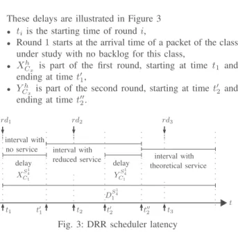
These delays are illustrated in Figure 3

• ti is the starting time of roundi,

• Round1 starts at the arrival time of a packet of the class

under study with no backlog for this class,

• X_Ch

x is part of the first round, starting at time t1 and

ending at timet′

1, • Y_Ch

x is part of the second round, starting at timet

′ 2 and ending at timet′′ 2. XS 1 4 C1 DS 1 4 1 t1 t2 t3 t t′ 1 t′2 t′′2 rd1 rd2 rd3 delay YS 1 4 C1 delay reduced service interval with theoretical service interval with no service interval with

Fig. 3: DRR scheduler latency

Let us come back to the example in Figure 2 in order to

illustrate the first duration (the delayXh

Cx before first service).

The firstC1 packet arrives at timet1, where it just misses its

turn to receive service. Before receiving the first service, it has to wait till timet′

1 while all the other active classes (C2,C3)

are served. This delay has been analyzed and upper bounded

in [8]. It is denoted byXh

x for classCxin nodeh. It has been

shown in [8] that it is maximized when classCxhas to wait for

all the other classes with maximum transmission capacity. This maximum delay can be computed by the following formula:

Xh x = P j={1,2,...,nh_{}, j6=x} (Qh j+ ∆ max,h j ) R (3)

where∆max,hj is the maximum deficit of class Cj in nodeh

at the end of its service. Since classCjpackets are served as

long as the remaining deficit of classCj is not smaller than

the size of classCjhead-of-line packet, the remaining deficit

has to be smaller than the largestCj packet. Thus, we have:

∆max,h x = l

max,h

Cx − 1 (4)

wherelCmax,hx is the size of the largestCx packet.

This maximum delay is observed for class C1 in round

rd1 in Figure 2. Indeed, classesC2 andC3 have a maximum

remaining deficit at timet1:

∆max,h₂ = lmax,hC2 − 1 = 100 − 1 = 99 bytes ∆max,h3 = lmax,hC3 − 1 = 100 − 1 = 99 bytes

Both classes (C2, C3) get maximum service between t1 and

t′

1. They both have a credit of 199 + 99 = 298 bytes. It

corresponds to the cumulative size of pending packets forC2

(v6,v7andv8packets) as well asC3(v13,v14andv15packets).

Thus, the delay until firstC1 pending packet (fromv5) gets

transmitted is computed by Equation (3):

XS 1 4 1 = (298 + 298) ∗ 8 100 = 47.68 µs

The second delay Yh

Cx comes from reduced service. It can

also be illustrated with the example in Figure 2. In rd1, C1

receives a reduced service (100 bytes corresponding to the

transmission of av5packet). Indeed, the remaining deficit (99

bytes) is smaller than head-of-lineC1packet (100 bytes forv4

packet) Thus,C1receives at least its theoretical service rate in

rd2, after the service ofC2andC3 (199 bytes for each class

in Figure 2). It means that, betweent′

1 andt′′2,C1 receives a

service of 100 bytes. Since, betweent′

1 andt′′2, 498 bytes are

transmitted (packets fromv5,v9,v6,v16andv17),C1receives

an average service of 100

498× 100 ≃ 20 M bps

instead of one third of the available bandwidth, i.e. 33.33 Mbps. Another solution to compute the average service for

C1 betweent′1 andt′′2 is to split the interval in two parts:

• in the first part,C1 receives an average service of one

third of the available bandwidth,

• in the second part, it receives no service.

SinceC1 gets a service of 100 bytes att′1, it gets on average

one third of the available bandwidth betweent′

1andt′2. Indeed,

300 bytes are transmitted between these two instants. Then,

C1 gets no service between t′2 and t′′2. These intervals are

illustrated in Figure 3

In [8], the computation of the largest possible duration of such an interval with no service is formalized. The authors in [8] prove an upper bound on this duration and show a scenario leading to this upper bound. We compute the duration corresponding to such a scenario and show that it corresponds

to a worst-case. This worst-case durationYh

x for a class Cx

in a nodeh is given by:

Yh x = Qh x− ∆max,hx + P 1≤j≤nh j6=x Qh j R − Qh x− ∆max,hx ρh x (5)

The first fraction computes the duration between t′

1 and t′′2,

while the second one corresponds to the duration between t′

1 and t′2. The delay t′′2 − t′2 is the impact of the reduced

service on class Cx. The first fraction corresponds to the

situation where classCxreceives its minimum possible credit

Qh

x−∆max,hx (its deficit for the following round is maximized)

while other classes receive exactly the credit corresponding to their quantum. The second fraction computes the duration of

a round where classCx receives its minimum possible credit

and its theoretical service rate.Yh

x can be greater if one class

Cj(j 6= x) receives more than its quantum in round rd2:Cj

receives a credit ofQh

j+d with 0 < d ≤ ∆

max,h

j . In that case,

Cjhas a deficit of at leastd form round rd1. However, in the

computation of Xh

x, we consider that class Cj consumes its

maximum possible creditQh

j+ ∆ max,h

j inrd1, leading to no

deficit. Thus, adding a credit ofd to class Cjinrd2comes to

remove a credit of at leastd from Cjin roundrd1. Therefore

it does not increase the sumXh

x+ Yxh

Considering the example in Figure 2, it gives:

YS 1 4 1 = (199 − 99) ∗ 8 + (199 + 199) ∗ 8 100 − (199 − 99) ∗ 8 100 3 = 15.84µs

This scenario in Figure 2 corresponds to a worst-case for class

C1, with maximum values forX

S1 4 1 andY S1 4 1 .

Finally, the DRR scheduler latency Θh

x is defined as the

delay beforeCxpackets are served at their theoretical service

rate at porth. Thus:

Θh

x= Xxh+ Yxh (6)

In the example in Figure 2, we have:

ΘS 1 4 1 = X S1 4 C1+ Y S1 4 C1 = 63.52 µs

2) Network Calculus applied to DRR scheduling: WCTT analysis for DRR has been modeled with Network Calculus in [7]. In this paragraph, this modeling is summarized. The Network Calculus (NC) theory is based on the (min, +) algebra. It has been proposed for worst-case backlog and delay analysis in networks [1]. It models traffic by arrival curves and network elements by service curves. Upper bounds on buffer size and delays are derived from these curves.

a) Arrival Curve: The traffic of a flowvi at an output

porth is over-estimated by an arrival curve, denoted by αh

i(t).

The leaky bucket is a classical arrival curve for a sporadic traffic:

αh

i(t) = r × t + b, f or t > 0 and 0 otherwise.

It can be used to model a flowviat its source end systemek.

We have: αej i (t) = lmax i Ti × t + lmax i , f or t > 0 and 0 otherwise.

It means that vi is allowed to send at most one frame of

maximum lengthlmax

i bits every minimum inter-frame arrival

timeTi µs.

Any flow vi can be modeled in a similar manner at any

switch output port h it crosses. However, since a frame of

flow vi can be delayed by other frames before it arrives at

port h, a jitter Jh

i has to be introduced. It is the difference

between the worst-case delay and the best-case delay for a

frame of flowvifrom its source end system to porth [2].

Since flows of classCxare buffered in their class queue and

scheduled by FIFO policy, an overall arrival curve is used to

constrain the arrival traffic of classCxat porth. It is denoted

byαh

Cx and calculated by:

αh Cx(t) = X i∈Fh Cx αh i(t) (7) whereFh

Cx is the set ofCx flows crossing porth.

As an example, let us consider the output port S1

4 in

toFS 1 4

C1 = v1, v2, v3, v4, v5. The overall arrival curve of class

C1 can be computed by:

αS 1 4 C1(t) = X i∈FS 1 4 C1 αS 1 4 i (t)

which is illustrated by blue line in Figure 4a.

bits QS 1 4 1-∆ max,S1 4 1 DS 1 4 1 1 R 1 t (µsec) sl αS1 4 C1 P i∈FS 1 4 C1 (bi) XS1 4 C1Y S1 4 C1 ΘS1 4 C1 βS 1 4 C1 ρS 1 4 C1 P 1≤j≤3 QS1 4 j−∆ max,S1 4 1 R bits Qh x-∆max,hx Dh i 1 R 1 t (µsec) sl αh x,SER P i∈Fh Cx (bi) Xh x Yxh Θh x βh x ρh x max i∈Fh x (bi)

(a) NC curves at S41 (b) NC Curves with serialization

Fig. 4: NC curves atS1

4

b) Service Curve: According to NC, the full service

provided at a switch output port h with a transmission rate

ofR (bits/s) is defined by:

βh_{(t) = R[t − sl]}+

wheresl is the switching latency of the switch, and [a]+_means

max{a, 0}.

According to [8] and [7], the full service is shared by

all DRR classes at an output port h and each class Cx has

a predefined service rate ρh

x based on its assigned credit

quantum Qx as explained in Section III-B Equation (2).

Besides a reduced service rate, each classCxcould experience

a DRR scheduler latencyΘh

xbefore receiving service with the

predefined rate ρh

x. The scheduler latency can be calculated

by Equation (6). Therefore, based on the NC approach, the

residual serviceβDRR

Cx to each classCxis given by:

βh

Cx(t) = ρ

h

x[t − Θhx− sl]+ (8)

Yh

x delay is considered right afterXxh, in order to get a convex

service curve.

In the example of the output portS1

4, classC1service curve

is: βS 1 4 C1(t) = ρ S1 4 1 ∗ [t − Θ S1 4 1 − sl]+= 100 3 (t − 63.52 − sl) +

which is illustrated in Figure 4a.

The actual service curve is a staircase one (shown by the dashed black line in Figure 4a), as a flow alternates between being served and waiting for its DRR opportunity, as explained in [8]. For computation reason, NC approach employs the convex curve represented by equation (8) which is an under-estimated approximation of actual staircase curve.

c) Delay bound:According to NC, the delay experienced

by aCx flowvi constrained by the arrival curveαhCx(t) in a

switch output porth offering a strict DRR service curve βh

Cx(t) is bounded by the maximum horizontal difference between the

curvesαh

Cx(t) and β

h

Cx(t). Let D

h

i be this delay. It is computed

by: Dh i = sup s≥0(inf{τ ≥ 0|α h Cx(s) ≤ β h Cx(s + τ )}) (9)

Therefore, the end-to-end delay upper bound of aCx flow

viis denoted byDET Ei and it is calculated by:

DET E i = X h∈Pi Dh i (10)

Based on the equation (9) and (10), the delay bound

calcu-lated for flowv1of classC1 is found to beDS

1 4

1 = 234.91 µs

andDET E

1 = 387.63 µs.

IV. PESSIMISM OFDRR WCTTANALYSIS

The delay upper bound Dh

i for flow vi from class Cx

presented in the previous section assumes that, at each output

porth, every interfering class Cyconsumes maximum service.

More precisely, it assumes that, in any DRR roundrdk, each

classCy (y 6= x) is always active and transmits frames of at

least the size of its quantum value Qh

y. Such an assumption

might be pessimistic. Indeed, the traffic from one or several

Cyclasses might be too low to consume quantum valuesQhy

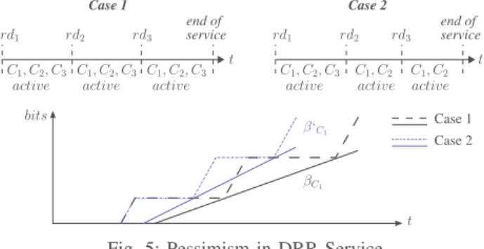
in each round. The effect of such a pessimism on service curve is shown in Figure 5. bits t rd1 rd2 rd3 C1, C2, C3 active C1, C2 active t rd1 rd2 rd3 service C1, C2, C3 active C1, C2, C3 active t C1, C2, C3 active C1, C2 active Case 1 Case 1 Case 2 Case 2 β‘C1 βC1 end of service end of

Fig. 5: Pessimism in DRR Service

This pessimism can be illustrated with the example in Figure 6. This example is based on the network architecture in Figure

1. The difference is that part of C2 and C3 flows that are

transmitted fromS4toe8 in Figure 1 are transmitted toe9 in

Figure 6. S2 S1 S3 e6 v12 v1 e172e14 v2e152e162e30 v6 v3 e1v2e18 v7 v9 v10 v4 v8 v11 v5 e1 e10 S41 2 v1 ... v5 v6 v7 v8 v12 e172e152e1v2e30 v9 ... v11 e1 2299922e18 . 6 . 8

Fig. 6: Switched Ethernet network (Example 2)

We focus on output portS1

4 to calculate the delay

worth noting that the considered classC1has more flows to be

served as compared to the classC2andC3. The corresponding

DRR schedule rounds are shown in Figure 7. The scenario in

rd1 credit rd2 rd3 C3 C1 298 199 99 0 (bytes) C2 5,4, 3,2, 1 6′ Size frames XS 1 4 C1 DS41 1 t1 t2 t3 4 3 2 1 100 99 100 99 6′ 15 5 99 100 7 8 6 13 14 100 99 99 100 99 100 t 20 12,6, 14,15 7,8, 13, 12 100 20 100 t0 t′1 t′2 (bytes) 298 199 99 0 298 199 99 0 Fig. 7: DRR cycles atS1 4

the example given in Figure 7 is similar to the scenario in

Figure 2, where the firstC1 packet arrive at time t1 and it

experience a delayXS

1 4

C1 = 47.68 µs before being served for

the first time. As shown in Figure 7, att′

1, classC3has served

all its frames in the buffer, by transmitting frames fromv13,

v14 and v15. Its deficit is reduced to∆S

1 4

3 = 0 and it has no

more frames to further delay classC1 flows. Similarly, class

C2consumes all its deficit by transmitting frames fromv6,v7

and v8 and its deficit is also reduced to ∆S

1 4

2 = 0. Another

frame from flowv6 has arrived att′1. Att2, classC2 receive

service of100 bytes (corresponding to frame of v6). At t′2,

there are no more frames from classC2 andC3to be served,

classC1 gets the deficit of∆S

1 4

1 = 199 + 99 = 298 bytes to

serve frames from v4 and v3. Since the remaining deficit is

less than the size of next frame fromv2, and there are no other

active classes, classC1 receives an additional credit equal to

its quantum value. Thus, it has a deficit of∆S

1 4

1 = 298 bytes

to serve v2 and v1 flows. Betweent1′ and t′2, C1 receives a

service of 100 bytes. Since, betweent′

1 andt′2, 200 bytes are

transmitted, it meansC1 received an average service of

100

200× 100 = 50 M bps

which is greater than its theoretical service rate (from equation

(2)) ρS

1 4

1 = 199+199+199199 × 100 = 33.33 M bps Thus, in

this scenario class C1 flows do not experience any reduced

service. Therefore, the total latency observed by classC1flows

before they could be served at their theoretical service rate is 47.68 µs, which is much less than that considered by the NC

approach i.e. 47.68 + 15.84 = 63.52 µs. In this case, the

delay bounds, calculated from Equation (9) and (10), for flow

v1 of classC1areDS

1 4

1 = 215.9 µs and DET E1 = 366.87 µs.

However, the scenario in Figure 7 might not lead to the worst-case. In next section, we show how to upper bound the effective impact of interfering classes.

V. TAKING INTO ACCOUNT THE EFFECTIVE LOAD OF INTERFERING CLASSES

As illustrated in the previous section, maximizing the ser-vice of interfering classes when computing the worst-case

end-to-end delay for packets of a given class Cx can introduce

pessimism, since these interfering classes might generate too few traffic to consume all their allocated service. In this section we show how it is possible to upper bound the traffic of these interfering classes that impact the worst-case delay of

Cx packets. Each time this upper bound is smaller than the

maximized service for interfering classes, the difference can

be safely removed from the worst-case delay ofCx packets.

The approach considers the following steps.

1) We compute the worst-case delayDh

x of classCxflows

in nodeh, using the NC approach from [8], [7] presented

in previous sections (equation (9) and (10)). Indeed, all the flows of a given class experience same delay at a given output port.

2) We determine the service loadSLh

y(t) available for class

Cyat a nodeh between 0 and Dxh. It corresponds to the

maximized service of interfering classesCyused by the

NC approach from [8], [7].

3) We calculate the effective maximum loadLmax,h

y (t) of

a class Cyat a node h between 0 and Dhx. It gives an

upper bound on theCytraffic which has to be served at

nodeh between 0 and Dh

x.

4) If Lmax,h

y (Dhx) < SLhy(Dhx), the difference can be

safely removed from the worst-case delayDh

x of class

Cx flows in nodeh

The first step is a direct application of what has been presented in previous sections. The three other steps are detailed in the following paragraphs.

A. Maximized service of interfering classes

The NC approach in [8], [7] considers a maximized service

for an interfering classCythat is not the same for all the time

intervals. The time starts when the firstCx frame arrives at

nodeh.

• The first interval (0,X_xh] corresponds to the delay Xh

x

beforeCxis served for the first time. In this interval, the

NC approach assumes thatCy gets a service of at most

Qh

y+ ∆max,hy bytes.

• The second interval starts atXh

x and stops whenCxgets

service for the second time. In this interval, Cx gets a

service ofQh

x− ∆max,hx bytes while each other classCy

gets a service of Qh

ybytes.

• The following intervals are all identical. As in the second

one, each Cy class gets a service of Qhy bytes. The

difference with the second interval is that Cx class also

gets a service ofQh

x bytes. Thus, each of these intervals

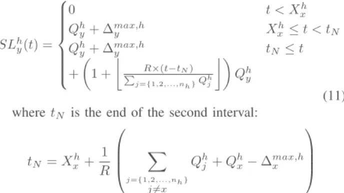
Thus, the maximized service loadSLh y(t) is defined as fol-lows: SLh y(t) =              0 t < Xh x Qh y+ ∆max,hy Xxh≤ t < tN Qh y+ ∆max,hy tN≤ t + % 1 + & R×(t−tN) P j={1,2,...,nh}Qhj '( Qh y (11)

wheretN is the end of the second interval:

tN= Xxh+ 1 R     X j=_{1,2,...,nh} j6=x Qh j + Qhx− ∆max,hx    

It should be noticed that the load corresponding to a given interval is taken into account at the end of the interval. For

instance,Qh

y+ ∆max,hy is added toSLhy(t) at the end of the

first interval, i.e.t = Xh

x. Thus,SLhy(t) is an under-bound

of the maximized service load considered in [8]. We obtain a step function, as illustrated in Figure 8.

XS 1 4 1 t tN _t N+ 3 P j=1Q S1 4 j R 0 Served QS1 4 2 + ∆ max,S1 4 2 2QS1 4 2 + ∆ max,S1 4 2 3QS1 4 2 + ∆ max,S1 4 2 traf f ic 3 P j=1 QS 1 4 j R 696 bytes 497 bytes 298 bytes

Fig. 8: Served traffic of classC2

Considering the example in Figure 6, for any value t, we

have: SLS 1 4 C2(t) =            0 t < 47.68 298 bytes 47.68 ≤ t < 87.52 298+ 87.52 ≤ t / 1 +0 100 8 ×(t−87.52) 597 12 199 bytes

By applying the NC computation, we obtainDS

1 4

1 = 223.32µs.

Thus, the maximized load of an interfering class Cy in the

service durationt = DS

1 4

1 of classC1 flowv1 is:

(SLS 1 4 C2(D S1 4 1 )) = (SL S1 4 C3(D S1 4 1 )) = 895 bytes

B. Effective maximum load of interfering classes

The effective maximum load Lmax,h

y (t) of an interfering

class Cy at a node h in a given duration t is based on the

arrival curves of NC. Thus,Cy load at the beginning of the

duration is the sum of all the bursts ofCyflow arrival curves

and it increases, following the long-term rate of eachCyflow

arrival curve. Since the delay of classCx flows in nodeh is

upper bounded byDh

x, only packets arriving within a duration

Dh

x have a chance to delay a givenCxpacket. Thus,Cy load

that can delay a givenCxpacket is upper bounded by:

Lmax,hy (D h x) = α h Cy(D h x) (12) whereαh

Cy(t) is the overall arrival curve of the class Cyflows,

calculated by Equation (7).

Considering the example in Figure 6, we have DS4

1 =

223.32 µs, as depicted in the upper part in Figure 9a. The

lower part in Figure 9a shows the overall arrival curve ofC2

flows inS4. Thus, we have:

Lmax,S 1 4 C2 (D S4 1 ) = 858 bytes

Similarly, forC3 flows, we have:

Lmax,S 1 4 C3 (D S4 1 ) = 784 bytes bits DS14 1=223.32 t (µsec) αS41 C2 P i∈FS14 C2 (bi) Lmax,S14 C2 sl+ ΘS14 C1 1 ρS41 C1 bits αS41 C1 P i∈FS14 C1 (bi) t=223.32 t (µsec) βS41 C1

(a) Arrival traffic of C2

bits t _t (µsec) αh Cy P i∈Fh Cy (bi) Lmax,h_C y bits t (µsec) P i∈Fh Cx (bi) max i∈Fh Cx (bi) Dh x αh SERCx ρh Cx 1 max i∈Fh Cy (bi) sl+ Θh Cx βh Cx

(b) Arrival traffic of Cy with

grouping

Fig. 9: Arrival traffic

C. Limitation of the service to the load

In previous paragraphs, we have computed for each class

Cy interfering at nodeh with class Cx under study:

• the service load SLh

y(t) taken into account by the NC

approach in [8], [7],

• an upper boundLmax,h

y (t) on the effective load.

When this upper bound is smaller than the service load taken into account by the NC approach, the difference can be safely

removed from the delay of Cx flow vi packets in node h.

Indeed, in a round, when a class Cy has nothing more to

transmit, DRR moves to the next class, which is then served

earlier. Therefore, followingCxpackets will be served earlier,

leading to a reduced delay.

Thus, for each interfering class Cy we can remove the

following value:

max3SLh

y(Dxh) − Lmax,hy (Dhx), 0

4

Sincenh− 1 classes are interfering with Cx in node h, the

optimized delayDh

i,opt forCx flowviin nodeh is given by:

Dh i,opt= Dhi − P y∈1...nh y6=x max3SLh y(Dxh) − Lmax,hy (Dhx), 0 4 R (14)

Therefore, the end-to-end delay upper bound of a class Cx

flowvi can be computed by:

DET E i,opt = X h∈Pi Dh i,opt (15)

In the example in Figure 6,DS

1 4

1,opt is211.59µs and DET E1,opt

is300.86µs, which gives 19.8% improvement in ETE delay

computation as compared to theDET E

1 = 375.34µs.

VI. FURTHER IMPROVEMENTS

In this section, we present three further improvements of the worst-case delay computation. The first one concerns the

additional delay Yh

x generated by the reduced service for

classCx when it is first served. The second one is based on

the integration of the serialization effect: packets sharing an input link cannot arrive in the output node of the link at the same time. The third one concerns flow scheduling at end systems: integration of offset. The effect of integrating these improvements in NC approach is evaluated on an industrial configuration and shown in Table IV.

A. Optimization ofYh x latency

The duration Yh

x of class Cx at an output port h is

computed by considering that, whenCxis served for the first

time, it consumes exactly its minimum possible service, i.e.

Qh

x− ∆max,hx , where ∆max,hx is the size of the largest Cx

packet crossing porth minus one byte. If we assume a port h

where allCxpackets have a size of 100 bytes and the quantum

Qh x is 150 bytes, we have: ∆max,hx = 100 − 1 = 99 bytes Thus, Qhx− ∆ max,h x = 150 − 99 = 51 bytes

In that case, the computation ofYh

x considers thatCxtransmits

51 bytes when it is served for the first time.

However, since DRR imposes that Qh

x is at least the size

of the largestCx frame (here150 ≥ 100), one Cx packet is

guaranteed to be transmitted when Cx is served for the first

time. In our case, 100 bytes will be transmitted during the first

Cx service. Thus, considering only 51 bytes significantly

un-derestimate this first service and it leads to an overestimation

ofYh

x.

In the general case, at least one Cx packet with minimum

size is transmitted. Thus, the minimum first service for Cx

cannot be less than this minimum sizelmin,h_Cx . DRR guarantees

that it cannot be less thanQh

x− ∆max,hx . Therefore it cannot

be less than

max{Qh

x− ∆max,hx , l min,h Cx }

This upgraded minimum first service for Cx can be

inte-grated in the computation ofYh

x. We get: Yh x = max₍Qh x−∆ max,h x ,l min,h Cx )+ P 1≤j≤nh j$=x Qh j R − max₍Qh x−∆max,hx ,lmin,hCx ) ρh x (16)

B. Integration of DRR/FIFO Serialization

As explained in Section III-B2a, the arrival curve for a class

Cx in a porth is obtained by summing the arrival curves of

allCxflows inh. This operation assumes that one frame from

each flow arrives exactly at the same time inh. This situation

might be impossible. Let us come back to the example in

Figure 1.C3flowsv14,v18andv20share the link betweenS2

andS4. Therefore they cannot arrive inS4 at the same time.

They are serialized on the link.

This serialization effect has been integrated in the NC approach for FIFO [2]. The idea is to consider that the largest packet among the flows sharing the link arrives first. Packets from the other flows arrives by decreasing size, at the speed of the link.

This approach can be adapted to DRR scheduling. Indeed, DRR scheduling considers each class separately. Therefore, the serialization effect can be integrated as in [2], on a class by class basis. The principle of a curve integrating serialization is illustrated in Figure 4b.

These serialized arrival curves are then directly used for the worst-case delay computation.

While considering serialization with our optimized NC approach, one should pay attention while calculating effective maximum load of interfering classes (section V-B). In this case

one should use the arrival curve and time valuet (≥ Dh

x) as

shown in Figure 9b.

C. Flow scheduling at end system

In a switched Ethernet network each end system schedules flow transmission individually. The flow scheduling introduces temporal separation between flows and hence reduce the effec-tive traffic in the network. The scheduling of flows emitted by given end system is characterized by the assignment of offsets which constrain the arrival of flows at output ports. The offset integration in NC was first proposed in [14] for First-In-First-Out (FIFO) scheduler. A Similar approach can be used for DRR schedulers.

The idea is that, if the flows are temporally separated at source end system and they share the same input link then they cannot arrive at an output port at the same time. Such flows can be aggregated as a single flow.

[14] defines relative offsetOh

r,b,i at an output porth as the

minimum time interval between arrival time of a frame from

a reference flowvband arrival time of a frame from another

flowviaftervb. Such offset computation algorithm is given in

[14], however, the aggregation technique can work with any offset assignment algorithm.

In NC, the integration of offset affects the computation of

same source end system, can be aggregated as a single flow.

This is valid because the flows of a classCxtransmitted from

same source end system are affected by temporal separation

and cannot delay each other. ClassCxflows can be aggregated

by taking into account the relative offset at the given node. At

an output porth, for n flows from class Cx the overall arrival

curve αh

Cx, can be computed as :

• Make i subsets of class Cx flows, based on the flows

sharing same source end system. Each subset SSj has

nj flows such thatn1+ n2+ · · · + ni= n.

• Aggregate the flows of each subsetSSias one flow and

characterize its arrival curveαh

SSi. αh SSi= max{α h v1{v2,v3,...vi}, . . . , α h vi{v1,v2,...vi−1}} where,αh

m{n}is the arrival curve obtained when flowvm

arrives before flow vn at output port h, with temporal

separation ofOh

r,m,n.

• The overall arrival curve is the sum of the arrival curve

of each subset, i.e.αh

Cx= i P j=1 αh SSj.

Let us come back to the example in Figure 1, whereC3 flows

v13 . . .v20 compete at output port S41, n = 8, from 6 end

systemse1,e7,e2,e4,e3 ande10. Thus, there are 6 subsets:

SS1 = [v17] (n1 = 1), SS2 = [v13] (n2 = 1) , SS3 = [v14]

(n3 = 1), SS4 = [v18, v20] (n4 = 2), SS5 = [v15, v19] (n5=

2) and SS6= [v16] (n6= 1). The flows v18 andv20 will be

aggregated as one flow to make aggregated arrival curve as

they share source end system e4. Similarly,v15 andv19 will

also be aggregated as one flow. The arrival curve for subsets with only single flow is same as the arrival curve of the flow. For details about the aggregated curve computation, readers can refer to [14].

The obtained overall arrival curve can be used to compute delay using equation (9). It can also be used to calculate

effective maximum load Lh

Cy(t) of interfering class Cy to

optimize the delay using equation (14).

VII. EVALUATION

In this section, we compare the approach in [8] (classical NC DRR) with our optimized approach (optimized NC DRR).

A. Illustrative Example

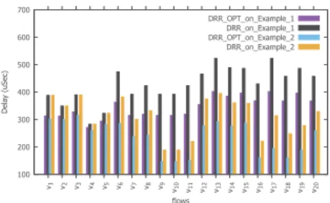
First we consider the sample examples in Figures 1 and 6. Figure 10 shows end-to-end delay bounds obtained by both approaches for each VL of the configuration in Figures 1 and

6. For example in Figure 1, we have average gain13.45%, and

maximum gain19.75%. For Figure 6, average gain is 16.84%

and maximum29.67%.

B. Realistic case study

Next, we consider an industrial-size configuration, inspired from [2]. It includes 96 end systems, 8 switches, 984 flows, and 6412 paths (due to VL multi-cast characteristics).

We take into account three types of flows, namely critical flows, multimedia flows and best-effort data flows. Each flow

100 200 300 400 500 600 700 v1 _v2 _v3 _v4 _v5 _v6 _v7 _v8 _v9 v10 v11 v12 v13 v14 v15 v16 v17 v18 v19 v20 Delay (uSec) flows DRR_OPT_on_Example_1 DRR_on_Example_1 DRR_OPT_on_Example_2 DRR_on_Example_2

Fig. 10: End-to-end delay bound in network example 1 & 2 TABLE III: DRR Scheduler Configuration for Industrial Net-work Class Number of Flows Max Frame Length (byte) Qx (byte) T (msec) Category C1 128 150 3070 4 - 128 Critical C2 590 500 1535 2 - 128 Multimedia C3 266 1535 1535 2 - 128 Best-effort

type is assigned to one DRR class. Table III shows the DRR scheduler configuration.

The results of the optimized NC DRR approach are com-pared with the delays obtained by the classical NC DRR

approach of [7] & [8]. For each pathPx of each flowvi, the

upper bound DPx

i,N C computed by the classical NC approach

is taken as the reference value and it is normalized to 100.

Then the upper bound DPx

i,opt of optimized NC approach is

normalized as DPx i,opt,norm= DPx i,opt DPx i,N C × 100

For illustration purpose, the paths are sorted in increasing order

of DPx

i,opt,norm.

C. Comparison of classical NC with DRR and Optimized NC with DRR

Table V shows the delay computation improvement on applying proposed optimization technique for NC with DRR. As shown in Table V and Figure 11a, 11b, 11c & 11d, the average improvement of the E2E delay bound computed in the given industrial configuration is around 47%. This is a significant improvement which shows that the proposed optimizations are relevant on an industrial configuration. It means that, on such configurations, the load in switch output ports is not equally shared between classes.

D. Comparison of Optimized NC with DRR and Classical NC with FIFO

In Figure 11e and 11f we have compared the delays (com-puted by optimized NC approach) of the different flow classes when using DRR with the delays computed when using FIFO. It can be observed that the critical flows have smaller delays (shown in Figure 11e) than the two other flow classes (shown in Figure 11f) This is due to the fact that, as shown in Table III, DRR approach allows critical flows to have more allocated quanta in each round and hence produces smaller delay.

TABLE IV: Comparison result of improvements applied to classical NC approach

N CSER N COF F N CSER,OF F

NC 5.04 26.98 28.83 Avg Gain %

19.57 70.05 70.05 Max Gain %

TABLE V: Comparison result of optimization applied to different NC approaches

N Cx N C

OP T x

avg gain % max gain %

Classic 47.77 77.55 Offset 48.66 75.38 Grouping 47.2 75.11 Offset + Grouping 48.19 76.59 0 20 40 60 80 100 0 1000 2000 3000 4000 5000 6000 7000 flow paths DRR normalized to 100 DRR_OPT compared to DRR

(a) Classical NC DRR vs. Opti-mized NC DRR 0 20 40 60 80 100 0 1000 2000 3000 4000 5000 6000 7000 flow paths DRR_OFF normalized to 100 DRR_OFF_OPT compared to DRR_OFF

(b) NC DRR with Offset vs. Op-timized NC DRR with Offset

0 20 40 60 80 100 0 1000 2000 3000 4000 5000 6000 7000 flow paths DRR_SER normalized to 100 DRR_SER_OPT compared to DRR_SER

(c) NC DRR with grouping vs Optimized NC DRR with group-ing 0 20 40 60 80 100 0 1000 2000 3000 4000 5000 6000 7000 flow paths DRR_OFF_SER normalized to 100 DRR_OFF_SER_OPT compared to DRR_OFF_SER

(d) NC DRR with Offset & group-ing vs. Optimized NC DRR with offset & grouping

0 20 40 60 80 100 120 140 160 180 200 0 100 200 300 400 500 600 700 800 900 flow paths FIFO_SER normalized to 100 DRR_OPT Compared to FIFO_SER

(e) Optimized NC DRR (Critical flows C1) vs. FIFO 50 100 150 200 250 300 350 0 1000 2000 3000 4000 5000 6000 flow paths FIFO_SER normalized to 100 DRR_OPT Compared to FIFO_SER

(f) Optimized NC DRR (Multime-dia C2 and best-effort C3 flows)

vs. FIFO

Fig. 11: Evaluation of Optimized NC approach

E. Comparison of Optimized NC with DRR and optimized NC with WRR

In this section, we compare our optimized WCTT analysis for DRR with the WCTT analysis for WRR presented in [5]. The WRR analysis cannot cope with the realistic case study presented in previous sections. Indeed, this analysis considers the largest frame size in each class. Since each class includes frames with very different sizes, the computation is very pessimistic and does not converge. This problem is not fully linked to the analysis. It mainly comes from the fact that

WRR cannot cope efficiently with packets with very different sizes in a given class.

A different case study is considered in [5]. It has a similar network architecture as well as a similar number of flows. However, as shown in Table VI, frame sizes are homogeneous per class. Table VII shows that DRR leads to better results

for Classes C1 and C2 and not for C3. Therefore, in that

homogeneous case, no algorithm outperforms the other one. TABLE VI: Configuration of WRR and DRR schedulers

class No. of DRR WRR weight frame size

flows Quantum (bytes) (no. of packets) range

C1 718 4 x lmax 4 415-475

C2 194 2 x lmax 2 911-971

C3 72 1 x lmax 1 1475-1535

TABLE VII: Performance comparison of DRR and WRR schedulers

class DRR vs WRR

avg difference (%) max difference (%)

C1 29.16 52.7

C2 29.6 52.3

C3 -35.4 -68.8

VIII. CONCLUSION

Deficit Round Robin (DRR) scheduling policy has been defined for a fair sharing of server capacity among flows. Bandwidth sharing between traffic classes is fixed by the definition of quantum. DRR is envisioned for future avionics switched Ethernet networks, in order to improve bandwidth usage. It has good fairness properties and acceptable imple-mentation complexity but a non-negligible latency which must be accurately evaluated.

This paper presents an improved method for the WCTT of DRR policy using network calculus. Our approach minimizes the pessimism in delay calculation using network calculus and gives tighter upper bounds on end-to-end delay as compared to previous studies. On an industrial-size case study, the proposed approach outperforms existing ones by 47 %. This improve-ment should allow to increase the number of flows transmitted on the network or to reduce the number of switches. We also show that, thanks to quantum, it is possible to achieve better performance for critical flows as compare to other scheduling policies like FIFO.

The WCTT analysis proposed in this paper is mandatory when critical flows are transmitted on the network. However, one goal of using DRR for avionics network is to be able to share the network between critical flows and less/not critical ones. For those later flows, an upper bound on the delay is not the most relevant metric. Thus, the WCTT analysis has to be coupled with a study of the delay distribution. Such a distribution can be obtained by simulation.

Allocating flows to traffic classes and assigning a quantum to each class has a significant impact on the end-to-end delays. We plan to precisely measure this impact in order to propose guidelines for the tuning of classes and quantum, based on traffic profiles.

REFERENCES

[1] J.-Y. L. Boudec and P. Thiran, Network Calculus: a theory of

determin-istic queuing systems for the internet. LNCS, April 2012, vol. 2050. [2] H. Bauer, J.-L. Scharbarg, and C. Fraboul, “Improving the

worst-case delay analysis of an afdx network using an optimized trajectory approach,” IEEE Trans. Industrial Informatics, vol. 6, no. 4, Nov 2010. [3] H. Charara, J.-L. Scharbarg, C. Fraboul, and J. Ermont, “Methods for bounding end-to-end delays on an afdx network,” Real-Time Systems.

18th Euromicro Conference on. IEEE, p. 10, July 2006.

[4] “Aircraft data network, parts 1,2,7 aeronotical radio inc.” ARINC Specification 664, Tech. Rep., 2002 - 2005.

[5] A. Soni, X. Li, J.-L. Scharbarg, and C. Fraboul, “Wctt analysis of avion-ics switched ethernet network with wrr scheduling,” 26th International

Conference on Real-Time Networks and Systems (RTNS), 2018. [6] M. Shreedhar and G. Varghese, “Efficient fair queuing using deficit

round-robin,” IEEE/ACM Transactions on networking, 1996, vol. 4, no

3, p. 375-385, p. 11, 1996.

[7] M. Boyer, G. Stea, and W. M. Sofack, “Deficit round robin with network calculus,” Performance Evaluation Methodologies and Tools

(VALUETOOLS), 2012 6th International Conference on (pp. 138-147). IEEE, p. 10, October 2012.

[8] S. S. Kanhere and H. Sethu, “On the latency bound of deficit round robin,” Computer Communications and Networks, 2002. Proceedings.

Eleventh International Conference on. IEEE, 2002. p. 548-553., p. 7, October 2002.

[9] M. Boyer, N. Navet, M. Fumey, J. Miggie, and L. Havet, “Combining static priority and weighted round-robin like packet scheduling in afdx for incremental certification and mixed-criticality support,” 5TH

EURO-PEAN CONFERENCE FOR AERONAUTICS AND SPACE SCIENCES (EUCASS), 2013.

[10] L. Lenzini, E. Mingozzi, and G. Stea, “Aliquem: a novel drr implemen-tation to achieve better latency and fairness at o(1) complexity,” IEEE

2002 Tenth IEEE International Workshop on Quality of Service, 2002. [11] Y. Hua and X. Liu, “Scheduling design and analysis for end-to-end

heterogeneous flows in an avionics network,” 2011 Proceedings IEEE

INFOCOM, April 2011.

[12] A. Kos and S. Tomazic, “A more precise latency bound of deficit round-robin scheduler,” Elektrotehnivski vestnik, vol. 76, pp. 257–262, January 2009.

[13] A. Soni, X. Li, J.-L. Scharbarg, and C. Fraboul, “Integrating offset in worst case delay analysis of switched ethernet network with deficit round robbin,” IEEE 23rd International Conference on Emerging Technologies

and Factory Automation (ETFA), 2018.

[14] X. Li, J.-L. Scharbarg, and C. Fraboul, “Improving end-to-end delay upper bounds on an afdx network by integrating offsets in worst-case analysis,” IEEE 15th Conference on Emerging Technologies Factory