Array analysis of the seismic wavefield of long-period events and volcanic tremor at Arenal volcano, Costa Rica

HAL Id: hal-01415993

https://hal.archives-ouvertes.fr/hal-01415993

Submitted on 13 Dec 2016

HAL is a multi-disciplinary open access

archive for the deposit and dissemination of

sci-entific research documents, whether they are

pub-lished or not. The documents may come from

teaching and research institutions in France or

abroad, or from public or private research centers.

L’archive ouverte pluridisciplinaire HAL, est

destinée au dépôt et à la diffusion de documents

scientifiques de niveau recherche, publiés ou non,

émanant des établissements d’enseignement et de

recherche français ou étrangers, des laboratoires

publics ou privés.

Rica

Javier Almendros, Rafael Abella, Mauricio M. Mora, Philippe Lesage

To cite this version:

Javier Almendros, Rafael Abella, Mauricio M. Mora, Philippe Lesage. Array analysis of the seismic

wavefield of long-period events and volcanic tremor at Arenal volcano, Costa Rica. Journal of

Geo-physical Research, American GeoGeo-physical Union, 2014, 119, pp.5536-5559. �10.1002/2013JB010628�.

�hal-01415993�

RESEARCH ARTICLE

10.1002/2013JB010628

Key Points:

• Use seismic array data to analyze LPs and tremor at Arenal volcano in 2004 • Discuss the intriguing differences

between the wavefield of LPs and tremor

• Propose a model to explain them in terms of source position and extent

Correspondence to:

J. Almendros, alm@iag.ugr.es

Citation:

Almendros, J., R. Abella, M. M. Mora, and P. Lesage (2014), Array analysis of the seismic wavefield of long-period events and volcanic tremor at Are-nal volcano, Costa Rica, J. Geophys.

Res. Solid Earth, 119, 5536–5559,

doi:10.1002/2013JB010628.

Received 27 AUG 2013 Accepted 30 MAY 2014

Accepted article online 6 JUN 2014 Published online 2 JUL 2014

Array analysis of the seismic wavefield of long-period events

and volcanic tremor at Arenal volcano, Costa Rica

Javier Almendros1,2_{, Rafael Abella}3_{, Mauricio M. Mora}4,5_{, and Philippe Lesage}6

1_{Instituto Andaluz de Geofísica, Universidad de Granada, Granada, Spain,}2_{Departamento de Física Teórica y del Cosmos,}

Universidad de Granada, Granada, Spain,3_{Observatorio Geofísico Central, Instituto Geográfico Nacional, Madrid, Spain,} 4_{Escuela Centroamericana de Geología, Universidad de Costa Rica, San José, Costa Rica,}5_{Red Sismológica Nacional}

(RSN: UCR-ICE), San José, Costa Rica,6_{ISTerre, Université de Savoie, CNRS, Le Bourget-du-Lac, France}

Abstract

We use wavefield decomposition methods (time domain cross correlation and frequency domain multiple-signal classification) to analyze seismic data recorded by a dense, small-aperture array located 2 km West of Arenal volcano, Costa Rica, and operated during 2.5 days. The recorded wavefield is dominated by harmonic tremor and includes also spasmodic tremor and long-period (LP) events. We find that the initial stages of LP events are characterized by three different wave arrivals. These arrivals propagate with similar back azimuths pointing to the volcano summit (∼80◦N) and increasing apparent slowness of 0.4, 1.1, and 1.7 s/km. Spasmodic tremors cannot be regarded as coherent signals. On the contrary, harmonic tremors are highly coherent, characterized by the stability of the apparent slowness vector estimates. Apparent slowness lays in the range 1–2 s/km. Back azimuths point in the general direction of the volcano but with a large variability (40–120◦N). Nevertheless, there are long-term variations and evidences of multiple simultaneous components in the harmonic tremor wavefield. These observations suggest that LP events and tremor are generated in a shallow source area near the volcano summit, although they do not share exactly the same source region or source processes. The tremor source is located in the shallowest part of the plumbing system, beneath the lava crust. This dynamic region is subject to complex fluctuations of the physical conditions. Degassing events at different locations of this region might generate variable seismic radiation patterns. The effects of topography and heterogeneous shallow structure of the volcano may amplify these variations and produce the wide directional span observed for volcanic tremor. On the other hand, the LP source seems to be more repeatable. LP events are likely triggered by fragmentation of the fluid flow in a slightly deeper portion of the volcanic conduits.

1. Introduction

Arenal volcano is a small stratovolcano (1750 m above sea level (asl)) located in northwestern Costa Rica (Figure 1). It remained eruptive for 42 years, from 1968, when a magmatic andesitic eruption took place after centuries of dormancy [Alvarado et al., 2006], until 2010, when lava effusion gradually stopped. This long-lasting eruption went through different stages set by changes on explosive and effusive activity. The eruption of 29 July 1968 opened three new craters named A, B, and C, from lower to upper [Melson and

Saenz, 1968; Minakami et al., 1969]. During the next few years, basaltic-andesitic lavas were effused from

crater A located at 1050 m asl [Wadge et al., 2006]. In 1974, the activity shifted to crater C at ∼1400 m asl on the western flank of the edifice [Wadge et al., 2006], as shown in Figure 2 (left). ’A’̄a lava flows were erupted almost continuously [Borgia and Linneman, 1980; Wadge, 1983] and a new cone developed [Cigolini et al., 1984; Alvarado and Soto, 2002]. The new cone grew and a lava pool was set up (Figure 2 (center)). Strom-bolian activity began in 1984 [Borgia et al., 1988; Barquero et al., 1992; Williams-Jones et al., 2001]. In 1987, it changed to Vulcanian eruptions that recurrently destroyed the crust that used to be at the top of the lava lake. The explosive activity was accompanied with infrequent pyroclastic flows originating from column collapse, lava front collapse, and lava pool collapse [Alvarado and Arroyo, 2000; Alvarado and Soto, 2002]. After 1998, there was a marked decrease in explosive activity, from rates of tens of daily explosions to ∼5 or less explosions per day [e.g., Cole et al., 2005]. This happened at the same time that Arenal effusive rate fell from ∼2 m3_{/s in the 1980s to 0.1–0.2 m}3_{/s in 2004 [Wadge et al., 2006]. The lava pool became a viscous}

and degassed lava crust with dome-like structures leading to short lava flows (Figure 2 (right)). Afterward, Arenal eruptive activity was mainly effusive with infrequent explosions [Wadge et al., 2006]. The volcanic

1 km seismic array Arenal volcano

(a)

Sy (s/km) -2 0 2 -2 0 2 Sx (s/km)

(c)

100 m 1 3 5 13 11 9 7 15 17 19 10 12 14 16 18 8 6 2 ₄

(b)

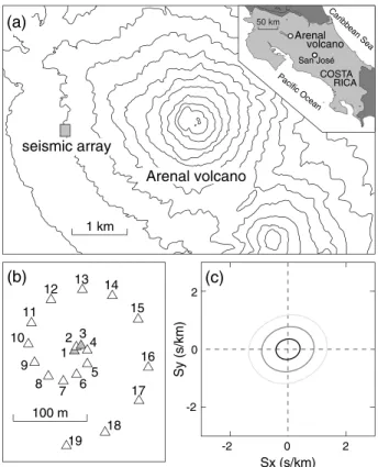
50 km Pacific Ocean Caribbean Sea COSTA RICA Arenal volcano San José

Figure 1. (a) Location of the seismic array about 2 km west of the

Arenal volcano summit. The gray box indicates the array location and corresponds to the area zoomed in Figure 1b. The inset shows the location of Arenal volcano in Costa Rica. (b) Configuration of the seismic array. Grey triangles indicate stations that were partially disre-garded for this study. (c) Beam-forming array response at 2.5 Hz. We show contours of 30, 60, and 90% of the maximum.

activity practically ceased in October 2010, and nowadays, it remains only as a ten-uous degassing. Along the eruption the point of effusion was raised about 250 m from 1974 until 2005 [Wadge et al., 2006] and grew more that 35 m after-ward [Alvarado, 2011], reaching 1750 m asl approximately at the ceasing of the volcanic activity.

Seismic activity accompanying the erup-tion at Arenal until 2010 was characterized by a large variety of signals including har-monic and spasmodic tremors, explosion quakes, LP events, rockfall events, and volcano-tectonic swarms [Alvarado et al., 1997]. Tremors, particularly the harmonic type, and explosion quakes have been the subject of several studies [Alvarado

and Barquero, 1987; Barquero et al., 1992; Alvarado et al., 1997; Benoit and McNutt,

1997; Hagerty et al., 2000; Metaxian et al., 2002; Mora, 2003; Lesage et al., 2006; Davi

et al., 2010, 2012; Almendros et al., 2012],

leading to achieve important advances on the understanding of the source pro-cesses. However, although several source models have been considered, none of them can account for all the features of the seismic signals. More complex has been to match those features to the observations of the volcanic activity and geological context.

Harmonic tremor was the most conspicuous signal at Arenal, usually lasting several hours per day. Har-monic tremor spectra contained several regularly spaced peaks at integer multiples of the fundamental frequency which was generally in the range 0.9–2 Hz [Hagerty et al., 2000; Mora, 2003; Lesage et al., 2006]. Time-frequency analysis of continuous records reveals large variations (>50%) of the fundamental frequency in periods of minutes to tens of minutes [Benoit and McNutt, 1997; Hagerty et al., 2000; Mora, 2003]. Spas-modic tremor was characterized by energy distributed in a wide frequency band, usually in the range 1–6 Hz. Explosion quakes were also quite common, although their number and intensity decreased in the last 10 years of the eruption. Strong explosions were often accompanied by a large audible boom [Alvarado and

Barquero, 1987; Barquero et al., 1992; Garces et al., 1998] producing a high-frequency seismic phase several

seconds after the P wave onset, due to coupling between the acoustic waves and the ground. The explo-sion coda frequently became harmonic tremor [Barquero et al., 1992; Benoit and McNutt, 1997; Hagerty et

al., 2000; Mora, 2003]. LP events were very similar to explosion quakes except that their records had smaller

amplitudes and did not display acoustic phases. Lesage et al. [2006] proposed that LP events and explosion quakes could be considered as part of the same type of event, as there is probably no fundamental differ-ence in their mechanism. In the late 1990s, tens to hundreds of these events were observed each day [Mora, 2003]. The seismic sources of tremor and discrete events were located below the active crater [Alvarado et

al., 1997; Hagerty et al., 2000; Metaxian et al., 2002; Davi et al., 2010, 2012]. Finally, several volcano-tectonic

swarms were usually detected a few months before the major pyroclastic flows originated by crater wall col-lapses [Alvarado and Arroyo, 2000; Alvarado and Soto, 2002]. Other volcano-tectonic swarms were detected during the last stages of the eruption and after the end of volcanic activity.

In this paper, we perform a detailed analysis of LP event and tremor wavefields using data from a dense, small-aperture seismic array operated in 2004. We address their propagation characteristics using two array

2004

1988

1974

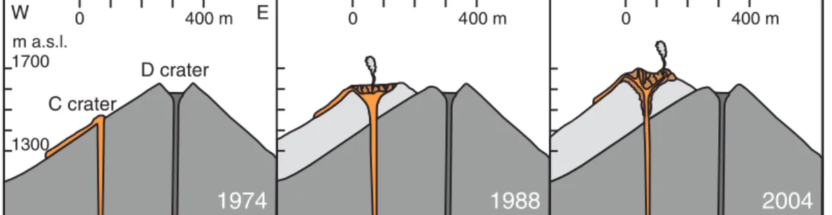
C crater D crater 0 400 m 0 400 m 0 400 m 1300 1700 m a.s.l. W E

Figure 2. Sketch of the plumbing system under the C crater of Arenal volcano at three stages (1974, 1988, and 2004)

during the 1968–2010 eruption. The pre-1968 and post-1968 edifices are shown in dark and light gray, respectively. Fluid magma is represented in orange, while solidified parts are shown in brown.

methods and investigate the similarities and differences in their propagation parameters. We find that LP and tremor wavefields are substantially different, which opposes the widely accepted view of volcanic tremor as a superposition of LP events. We also discuss the detection of multiple simultaneous sources in the seismic wavefield. Our results allow us to propose new insights into the seismic source processes at Arenal volcano, revisiting the interpretation of LP and explosion sources as well as the striking features of harmonic tremors.

2. Instruments and Data

In February 2004 a dense, small-aperture seismic array was deployed during 2.5 days (22 February 01:00 to 24 February 14:00) on the west flank of Arenal volcano, at an elevation of ∼700 m. The summit lies at about 2 km from the array in a 85◦N direction (Figure 1a). The array was composed by 19 short-period (1 Hz), three-component, Lennartz LE-3Dlite seismometers connected to Reftek 130 data loggers recording at a sampling frequency of 100 sps and synchronized by GPS time. Seismometers were distributed in a spiral configuration (Figure 1b) with an aperture of 210 m. It has been demonstrated that the variety of intersta-tion distances that characterizes this configuraintersta-tion reduces the impact of spatial aliasing (S. Gaffet, personal communication, 2003) and generally favors the quality of the array response (Figure 1c).

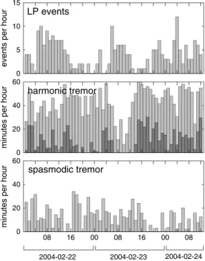
The seismic data recorded during the 60 h of array operations reflect the continuous character of the vol-canic activity at Arenal volcano during the experiment. Although the level of explosions and tremor activity showed a large variability during the eruption, the main spectral features remained similar over time, mak-ing the data set from this short-term experiment quite representative of the overall seismicity of Arenal volcano. The data contain several (∼200) LP events and two types of volcanic tremor (harmonic and spas-modic). Harmonic tremor is the most conspicuous signal, comprising a total of 43 h. On the other hand, spasmodic tremor episodes last for a total of 12 h, part of them overlapped with harmonic tremors. Figures 3 and 4 show examples of the waveforms and spectral contents of these types of signals. Figure 5 shows the temporal distribution of tremors and LP events along the 2.5 days selected for the analysis. The data set contains also a few tectonic earthquakes, but none of them are related to volcanic activity at Arenal. Tremor and LP events can be associated, generating what has been called by Benoit and McNutt [1997] as whooshes and chugs. Lesage et al. [2006] found that there are transitions between harmonic and spasmodic tremor, leading them to propose that a common source can be involved on both harmonic and spasmodic tremor generation. They also reported multiple groups of harmonics in tremor spectrograms, which consti-tute an evidence of simultaneously active sources. Our data contain examples of all these features, such as harmonic tremors with overlapping spectral lines and other evidences of simultaneous sources (Figure 4). In Figure 5 we indicate the temporal extent of this volcanic tremor overlapping.

3. Application of Array Methods

Seismic arrays provide a representation of the propagation of seismic wavefields generated by the volcanic activity. This information can be used both to investigate the peculiarities of the medium and the array sites and to infer the characteristics of the seismogenic processes that occur in volcanoes. Array analyses of volcanic signals have been performed at several volcanic areas such as Kilauea [Goldstein and Chouet,

30000 2004-02-22 01:38:30 10 s 2004-02-23 14:56:10 4000 _{10 s} 2004-02-22 04:25:10 8000 _{10 s} 2 6 10 frequency (Hz) 2 6 10 frequency (Hz) 2 6 10 frequency (Hz)

(a)

(b)

(c)

2

Figure 3. Examples of seismograms and spectrograms of

typ-ical seismovolcanic events: (a) LP event, (b) harmonic tremor, and (c) spasmodic tremor.

1994; Almendros et al., 2001b], Stromboli [Chouet

et al., 1997; La Rocca et al., 2004], Etna [Saccorotti et al., 2004; Di Lieto et al., 2007], Teide [Almendros et al., 2000, 2007], Colima [Palo et al., 2009], Aso

[Takagi et al., 2006], Kirishima [Matsumoto et

al., 2013], and Ubinas [Inza et al., 2014]. These

analyses are specially useful for volcanic tremor, which constitutes an elusive signal that has to be investigated using unconventional approaches. We use array processing techniques to estimate time series of the apparent slowness vectors rep-resentative of the seismic wavefield at Arenal volcano. In order to understand the procedure, we have to underline that the data we are deal-ing with have peculiarities that might complicate the array analysis. For example, we enumerate the following:

1. There are transient (LP events) and sustained signals (volcanic tremor). LP events occur as a response to short-lived perturbations at the seismovolcanic source. The duration of the coherent part (i.e., duration of the source) is shorter than the total duration of the signal (few tens of seconds). Conversely, volcanic tremors are the consequence of a sustained excitation. Although they may display slight fluctuations, they maintain a high level of coherence between array stations for long time spans.

2. Harmonic tremor at Arenal is characterized by important temporal variations in frequency. The fundamental frequency of harmonic tremor is often stable; nevertheless, it can change significantly within minutes (frequency gliding [Lesage et al., 2006]). In any case, tremor frequencies are generally restricted to the 1.5–3.5 Hz range. LP events, on the other hand, have a relatively wide band frequency content. Most energy is contained in the 1–4 Hz band, although their spectra may include relevant energy up to 8 Hz.

3. Multiple sources might be acting simultaneously. This is evidenced by superimposed records of LP and tremors. However, the differences in amplitude and character of these signals are generally large and they can be analyzed independently. A more subtle phenomenon is the activation of multiple har-monic tremor sources at the same time, evidenced by independently evolving sets of harhar-monic lines in the spectrograms.

These peculiarities, specially the last one, constitute a serious challenge for the wavefield analysis capabil-ities of the seismic array. Therefore, we decided to apply two different array methods based on different approaches. The first one is the zero-lag cross-correlation (ZLCC) technique [Frankel et al., 1991; Del Pezzo

et al., 1997]. This is a time domain method that produces highly stable solutions, and within some limits, it

can work with any window length and frequency content. It allows for a robust estimate of the apparent slowness vector of the dominant component of the seismic wavefield. The second method is the multiple signal classification (MUSIC) algorithm [Schmidt, 1986; Goldstein and Archuleta, 1987], a frequency domain technique that stretches the capabilities of array processing in order to enhance resolution in the appar-ent slowness vector plane. MUSIC is limited by the window length, which controls the resolution in time and frequency, like other spectral methods. Above this limitation, the main advantage is that MUSIC allows

2004-02-24 08:23:20 2004-02-23 05:33:20 8000 5000 1 min 1 min 2 6 10 frequency (Hz) 2 6 10 frequency (Hz)

(a)

(b)

Figure 4. Examples of seismograms and spectrograms

reveal-ing double sources: (a) Two simultaneous harmonic tremors and (b) simultaneous harmonic and spasmodic tremors.

for the analysis of complex wavefields containing narrowband signals from several simultaneous sources. In order to make their results compa-rable and aid in the interpretation, we use both methods with similar parameters.

The next step was to check the completeness and quality (signal-to-noise ratio) of the data set. Station 13 did not work for the first 20 h, and a few more stations were intermittently up and down from 12:00 to 14:00 on 22 February. Thus, we do not use these channels at those periods. We have the 19 channels available for 67% of the time, 18 channels for 30% of the time, and 15–17 channels for the remaining 3%. For the ZLCC cal-culations, we rule out two extra stations among those that were tightly deployed in the cen-tral part of the array. Instruments located closer than the distance traveled by the wavefronts at the slowest pace considered (largest apparent slowness) during a sampling interval do not add information to the problem but result in extra noise and worse array response. This precaution is not necessary in the MUSIC method, which works in the frequency domain. We could have stacked the central channels of the array in order to get a single seismogram with improved signal-to-noise ratio (SNR). But there are a few arguments against this, for example: (1) the SNR is good enough for our purposes; (2) for slow waves, stacking could modify substantially the waveforms, since it implies assuming simultaneous arrivals (very small apparent slowness); and (3) interstation distances grow very gradually and it is not clear what stations should be selected. There-fore, we did not stack the seismograms. This processing would make sense if we had low SNR and a set of dense clusters separated by distances much larger than the cluster sizes, as in some large-aperture seismic arrays [Gupta et al., 1990; Rost and Thomas, 2002].

We select the 1–4 Hz band for both analyses. For the ZLCC method, we filter the signals using a zero-phase, two-pole Butterworth filter. For the MUSIC method, we limit the analysis to the spectral values within that range. The low-frequency limit of the frequency band selected is imposed by the instrument response. Although our array is dense enough to make possible the inclusion of frequencies higher than 4 Hz in the analysis, we decided to fix the upper limit to that frequency because of the following reasons: (1) the 1–4 Hz band contains most of the energy of the LP events and tremors; (2) the interpretation of the results is sim-pler when we deal with long wavelengths; and (3) most array methods, and specially MUSIC, work better with narrowband signals.

We adjust the window length for the analysis according to the duration of the input signals. For LP events we selected a 1.28 s (128 samples) window length in order to obtain a good temporal resolution and indepen-dent information for events occurring close in time. In principle there is no limitation on the window length in the ZLCC method, except the recommendation that optimum results for transients are achieved when the window contains two to three cycles at the frequencies of interest [Almendros et al., 1999, 2000]. For the MUSIC method, a trade-off between temporal and spectral resolution has to be achieved. A short window means a sparse spectral representation of the data in the frequency domain. For example, a window of 1.28 s implies that the spectra can be calculated with a frequency interval of 0.78 Hz. Thus, we follow Goldstein

and Archuleta [1991], who suggested the use of a conservative low-frequency limit of twice the frequency

interval, in this case 1.56 Hz. For sustained signals (tremors), we select a window length of 5.12 s (512 sam-ples), which contains about 12 cycles at the central frequency of the band selected. In this way, short-lived transients are averaged and the results reveal mainly the behavior of long-lasting sources. These windows were shifted 0.2 and 0.8 s each step, respectively, to analyze the whole data set.

20 40 60

minutes per hour

20 40 60

minutes per hour

5 10 15

events per hour

08 16 00 08 16 00 08 2004-02-22 2004-02-23 2004-02-24 0 0 0 spasmodic tremor harmonic tremor LP events

Figure 5. Distribution of seismovolcanic signals along

the period analyzed. (a) Hourly number of LP events, (b) minutes of harmonic tremor per hour, and (c) minutes of spasmodic tremor per hour. Dark gray bars in Figure 5b indicate the length of periods with simultaneous sets of independent harmonics.

For each time window, we perform a grid search in the apparent slowness vector space to find the apparent slowness vectors that best repre-sent the propagation properties of the seismic wavefronts. We define an apparent slowness grid from −3.6 to 3.6 s/km in the east and north com-ponents of the apparent slowness vector, wide enough to include the expected range of slow-ness for the signals of interest. The grid spacing was 0.05 s/km, which is adequate to the tem-poral sampling and configuration of the seismic array. For the ZLCC method, we align the seis-mograms for each grid node and calculate the array-averaged cross correlation. The apparent slowness vector corresponding to the maximum average cross correlation (MACC) is regarded as our best estimate of the apparent slowness and azimuth of the wavefield contained in the data window. We define an uncertainty region as the area of the apparent slowness domain where the average cross correlations are larger than 90% of the MACC [Almendros et al., 1999]. For well-correlated signals, the size of this area is sim-ilar to the beam-forming array response shown in Figure 1c. For the MUSIC method, we calcu-late the MUSIC power at each grid node. This magnitude represents the inverse of the projec-tion of the signal vector on the noise subspace [Goldstein and Archuleta, 1987]. Following Ueno

et al. [2010], we fix the signal subspace dimension (number of sources) to 3, given that the sum of the three

largest eigenvalues of the cross-spectral matrix is always above 95% of the total sum of eigenvalues. The apparent slowness vectors corresponding to local maxima in the MUSIC power distribution are regarded as our best estimates of the apparent slowness and azimuths of the wavefield components contained at each window. The corresponding values of peak MUSIC power (PMUP) indicate the relative strengths of these components.

Altogether, the procedure outlined above leads to time series of (1) apparent slowness and propagation azimuth (together with their uncertainties) and (2) a measure of the quality of the solutions (either MACC or PMUP). These outputs represent the direction, velocity, and relative strength of plane wavefronts prop-agating across the array that best fit the real wavefield. In order to extract meaningful information from these apparent slowness vector time series, we use the approach of Almendros et al. [2001b] and focus on the quality and stability of the solutions. Apparent slowness vector data are averaged in short time win-dows comprising either a seismic phase within the LP waveform or a stable section of tremor. Our criteria in selecting these windows are (1) a high PMUP, indicative of good coherence between the array traces, and (2) stability in the back azimuth and apparent slowness estimates. In this way, we obtain a single appar-ent slowness vector estimate for each phase. The total number of estimates is 683 for LP evappar-ents and 3856 for tremor.

4. Results

4.1. LP Events

Although LP events may display a wide range of amplitudes, the array analysis reveals that most of them have similar characteristics in terms of wave propagation. Figure 6 shows examples of the apparent slow-ness vector time series during the onset of three LP events of different sizes. We can identify at least three consecutive phases arriving at approximately fixed time intervals. These phases propagate with similar back

2004-02-23 05:03:54

(a)

(b)

2004-02-22 08:58:01

(c)

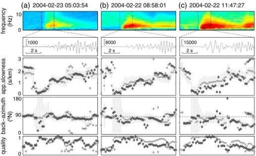
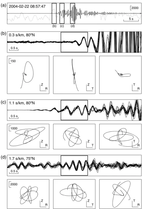
2004-02-22 11:47:27 1000 8000 15000 2 s 2 s 2 s quality back−azimuth (ºN) app.slowness (s/km) 0 1 0 90 180 0 2 1 3 frequency (Hz) 0 10

Figure 6. (a–c) Time series of the apparent slowness vector estimates for three LP events. (from top to bottom)

Spectro-gram, seismoSpectro-gram, apparent slowness, back azimuth, and quality of the estimate (MACC and normalized PMUP). Gray circles show the results of the ZLCC method. Gray and white diamonds correspond to the results of the MUSIC method and represent the dominant and secondary components of the wavefield, respectively. Time labels shown at the top indicate the initial times of the bottom windows (first dashed lines in the spectrograms). Window lengths are 1 min for the top row and 10 s for the remaining rows.

azimuths near 85◦N (coming from the volcano summit direction) and increasing apparent slowness. The event coda is initially incoherent, although it very often evolves into a continuous volcanic tremor. This behavior is common to most LP events throughout the data set.

The first arrival is the fastest and faintest. It propagates across the array site with apparent slowness around 0.4 ± 0.2 s/km. Its amplitude is very small compared to the next phases of the LP event, and thus, we very often miss this arrival for events with low SNR. The second phase is the most coherent. It arrives about 1.5 ± 0.5 s after the first onset, with average apparent slowness around 1.1 ± 0.2 s/km. Very often it has a frequency slightly lower than the remaining waveform. Finally, the last phase arrives about 2.9 ± 0.4 s later, generally displaying the largest seismic amplitudes. It is characterized by a large apparent slowness around 1.7 ± 0.1 s/km and lower coherency.

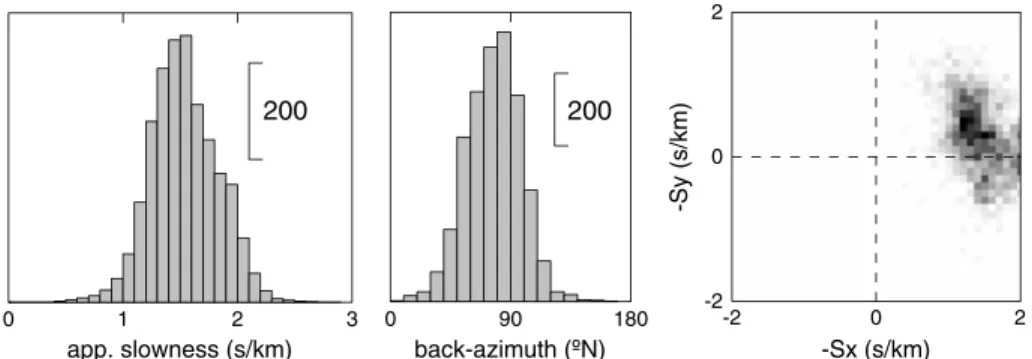
We have not observed a dependence between the apparent slowness vectors, the relative delays of these phases, and the size of the LP events. Furthermore, there are no clear temporal trends either along the time period analyzed. 50 100 app. slowness (s/km) 0 90 180 back-azimuth (ºN) -Sx (s/km) 0 2 -2 2 0 -2 -Sy (s/km) 0 1 2 3

Figure 7. Histograms of the apparent slowness vector results for LP events, obtained using the MUSIC method. (from left

1000 2000 2004-02-22 08:57:47 150

(a)

(b)

(c)

(d)

2000 R Z R Z T Z R T R Z T Z T Z R T R T 5 s 0.5 s 0.5 s 0.5 s (b) (c) (d)

Figure 8. Particle motions for the initial phases of an LP event (shown in Figure 6b). (a) Vertical component seismogram

(black line) and rectilinearity (gray line). Rectilinearity scale ranges from 0 at the bottom of the box to 1 at the top. The three boxes indicate the windows zoomed in Figures 8b–8d. (b, top) Seismograms for all array stations for the first win-dow shown in Figure 8a. Traces have been corrected by propagation delays according to the apparent slowness and back azimuth displayed at the top left. (b, bottom) Particle motion projections in the (left) radial vertical, (center) trans-verse vertical, and (right) radial transtrans-verse planes. (c) Same as Figure 8b; for the second window shown in Figure 8a. (d) Same as Figure 8b; for the third window shown in Figure 8a.

Figure 7 shows a summary of the apparent slowness vector estimates obtained using the MUSIC method for all LP events analyzed. The average back azimuth is 80 ± 10◦. The three peaks in the apparent slowness distribution at 0.4, 1.1, and 1.7 s/km correspond to the three arrivals described above.

We have performed particle motion analyses of the LP events (Figure 8). Following Jurkevics [1988], we correct the array records of propagation delays using the apparent slowness vectors determined by the array analysis. The polarization of the first phase is highly rectilinear. It is contained basically in the inci-dence plane, with dominant vertical motions. This is fully compatible with a P wave propagating with small

(b)

2004-02-23 12:58:20

(a)

2004-02-23 17:56:10

(c)

2004-02-22 01:09:20 quality back−azimuth (ºN) app.slowness (s/km) 0 1 0 90 180 0 2 1 3 frequency (Hz) 0 10 2000 2000 1000 8 s 8 s 8 s

Figure 9. Same as Figure 6 for three samples of volcanic tremor. (a, b) Harmonic tremors and (c) spasmodic tremor.

Window lengths are 5 min for the top row and 40 s for the remaining rows.

apparent slowness. The other two phases have a complex particle motion, with significant energy in the transverse component, suggesting the contribution of surface waves.

4.2. Volcanic Tremor

Figure 9 shows examples of the apparent slowness vector time series during harmonic and spasmodic tremor episodes. The array analysis reveals that harmonic tremors are generally coherent and very sta-ble signals. Nevertheless, the back azimuth estimates are quite diverse for tremors along our data set. For example, Figure 9a corresponds to a signal propagating from ∼120◦N, while Figure 9b displays a signal coming from ∼65◦N. Spasmodic tremors (Figure 9c) show scattered solutions, with generally low values of MACC/PMUP. In fact, only about 5% of the high-quality solutions identified are clearly related to period dominated by spasmodic tremors. In any case, we have observed that there are no fundamental differences among spasmodic and harmonic tremors in terms of propagation azimuths and apparent slowness. Particle motions of volcanic tremor are very complex, with strong transverse components indicative of shear motions. Wave polarization of harmonic tremor is particularly intriguing. The trajectories of the particle motions can be very stable during long time periods. They may show elliptical paths, eight-shaped paths, or even more complex figures. Moreover, they display short-wavelength spatial variations, changing sharply within the array stations over distances of ∼100 m. The investigation of these features exceeds the purpose of the present article and will be the subject of a separate study that is already in preparation.

When we put together all results for volcanic tremor, we find that seismic waves propagate across the array with similar apparent slowness around 1.5 ± 0.3 s/km. There are small variations, but about 90% of the apparent slowness estimates lay between 1 and 2 s/km (Figure 10). The slow propagation and the complex polarization suggest a dominance of surface waves in the seismic wavefield. Contrarily, we find a signifi-cant dispersion in azimuth. This dispersion implies that volcanic tremors may propagate with quite different apparent slowness vectors (i.e., different back azimuths). The average back azimuth for all our tremor esti-mates is 80◦N, which coincides with the back azimuth of the LP events and the direction of the volcano. But there are high-quality estimates of back azimuth in a range of ±40◦from that direction, as illustrated in Figures 9a and 9b. For these estimates, uncertainty regions in the apparent slowness plane subtend angles from the origin of less than 30◦, which gives an indication of the azimuth resolving capabilities of the seis-mic array. Definitely, the array has enough azimuthal resolution to differentiate wave arrivals coming from 40 or 120◦N. We conclude that the scatter in azimuth is not an effect of the array analysis but a real feature of the volcanic tremor wavefields.

200 200 app. slowness (s/km) 0 90 180 back-azimuth (ºN) -Sx (s/km) 0 2 -2 2 0 -2 -Sy (s/km) 0 1 2 3

Figure 10. Same as Figure 7 for apparent slowness vector results corresponding to volcanic tremors.

Large variations in back azimuth are produced even within single-tremor episodes displaying apparently continuous waveforms. For example, Figure 11a illustrates a harmonic tremor episode with apparent slow-ness of ∼2 s/km. Around the center of the time window, we witslow-ness a smooth change in the back azimuth of the wavefield from 50 to 120◦, produced in a time frame of about 10 s. There are no noticeable changes in the frequency of the harmonics. Figure 11b is another example of harmonic tremor, following an LP event, that propagates with apparent slowness of ∼1.5 s/km. In this case, we observe a sharp jump in the back azimuth estimates from 120 to 50◦. Azimuths both before and after the jump remain stable for more than 20 s. In Figure 11c we see both variation styles in a small time frame of about 20 s. At the beginning of the window the back azimuths are stable at 50◦, then they vary smoothly to 120◦, and finally they jump back to 50◦.

In addition to these temporal variations, we have also found clear evidences of multiple, simultaneous wave components in the seismic wavefield (Figure 12). We are able to detect these episodes thanks to the MUSIC capability to provide independent solutions for the coherent wave components present in the wavefield. These episodes of multiple wave components are always related to harmonic tremors, and last a few tens of seconds. They do not occur during spasmodic tremors or LP events, whose wavefields are characterized well enough by a single wave component. In our application we obtain two solutions corresponding to differ-ent appardiffer-ent slowness vectors. The third signal imposed by our selection of the signal subspace dimension is generally characterized by a small PMUP and has not been considered. The differences in the apparent

2004-02-22 02:40:35

(a)

(b)

2004-02-24 04:03:50

(c)

2004-02-23 23:36:05 8 s 8 s 8 s quality back−azimuth (ºN) app.slowness (s/km) 0 1 0 90 180 0 2 1 3 frequency (Hz) 0 10 2000 500 2000 60 s

Figure 11. (a–c) Same as Figure 6 for samples of volcanic tremor with a wavefield displaying varying propagation

2004-02-24 12:05:35

(b)

2004-02-23 11:08:10

(a)

(c)

2004-02-23 14:05:25 quality back−azimuth (ºN) app.slowness (s/km) 0 1 0 90 180 0 2 1 3 frequency (Hz) 0 10 8 s 8 s 8 s 2000 500 1000

Figure 12. Same as Figure 6 for samples of harmonic tremor showing evidences of a complex wavefield. (a) Two

wave-field components at different azimuths, (b) two wavewave-field components with different apparent slowness, and (c) two wavefield components with both different azimuths and different apparent slowness. Window lengths are 5 min for the top row and 40 s for the remaining rows.

slowness vectors of the solutions can be related to propagation azimuth only (Figure 12a), apparent slow-ness only (Figure 12b), or both (Figure 12c). During these multiple source episodes, the PMUP of the secondary peak (which indicates the strength of the secondary component in the wavefield) ranges from small values just above noise level to almost the PMUP of the main peak.

Finally, we have not observed any regular trends in the variations of apparent slowness or back azimuth of volcanic tremor with time.

5. Discussion

5.1. Comparison of Methods

We have applied two array methods (ZLCC and MUSIC) based on different approaches. To our knowledge, this is the first time that a systematic comparison of these methods has been attempted. The combination of results helps us reach a better understanding of the wavefield properties. Generally speaking, the prop-agation azimuths provided by the MUSIC and ZLCC methods coincide, at least within the uncertainty limits of our estimates. On the contrary, the apparent slowness results display slight but systematic variations, specially for harmonic tremors. Figure 13 shows the differences between the back azimuth and apparent slowness values calculated using ZLCC and MUSIC. We include estimates with MACC larger than 0.2 and PMUP over 2, which is not very restrictive (the similarity of results improves when we impose higher thresh-olds). The azimuth distribution is highly peaked near zero, which indicates that both methods produce basically similar back azimuth estimates, as expected. In fact, about 75% of the solutions present differences within ±15◦, which is about the resolution capability of the array for apparent slowness around 1.5 s/km. The apparent slowness distribution is broader and follows a normal distribution. The standard deviation is 0.45 s/km, which is relatively large compared to the resolution capabilities of the array (Figure 1c). The mean is 0.1 s/km, which indicates that for some reason ZLCC tends to produce apparent slowness estimates systematically larger than MUSIC.

This bias may be due to a methodological difference. ZLCC uses directly apparent slowness to calculate interstation delays and align the seismograms. MUSIC uses wave number instead, which is proportional to the product of apparent slowness and frequency. In this algorithm, the apparent slowness values given as results are calculated assuming a “focusing frequency” f0, representative of the signal frequency [Hung and Kaveh, 1988]. Since we use a relatively wide band of 1–4 Hz, the variations in tremor frequency induce

-50 0 50 back-azimuth (º) [cc-mu] -1 0 1 app.slowness (s/km) [cc-mu] normal μ=0 σ=20 Student’s t μ=0 σ=10 ν=2 normal μ=0.1 σ=0.45 10000 10000

Figure 13. Histograms of the differences of

back azimuth and apparent slowness esti-mates provided by the ZLCC and MUSIC methods. Bold lines represent probability dis-tributions with the parameters given: mean (𝜇) and standard deviation (𝜎) for the nor-mal distribution and location (𝜇), scale (𝜎), and degrees of freedom (𝜈) for the Student’s tdistribution.

variations in apparent slowness. The apparent slowness esti-mate SMUfor a signal of frequency f is related to the real

apparent slowness S as follows:

SMU= f f0

S (1)

This implies that MUSIC may underestimate/overestimate the apparent slowness when the frequency of the signal is below/above the focusing frequency. In our case the focusing frequency is 2.54 Hz; thus, the apparent slowness estimates might range from 40% (for 1 Hz) to 160% (for 4 Hz) of the real values. This effect is irrelevant for LP events because of their broadband frequency content, but it might be significant for harmonic tremors. The comparison with the ZLCC estimates allows us to detect the occurrence of this effect.

Notice that the apparent slowness shown along the paper are the raw estimates obtained with MUSIC and ZLCC. MUSIC results for harmonic tremors have not been corrected by the effect of the difference between the fundamental frequency and the focusing frequency, described above. This correction might vary slightly the actual values of apparent slowness, which would be increased for low-frequency signals and decreased for high-frequency signals. Most part of the har-monic tremors have fundamental frequencies in the 2–2.5 Hz range, which would explain the slight difference between the ZLCC and MUSIC estimates. In any case, the differences are not large enough to modify our interpretation of the results. On the other hand, the ZLCC method is not designed for multiple wavefield components. Yet it is some-what able to detect their presence when the apparent slowness vectors are different enough. For example, when two wave components propagate with different azimuths, ZLCC provides solutions that jump from one to the other (Figures 12a and 12c). The method is less sensitive to changes in apparent slowness, and when waves with different apparent slowness are involved, it yields a single solution between the apparent slowness provided by MUSIC (Figures 12b and 12c). In general, all these solutions have low MACC values. Figure 14 shows a detailed view of what the array sees during one of these intervals with multiple wavefield components. The distributions of average cross correlation and MUSIC power correspond to a period at the center of Figure 12a. Initially, there is a single peak with back azimuth of ∼50◦N and apparent slowness of ∼2 s/km. Later, we notice the appearance of a secondary peak with back azimuth of ∼100◦N and similar apparent slowness that eventually becomes dominant. MUSIC is able to identify both signals; however, ZLCC provides either one or the other.

5.2. LP Events

Our results indicate that LP events display three phases with similar propagation azimuths and increas-ing apparent slowness. The back azimuths of these three phases are 80±10◦, which coincide with the array-crater direction of 85◦N. On the contrary, the three phases have different behaviors in terms of appar-ent slowness. The first phase is a faint arrival characterized by a small apparappar-ent slowness of 0.4 s/km and a linear polarization in the incidence plane, implying near-vertical incidence of body waves, i.e., P waves. There is a second phase with intermediate apparent slowness of 1.1 s/km, followed by a third phase with high apparent slowness of 1.7 s/km. The large apparent slowness and the complex particle motions point to the presence of surface waves. Both late phases display large amplitudes, specially the third one. The delays of the second and third phases relative to the first are about 1.5 and 4.4 s.

Our interpretation of these apparent slowness vector results in terms of source position and characteris-tics is limited basically by the use of a single seismic array and our poor knowledge of the seismic velocity structure. Single-array source locations rely on a proper representation of wave propagation through the medium [Goldstein and Chouet, 1994; Almendros et al., 1999; Ibá˜nez et al., 2003], and thus, they are severely

Sx(s/km) -2 0 2 11:08:32.3 11:08:36.3 11:08:28.3 11:08:24.3 Sx(s/km) -2 0 2 Sy(s/km) -2 0 2 Sy(s/km) -2 0 2 CC MU Sx(s/km) -2 0 2 Sx(s/km) -2 0 2

Figure 14. Distributions of (top row) MUSIC power and (bottom row) average cross correlation in the apparent slowness

vector plane during a change in the dominant component of the harmonic tremor wavefield at about 11:08:30 on 23 February 2004.

affected by uncertainties in the velocity model. On the other hand, multiple arrays allow for quantitative estimates of source locations [Almendros et al., 2001a, 2001b; Metaxian et al., 2002; La Rocca et al., 2004;

Saccorotti et al., 2004; Di Lieto et al., 2007; Ryberg et al., 2010; Inza et al., 2014].

Although we cannot determine precisely the source location, we can use our apparent slowness and back azimuth results to constrain the source region of LP events. Taking into account the coincidence of the LP back azimuths with the direction to the volcano summit, we assume that LP epicenters are likely located in the crater area. For a fixed epicentral distance, the apparent slowness of a body wave generally decreases with increasing source depth. Thus, the small apparent slowness of the P wave might suggest that LP events originate in a relatively deep source. Nevertheless, the apparent slowness of a seismic phase depends not only on the source depth but on the velocity structure of the medium as well. An adequate interpretation of apparent slowness in terms of source depth requires some knowledge of the velocity structure.

The velocity structure of Arenal volcano has been investigated by Mora et al. [2006]. They performed refrac-tion surveys on the east and west flanks of the volcano and applied the spatial autocorrelarefrac-tion (SPAC) method to calculate velocity models under two small-aperture, semicircular arrays. One of these models coincides with our array site. The model contains very slow and very thin shallow layers that may affect crit-ically seismic wave propagation (e.g., Vp is 300 m/s for the first 3 m). In any case, Mora et al. [2006] shows that the structure of Arenal is complex and varies in length scales smaller than 100 m. For low-frequency signals, the involved wavelengths are larger than the layer thicknesses, and thus, we cannot rely on ray the-ory to image the seismic wave behavior. Full-wavefield numerical simulations are required to understand wave propagation.

Metaxian et al. [2009] performed wave propagation simulations in a 3-D model of Arenal volcano

includ-ing topography. They combined the velocity models of Mora et al. [2006] to define a general model that could be useful for low-frequency signals. This model has two layers with thicknesses of 100 and 250 m and

Pwave velocities of 2.0 and 2.5 km/s, over a half-space with P wave velocity of 3.5 km/s. Layer interfaces fol-low the topography. Metaxian et al. [2009] used a 3-D elastic lattice approach [O’Brien and Bean, 2004] to generate the seismic wavefield recorded by a set of 35 nine-receiver seismic antennas distributed in a grid around the volcano at distances up to 8 km. They estimated the apparent slowness vectors at these arrays using the method of Metaxian et al. [2002] for different source locations and mechanisms. Their results show that for a source located at a depth of about 500 m beneath the crater, the synthetic array closest to our array site measures back azimuths pointing to the crater, with a slight northward deviation related to topography. Apparent velocities measured for the synthetic wavefields are 2–3 km/s. These velocity val-ues correspond to apparent slowness of 0.3–0.5 s/km, which coincide with the range we observe for the P waves. Using these results, we conclude that our apparent slowness estimates could be fully compatible with a source located at shallow depths (<500 m) below the summit.

Moreover, our results show that the second and specially the third LP phases have large apparent slowness, which suggests that they are most likely composed of surface waves. And, remarkably enough, they have also large amplitudes, indicating a significant contribution of surface waves to the LP event waveform. A deep source is not an efficient generator of surface waves. The dominant presence of surface waves in the LP events also supports their origin in a shallow source.

This conclusion agrees with most studies of LP events at Arenal volcano that hint to a shallow source located a few hundred meters below the summit craters [Alvarado et al., 1997; Hagerty et al., 2000; Lesage et al., 2006;

Davi et al., 2010; Valade et al., 2012]. Explosion quakes with acoustic phases are assumed to be very shallow,

while LP events are slightly deeper [Valade et al., 2012]. These conclusions are supported by considerations about the characteristics of the acoustic source [Benoit and McNutt, 1997; Garces et al., 1998] and are consis-tent with most of the observations. For example, Hagerty et al. [2000] analyzed LP events recorded between 1995 and 1997 with a five-station seismic network and a linear array deployed at Arenal volcano. They iden-tified three phases in the LP onset and were able to measure apparent velocities at the array. These phases propagated at about 3.0, 1.3, and 0.6 km/s, corresponding to apparent slowness of 0.3, 0.8, and 1.7 s/km that are compatible with our results. Hagerty et al. [2000] interpreted the emergent, low-amplitude phase as a P wave; the second, more energetic phase as S wave energy; and the third phase as surface waves traveling within the shallow unconsolidated layers of the volcano edifice. They reported a delay of 1.0 ± 0.3 s between the P and S phases. Furthermore, they used P wave arrival times and a homogeneous half-space with P wave velocity of 2.5 km/s to locate the LP sources. The results point to a source region located at a depth of ∼2 km below the summit. However, further analyses and comparisons of the relative timing between seismic and acoustic waveforms of explosion quakes led them to suggest that the seismic source should be much shal-lower. Metaxian et al. [2002] deployed four seismic arrays around Arenal volcano in 1997, at distances from the summit between 2 and 3.8 km. They performed a geometrical joint location [Almendros et al., 2001a] using back azimuth estimates of LP events and explosion quakes. Their results show that the epicenters are located in the crater area, within 400 m of the active crater. Finally, Davi et al. [2010] used data from a nine-station broadband network deployed in 2005 to perform a moment tensor inversion of an LP event. They searched for the most likely point source location and mechanism and concluded that the LP wave-form is adequately represented by an isotropic explosion located at very shallow depths below the crater (∼200 m).

The timing of the LP phases following the P wave is another constraint that must be met. In this case, the simulations of Metaxian et al. [2009] do not coincide with the observations. If we interpret our second LP phase as S wave energy [Hagerty et al., 2000], then the observed delay between the P and S phases is ∼1.5 s. This value triplicates the predicted delay of ∼0.5 s for a source at 500 m depth below the craters. The situ-ation is even worst for the surface waves reaching the array 4.4 s after the P wave. These values seem too large for a source located at an epicentral distance of 2 km. It is likely that the shallow, unconsolidated layers of the volcano edifice play an important role in the large delays observed. A more detailed velocity model of Arenal volcano would be required to reproduce the observed delays of the seismic phases.

5.3. Volcanic Tremor

The analysis of the volcanic tremor wavefield reveals that spasmodic tremor is an incoherent signal that cannot be simply fitted by plane wavefronts. On the contrary, harmonic tremor is highly coherent. Appar-ent slowness values range mostly between 1 and 2 s/km. Propagation azimuths are variable, covering a broad span up to ±40◦from the crater-array direction. There is a significant dispersion in the solutions cor-responding to different volcanic tremor episodes, especially in back azimuth. Changes in back azimuth are also observed within single-tremor episodes.

The large apparent slowness and the complex particle motions suggest that volcanic tremor at Arenal is composed of a mixture of surface waves. This coincides with observations of the seismic wavefield at other volcanic areas [e.g., Almendros et al., 1997; Metaxian et al., 1997; Chouet et al., 1998; Konstantinou and

Schlindwein, 2002; Saccorotti et al., 2001, 2004; Ibá˜nez et al., 2008]. The range of apparent slowness of 1–2

s/km corresponds to apparent velocities between 0.5 and 1.0 km/s. Mora et al. [2006] analyzed data from a seismic array deployed at the same location we have used in this work and found a dispersion curve for Rayleigh waves with phase velocities of 0.95, 0.76, and 0.56 km/s for 1, 2, and 4 Hz, respectively. These val-ues fall within the apparent velocity range determined by our array, which indicates that surface waves dominate the tremor wavefield.

frequency (Hz) back−azimuth (deg) 1 2 3 4 30 90 150 frequency (Hz) app.slowness (s/km) 1 2 3 4 0 1 2 3

Figure 15. Distributions (2-D histograms) of back azimuth and

appar-ent slowness versus fundamappar-ental frequency for harmonic tremors. We use∼38,500 simultaneous estimates of apparent slowness vectors and tremor frequencies obtained along the data set. The color scale ranges from 0 (white) to 1700 (black). The dashed line indicates the approximate position of the dispersion curve determined by Mora et al. [2006].

In spite of this coincidence, we have not found evidences of surface wave dis-persion. In principle, harmonic tremors with different fundamental frequencies would sample the medium to different depths, and thus, they should propa-gate with phase velocities that decrease with increasing tremor frequency. We have used the semiautomated method of

Lesage [2009] to measure the fundamental

frequency of harmonic tremors along the data set. We assign the apparent slowness vectors corresponding to the main peak of the MUSIC spectra to these fundamen-tal frequencies. The resulting distributions (Figure 15) indicate that the range of apparent slowness coincides with the val-ues obtained by Mora et al. [2006]. It is also clear that the apparent slowness of harmonic tremor shows only a very loose correlation with frequency, even if we correct the MUSIC estimates of apparent slowness for the effect of the difference between the signal frequency and the focusing frequency. The scatter of solutions is too large, which might indicate the occurrence of other processes masking the effect of surface wave dispersion.

The location of the volcanic tremor source is a difficult task that has to be approached with unconventional techniques such as array analyses [Metaxian et al., 1997; Almendros et al., 1999, 2001a, 2001b; La Rocca et

al., 2004], seismic amplitude distributions [Battaglia and Aki, 2003; Battaglia et al., 2005; Patane et al., 2008; Haney, 2010], moment tensor inversions [Davi et al., 2012], and time reversal imaging [Lokmer et al., 2009].

Attempts to determine the position of the volcanic tremor source at Arenal volcano suggest that it is located at shallow depths beneath the craters, basically coinciding with the source of the LP events. For exam-ple, Metaxian et al. [2002] used a probabilistic source location approach based on back azimuth estimates obtained with multiple seismic arrays deployed around the volcano. They analyzed a set of 45 records of volcanic tremor and found that the most likely epicenter locations clustered within 600 m of the summit craters. Davi et al. [2012] used an approach based on moment tensor inversions of the tremor waveforms. They found that the most likely source mechanism is a subhorizontal crack located within a few hundred meters of the active crater. Source depth is estimated to be just ∼100 m.

Apart from these direct estimates, investigations of the source process of harmonic tremor yield pressure ranges compatible with a shallow source under the crater [Benoit and McNutt, 1997; Garces et al., 1998;

Hagerty et al., 2000; Lesage et al., 2006].

These results raise an interesting question. If the source is indeed located in a shallow volume beneath the volcano summit, then why do we retrieve such a wide span of tremor back azimuths? We observe back azimuths from 40 to 120◦N for different tremor episodes. Moreover, we find temporal changes dur-ing apparently stable harmonic tremors, includdur-ing both rapid jumps and smooth variations in scales of tens of seconds. These results seem to suggest the presence of an extended source region. The activation of different parts of this source would produce tremors with different propagation azimuths. Jumps in the propagation parameters would be produced by the alternate activation of two different sections of the extended source, situated at different positions within the volcano. Gradual variations would respond to the horizontal displacement of the active section of the conduits where tremors are generated. However, the magnitudes of the variations observed in the propagation azimuths amount to many tens of degrees. This result seems to imply an unrealistically large source extent of the order of the source-array distance, which is incompatible with a shallow tremor source at the volcano summit.

Nevertheless, we must consider that seismic wavefields propagating in a heterogeneous medium may be subject to important distortions. These distortions are particularly noticeable at volcanoes, generally charac-terized by heterogeneous velocity structures and rough topographies. Wave propagation effects have been investigated at several volcanoes, for example, using active source experiments [La Rocca et al., 2001; Nisii

et al., 2007; Garc´ıa-Yeguas et al., 2011] and numerical simulations [Almendros et al., 2001a; Bean et al., 2008; O’Brien and Bean, 2009; Metaxian et al., 2009; Kumagai et al., 2011]. These results indicate that propagation

azimuths may deviate up to several tens of degrees from the source-receiver direction, even in short dis-tances. Thus, a back azimuth estimate is not directly interpretable in a geometrical sense as pointing straight back to the source. In our case, it is likely that the heterogeneity of the velocity structure of Arenal volcano and its rough topography produce important distortions in the seismic wavefield. In particular, tremor wave-fields would be most sensitive to propagation effects, since they are mainly composed of surface waves that propagate within the shallowest, most heterogeneous layers of the volcano.

The image that emerges is that of a complex source region with small-scale heterogeneities generating a variable seismic radiation pattern and complex propagation effects producing lateral deviations of the seismic wave paths. Given that in general the medium does not change significantly its properties in short time scales, a perfectly stationary source would produce waves propagating across the array from a def-inite direction. It might not coincide with the source-array direction due to path effects, but it would be constant throughout the data set. Thus, the processes ultimately responsible for the azimuth variability of volcanic tremor must occur within the source region. This region located at shallow depths below the vol-cano summit is the locus of highly dynamic energy exchanges between the magma mix, the solid rock, and the atmosphere. It is subject to rapidly changing physical conditions that may affect the location, depth, and even the mechanism of the tremor-generating processes.

Evidences of changing conditions in the source region are described by Valade et al. [2012]. They compared seismic data and Doppler radar measurements of pyroclastic emissions obtained at Arenal volcano in 2005. These data allowed them to investigate the relationship between gas and tephra emissions. They found a very poor correlation between the occurrence and characteristics of seismic activity and tephra emissions imaged by radar. To explain this striking observation, Valade et al. [2012] proposed a conceptual model where the shallow system properties (plug thickness, rheology, fracturing, and permeability) are utterly vari-able, thus yielding nonrepeatable conditions that may account for the disconnection between radar and seismic signals.

The volcano edifice limits the horizontal extent of a shallow source region to a radius of a few hundred meters. This size could be enough to explain our observations, provided that important path effects take place. Small variations in the source position, depth, or mechanism may produce large differences in the path followed by the seismic waves. For example, we could imagine a low-velocity zone between the source and the array, producing a “lens effect.” This geometry was discussed by Garc´ıa-Yeguas et al. [2011] in their interpretation of the apparent slowness vectors observed during an active source experiment at Deception Island volcano. Waves originating in the north part of the source region would be deflected southward and arrive at the array site with a counterclockwise rotation of the apparent slowness vectors, as compared to the source-array direction. Similarly, waves originating in the south of the source region would be deflected northward (clockwise rotation of the apparent slowness vector). Another structure that could be consid-ered is the interface between the pre-1968 and post-1968 edifices at Arenal volcano. Lindquist et al. [2007] analyzed the bias in the apparent slowness vector estimates produced by a dipping Moho discontinuity beneath a medium-aperture seismic array located in Alaska. They concluded that this discontinuity pro-duced deviations in azimuth that depend on the source position relative to the dipping layer. For a flat surface, the magnitude of the deviations as a function of source back azimuth follows a cosine function. Maximum deviations of ∼10◦occur for sources located in directions that parallel the strike of the dipping interface. Although the scales are different, and the interface between the pre-1968 and post-1968 edifices is not flat, these results could indicate that the old cone discontinuity might bear an important weight in the observed spreading of the tremor back azimuth estimates.

We conclude that propagation effects due to the topography and heterogeneous velocity structure could be able to amplify the small changes that occur within the source volume, thus yielding the wide span of back azimuths observed. In this interpretation, the variability of the tremor back azimuths reflects the coupled effect of changing conditions at the source and heterogeneity of the velocity structure.

5.4. Simultaneous Harmonic Tremor Sources

On top of the complexity of the volcanic tremor wavefields described above, we have found that in several periods our results hint to the presence of multiple, simultaneous harmonic tremors in the seismic wavefield of Arenal volcano. Evidences are: (1) the visual identification in the spectrograms of multiple, simultaneous

groups of harmonics that evolve independently, (2) the development of complex spatial amplitude pat-terns related to wave interference, and (3) the appearance of multiple apparent slowness vectors in the MUSIC solutions.

The first indication of simultaneous tremor sources is the observation of multiple sets of harmonics in the spectrogram of harmonic tremor, which evolve independently (e.g., Figure 4). Simultaneous sets of harmon-ics at Arenal volcano have been described by Lesage et al. [2006]. They analyzed the spectral behavior of harmonic tremors and concluded that at some periods two sources were active within the volcano. Lesage

et al. [2006] also reports the simultaneous observation of gas emissions from two active vents, which

sup-ports their interpretation. Resup-ports of harmonic tremors with multiple sets of harmonics are indeed very rare in the literature, which emphasizes the interest of the present analysis. Apart from Arenal, we could find just one description of multiple sets of harmonics in the seismic signals associated to large icebergs [Aster et al., 2004]. However, this kind of behavior is quite common in our data set (Figure 5).

The second indication comes from the analysis of the seismic amplitudes at the array stations. Almendros

et al. [2012] used our same data set to describe the anomalous behavior of the harmonic tremor amplitudes

observed at the seismic array. They found strong variations among the amplitudes of sustained harmonic tremors recorded at the different array stations. The resulting amplitude patterns were geometrically com-plex, they were stable over periods of a few tens of seconds but changed with time on longer time scales, and they were related solely to harmonic tremors and disappeared when any other type of seismicity dominated the wavefield. Almendros et al. [2012] interpreted these complex amplitude patterns as a result of wave interference among different signals composing the harmonic tremor wavefield. Thus, we propose that the complexity of the spatial distribution of tremor amplitudes might indicate the simultaneous activation of multiple tremor sources.

Finally, the third indication comes from the results of our array analysis of the tremor wavefield. The applica-tion of the MUSIC algorithm to harmonic tremors sometimes produces two high-PMUP estimates indicating the presence of two significant wave components with different propagation properties (Figure 12). The dif-ferences may occur in apparent slowness, back azimuth, or both. Harmonic tremor wavefields are generally characterized by apparent slowness in the range 1–2 s/km. Whenever MUSIC provides two solutions with different apparent slowness, one of the components has an apparent slowness of 0.5–1.5 s/km while the other has a large apparent slowness of 2–3 s/km (Figure 12). These slownesses are of the same order as the slowness of sound in the air and suggests a link with the propagation of acoustic waves in the atmosphere. In other instances there are large differences in the back azimuths, and none of them point directly to the crater. This observation is difficult to reconcile with a single-tremor source located at the volcano summit. However, as discussed above, it could be explained by the combination of a complex source region with multiple active sections and strong propagation effects due to the topography and heterogeneous shallow structure of the volcanic medium.

We have reviewed the occurrence of these three wavefield characteristics in our data set to investigate the presence of multiple, simultaneous tremor sources. We presume that these effect should be some-how related, since all of them are evidences of a dual tremor source. Figure 16 ssome-hows the spectrograms, average amplitudes, and back azimuth estimates of harmonic tremors corresponding to different periods. Figures 16a–16d are samples of harmonic tremor whose spectrograms show a single set of harmonics. On the contrary, Figures 16e and 16f display spectrograms where two different sets of harmonics evolving independently can be clearly identified, thus suggesting a double tremor source. Figures 16a–16c show harmonic tremors with strong differences of seismic amplitude among array stations, originated by the interference of two wavefield components. On the contrary, Figures 16d–16f display harmonic tremors with similar amplitudes at all stations. Average amplitudes are measured using the RMS of the seismic waveform in 10 s long windows [Almendros et al., 2012]. Figures 16b, 16d, and 16f illustrate the clear detection of two wavefield components with different back azimuths. On the contrary, Figures 16a and 16e correspond to a wavefield with a single, dominant wavefield component.

From these plots, we find that there is no clear relationship between the presence of multiple sets of har-monics, a complex amplitude pattern, and MUSIC detection of two wavefield components. In fact, these effects can appear alone while the other two are absent, as revealed by Figures 16a (amplitude pattern), 16d (dual MUSIC solutions), and 16e (two sets of harmonics). Figure 16b shows both amplitude differences and two MUSIC solutions. Figure 16f shows both a double set of harmonics in the spectrogram and two MUSIC

2004-02-23 19:26:00

(a)

back−azimuth (ºN) 0 90 180 frequency (Hz) 0 10 5 15 station# 2004-02-23 19:26:50

(b)

(c)

2004-02-23 02:03:30 2004-02-24 06:06:05 (d) (e)2004-02-24 07:53:25 (f) 2004-02-24 08:27:40 back−azimuth (ºN) 0 90 180 frequency (Hz) 0 10 5 15 station# 8 s 8 s 8 s 8 s 8 s 8 s 60 s 60 s 60 s 60 s 60 s 60 s 0.3 0.5 0.7 0.9 RMS / max(RMS)

Figure 16. (a–f ) Comparison among evidences of multiple harmonic tremor sources. We show, from top to bottom, the

spectrogram, color-coded average amplitude versus time at each array station, and back azimuth estimates. The time label indicates the start of the back azimuth time window. Window lengths are 5 min for the top and middle rows and 40 s for the bottom row.

solutions. The only combination that seems incompatible is the simultaneous occurrence of two sets of harmonics and a complex amplitude pattern at the array.

The complex spatial amplitude patterns usually occur during clean, relatively stable sections of harmonic tremor, as already noticed by Almendros et al. [2012]. They do not occur when multiple sets of harmonics crisscross in the spectrogram. Almendros et al. [2012] proposed that the amplitude patterns at the array are produced by interference of two wavefield components. If this is the case, the presence of these two inter-fering signals is not evident from the spectrograms. The reason we cannot see them could be that the two wave components have different apparent slowness vectors but similar frequencies. Almendros et al. [2012] showed that the positions of the crests of the interference pattern of two plane waves are related to the difference of frequency between them. When the waves have the same frequency, the pattern is station-ary. When the waves have different frequencies, the patterns evolve with time. Our method to identify the occurrence of complex amplitude patterns is based on the measure of the average wave amplitudes in 10 s long windows [Almendros et al., 2012]. Thus, we may fail to detect them if the amplitude ratios vary on time scales much shorter than 10 s. That is, we cannot detect a clear interference pattern unless the difference of frequencies is smaller than 0.1 Hz.

In summary, all these observations indicate that harmonic tremors are highly complex signals. They result from time-varying single or double sources. The precise wave propagation paths in the hetero-geneous medium depend critically on the location and characteristics of the source. The combination of strong source and path effects produces the variety of features revealed by the spectral, array, and amplitude analyses.

5.5. Relationship Between LP Events and Tremor

At many volcanoes around the world, LP events and volcanic tremor are intimately linked. They usually share similar spectral characteristics, source locations, wave propagation parameters, etc [Almendros et al., 1997;