HAL Id: tel-01982622
https://tel.archives-ouvertes.fr/tel-01982622
Submitted on 15 Jan 2019
HAL is a multi-disciplinary open access
archive for the deposit and dissemination of sci-entific research documents, whether they are pub-lished or not. The documents may come from teaching and research institutions in France or abroad, or from public or private research centers.
L’archive ouverte pluridisciplinaire HAL, est destinée au dépôt et à la diffusion de documents scientifiques de niveau recherche, publiés ou non, émanant des établissements d’enseignement et de recherche français ou étrangers, des laboratoires publics ou privés.
Canopy height estimation on a regional scale :
Application to French Guiana
Ibrahim Fayad
To cite this version:
Ibrahim Fayad. Canopy height estimation on a regional scale : Application to French Guiana. Signal and Image processing. Université Montpellier, 2015. English. �NNT : 2015MONTS143�. �tel-01982622�
THESE DE DOCTORAT
DE L’UNIVERSITE DE MONTPELLIER
Spécialité
Systèmes Automatiques et Microélectroniques (SYAM) (Ecole Doctorale: Information, Structures, Systèmes)
Présentée par
Ibrahim FAYAD
Pour obtenir le grade de
Docteur de l’Université de Montpellier
ESTIMATION DE LA HAUTEUR DES ARBRES
A L
'
ECHELLE REGIONALE
:
APPLICATION A
LA GUYANE FRANÇAISE
Soutenue le 15/06/2015, devant le jury composé de :
Dr. Patrick Chazette
Ingénieur-chercheur, CEA, Rapporteur
Dr. Xavier Briottet
Directeur de recherche, Onera, Examinateur
Dr. Nicolas Baghdadi
Directeur de recherche, Irstea, Directeur de thèse
Dr. Grégoire Vincent
Chargé de recherche, IRD, Rapporteur
Dr. Mehrez Zribi
Directeur de recherche, CNRS, Examinateur
Dr. Nicolas Barbier Chargé de recherche, IRD, Co-directeur de thèse
A
BSTRACT
Remote sensing has facilitated the techniques used for the mapping, modeling and understanding of forest parameters. Remote sensing applications usually use information from either passive optical systems or active radar sensors. These systems have shown satisfactory results for estimating, for example, aboveground biomass in some biomes. However, they presented significant limitations for ecological applications, as the sensitivity from these sensors has been shown to be limited in forests with medium levels of aboveground biomass. On the other hand, LiDAR remote sensing has been shown to be a good technique for the estimation of forest parameters such as canopy heights and above ground biomass. Whilst airborne LiDAR data are in general very dense but only available over small areas due to the cost of their acquisition, spaceborne LiDAR data acquired from the Geoscience Laser Altimeter System (GLAS) have low acquisition density with global geographical cover. It is therefore valuable to analyze the integration relevance of canopy heights estimated from LiDAR sensors with ancillary data (geological, meteorological, slope, vegetation indices etc.) in order to propose a forest canopy height map with good precision and high spatial resolution. In addition, estimating forest canopy heights from large-footprint satellite LiDAR waveforms, is challenging given the complex interaction between LiDAR waveforms, terrain, and vegetation, especially in dense tropical and equatorial forests. Therefore, the research carried out in this thesis aimed at: 1) estimate, and validate canopy heights using raw data from airborne LiDAR and then evaluate the potential of spaceborne LiDAR GLAS data at estimating forest canopy heights. 2) evaluate the fusion potential of LiDAR (using either sapceborne and airborne data) and ancillary data for forest canopy height estimation at very large scales. This research work was carried out over the French Guiana.
The estimation of the canopy heights using the airborne dataset has been carried out using a simple algorithm, which first extracts the canopy top and ground points, and then interpolates the canopy height using the ground point and its surrounding canopy top points. Results indicated an RMSE on the canopy height estimates of 1.6 m. Next, the potential of GLAS for the estimation of canopy heights was assessed using multiple linear (ML) and Random Forest (RF) regressions using waveform metrics and principal component analysis (PCA). Results showed canopy height estimations with similar
precisions using either LiDAR metrics or the principal components (PCs) (RMSE ~ 3.6 m). However, a regression model (ML or RF) based on the PCA of waveform samples is an interesting alternative for canopy height estimation as it does not require the extraction of some metrics from LiDAR waveforms that are in general difficult to derive in dense forests, such as those in French Guiana.
Next, canopy heights extracted from both airborne and spaceborne LiDAR were first used to map canopy heights from available mapped environmental data (geological, meteorological, slope, vegetation indices etc.). Results showed an RMSE on the canopy height estimates of 6.5 m from the GLAS dataset and of 5.8 m from the airborne LiDAR dataset. Then, in order to improve the precision of the canopy height estimates, regression-kriging (regression-kriging of random forest regression residuals) was used. Results indicated a decrease in the RMSE from 6.5 to 4.2 m for the regression-kriging maps from the GLAS dataset, and from 5.8 to 1.8 m for the regression-kriging map from the airborne LiDAR dataset. Finally, in order to study the impact of the spatial sampling of future LiDAR missions on the precision of canopy height estimates, six subsets were derived from the airborne LiDAR dataset with flight line spacing of 5, 10, 20, 30, 40 and 50 km (corresponding to 0.29, 0.11, 0.08, 0.05, 0.04, and 0.03 points/km², respectively).
Results indicated that using the regression-kriging approach, the precision on the canopy height map was 1.8 m with flight line spacing of 5 km and decreased to an RMSE of 4.8 m for the configuration for the 50 km flight line spacing.
RESUME
La télédétection contribue à la cartographie et à la modélisation des paramètres de la forêt. Ce sont les systèmes optiques et radars qui sont le plus généralement utilisés pour extraire des informations utiles à la caractérisation des paramètres forestiers. Ces systèmes ont montré des résultats satisfaisants pour estimer, par exemple, la biomasse dans certains biomes. Cependant, ils présentent des limitations importantes pour des forêts ayant un niveau de biomasse élevé. En revanche, la télédétection LiDAR s’est avérée être une bonne technique pour l'estimation des paramètres forestiers tels que la hauteur de la canopée et la biomasse. Alors que les LiDAR aéroportés acquièrent en général des données avec une forte densité de points mais sur des petites zones en raison du coût de leurs acquisitions, les données LiDAR satellitaires acquises par le système spatial (GLAS) ont une densité d'acquisition faible mais avec une couverture géographique mondiale. Il est donc utile d'analyser la pertinence de l'intégration des hauteurs estimées à partir des capteurs LiDAR et des données auxiliaires (géologiques, météorologiques, pente, indices de végétation, etc.) afin de proposer une carte de la hauteur des arbres avec une bonne précision et une résolution spatiale élevée. En outre, l'estimation de la hauteur des arbres à partir des formes d’onde GLAS avec ses grandes empreintes est difficile compte tenu de l'interaction complexe entre les formes d'onde LiDAR, le terrain et la végétation, en particulier dans les forêts tropicales et équatoriales denses. Par conséquent, la recherche menée dans cette thèse vise à: 1) Estimer et valider la hauteur des arbres en utilisant des données acquises par des LiDAR aéroportés et satellitaire (capteur GLAS). 2) évaluer le potentiel de la fusion des données LiDAR (avec les données aéroportées ou satellitaires) et des données auxiliaires pour l'estimation de la hauteur des arbres à une échelle régionale. Ce travail de recherche a été effectué sur la Guyane française.
L'estimation de la hauteur des arbres en utilisant les données aéroportées a été réalisée en utilisant un algorithme simple, qui extrait d'abord les points haut de la canopée et ceux du sol, puis interpole la hauteur de la canopée en utilisant les points du sol et les points hauts de la canopée. Les résultats ont indiqué une EQM sur les estimations de la hauteur de la canopée de 1,6 m. Ensuite, le potentiel de GLAS pour l'estimation de la hauteur des arbres a été évalué en utilisant des modèles de régression linéaire (ML) ou Random Forest (RF) avec des métriques provenant de la forme d'onde et de l'analyse en composantes principales
(ACP). Les résultats ont montré que les modèles d’estimation des hauteurs des arbres avaient des précisions semblables en utilisant soit les métriques LiDAR ou les composantes principales (PC) (EQM ~ 3,6 m). Toutefois, un modèle de régression (ML ou RF) basé sur les composantes principales obtenues à partir des formes d’onde GLAS est une alternative intéressante pour l'estimation de la hauteur des arbres, car il ne nécessite pas l'extraction de certaines métriques à partir des formes d'onde LiDAR qui sont en général difficiles à dériver dans les forêts denses, telle que la Guyane française.
Finalement, la hauteur des arbres extraite à la fois des données LiDAR aéroporté et GLAS a servi tout d'abord à spatialiser la hauteur des arbres en utilisant les données environnementaux cartographiées disponibles (géologiques, météorologiques, la pente, indices de végétation, etc.). En utilisant la régression RF, la spatialisation de la hauteur des arbres a montré une EQM sur les estimations de la hauteur de la canopée de 6,5 m à partir de GLAS et de 5,8 m à partir du LiDAR aéroporté. Ensuite, afin d'améliorer la précision de la spatialisation de la hauteur de la canopée, la technique régression-krigeage (krigeage des résidus de la régression du Random Forest) a été utilisée. Les résultats de la régression-krigeage indiquent une diminution de l'erreur quadratique moyenne de 6,5 à 4,2 m pour les cartes de la hauteur de la canopée à partir de GLAS, et de 5,8 à 1,8 m pour les cartes de la hauteur de la canopée à partir des données LiDAR aéroporté. Enfin, afin d'étudier l'impact de l'échantillonnage spatial des futures missions LiDAR sur la précision des estimations de la hauteur de la canopée, six sous-ensembles ont été extraits de de la base LiDAR aéroporté. Ces six sous-ensembles de données LiDAR ont respectivement un espacement des lignes de vol de 5, 10, 20, 30, 40 et 50 km (correspondant à une densité de 0,29, 0,11, 0,08, 0,05, 0,04, 0,03 points / km², respectivement).
Finalement, les résultats indiquent qu’en utilisant la technique régression-krigeage, l’erreur quadratique moyenne sur la carte des hauteurs de la canopée était de 1,8 m pour le sous-ensemble ayant des lignes de vol espacés de 5 km, et a augmentée jusqu’à 4,8 m pour le sous-ensemble ayant des lignes de vol espacés de 50 km
- To my late uncle, Samih Fayad for convincing me to pursue this path in life
- To Hanine, I give my deepest expression of appreciation for the
encouragement that you gave and the sacrifices you made during all these
A
CKNOWLEDGEMENTS
I would like to acknowledge Nicolas Baghdadi and Nicolas Barbier, my thesis directors, and Jean-Stephane Bailly and Valery Gond for their guidance throughout my years of study.
I would also like to acknowledge Richard Bru, Mahmoud el-Hajj, and Frederic Fabre, members of my thesis progress-committee, whom advice was invaluable for the advancement of the thesis.
I would like to thank Noveltis and Airbus Defense and Space for their financial support. Sincere thanks goes to Richard Bru, president and CEO of Noveltis, for his interest in my work, and his real investment in the training of young researchers. I extend my thanks to Irstea, for funding my work, and giving me the opportunity to work on this thesis.
I would like to acknowledge UMR TETIS and in particular its director Jean-Philippe Tonneau for hosting me during these three years. I would also like to thank the management team at UMR TETIS, especially Françoise Boissier, Coralie Bastide, and Nathalie Jean. A special thank you also goes to Isabelle, and Veronique.
T
ABLE OF CONTENTS
INTRODUCTION ... 1
1.1 General context ... 1
1.1.1 Global Carbon Cycle ... 1
1.1.2 Greenhouse gases and climate change ... 2
1.1.3 Global carbon cycle’s carbon sinks ... 3
1.1.4 Humans and climate change ... 4
1.1.5 The carbon cycle feedback loop ... 4
1.1.6 Current issues ... 5
1.2 Role of forests in the carbon cycle ... 6
1.2.1 Tropical forests and the carbon stock ... 6
1.2.2 Link between carbon and forest biomass ... 8
1.2.3 The importance of quantifying forest biomass ... 8
1.3 Biomass estimation ... 8
1.3.1 Biomass estimation with optical and radar data ... 9
1.3.2 Biomass estimation using allometric relations ... 10
1.3.3 Plot aggregate allometry for biomass estimation ... 11
1.4 Forest canopy height in relation to forest biomass ... 11
1.4.1 Canopy height estimation using radar and optical data ... 12
1.4.2 Canopy height estimation using LiDAR data ... 13
1.4.3 Spatial extrapolation of LiDAR canopy height estimates ... 14
1.5 Forest types in relation to forest biomass ... 15
1.6 Organization of the dissertation ... 16
1.6.1 Objectives ... 16
1.6.2 Dissertation plan ... 17
CHAPTER 2: STUDY AREA AND DATASETS ... 19
2.1 Study area ... 19
2.2 Datasets description ... 20
2.2.1 Spaceborne LiDAR datasets ... 20
2.2.2.1 Small footprint low density LiDAR dataset ... 22
2.2.2.2 Small footprint high density LiDAR dataset ... 23
2.2.3 Ancillary datasets ... 24
2.2.3.1 MODerate-resolution Imaging Spectroradiometer (MODIS) data... 24
2.2.3.2 SRTM digital elevation model data ... 26
2.2.3.3 Geological map ... 28
2.2.3.4 Forest landscape types map ... 28
2.2.3.5 Average rainfall map... 28
CHAPTER 3: CANOPY HEIGHT ESTIMATION IN FRENCH GUIANA WITH LIDAR ICESAT/GLAS DATA USING PRINCIPAL COMPONENT ANALYSIS AND RANDOM FOREST REGRESSIONS ... 31
3.1 Introduction ... 31
3.2 Materials and methods ... 32
3.2.1 Lidar data processing and canopy height estimation ... 32
3.2.1.1 Processing the LD dataset ... 32
3.2.1.2 Processing the HD dataset ... 38
3.2.1.3 Comparison of canopy height estimates from the HD dataset using different estimation methods ... 39
3.2.1.4 Comparison of canopy height estimates from the LD and HD datasets ... 41
3.2.1.5 Glas data processing ... 41
3.2.2 Background on GLAS canopy height estimation ... 44
3.2.2.1 Direct method ... 44
3.2.2.2 Multiple regression models using GLAS and DEM metrics ... 44
3.2.2.3 Proposed techniques for canopy height estimation ... 48
3.2.2.4 Random forest regressions using principal components ... 51
3.3 Results ... 51
3.3.1 Direct method ... 51
3.3.2 Multiple regression models... 51
3.3.2.1 Using GLAS and DEM metrics ... 51
3.3.2.2 Using principal components ... 53
3.3.3 Random forest regressions ... 58
3.3.3.1 Using GLAS and DEM metrics ... 58
3.3.3.2 Using principal components ... 60
3.3.4 Model performance in different forest conditions ... 61
3.4 Discussion ... 64
3.5 Conclusions ... 66
CHAPTER 4: FOREST CANOPY HEIGHT MAPPING OVER FRENCH GUIANA USING SPACE AND AIRBORNE LIDAR DATA ... 69
4.1 Introduction ... 69
4.2 Materials and methods ... 70
4.2.1 Canopy height mapping using regression-kriging ... 70
4.2.2 Canopy height trend mapping using Random Forest regressions ... 71
4.2.3 Ordinary krigging of regression residuals... 72
4.2.4 Effects of LiDAR sampling density on precision of the mapped canopy heights. ... 73
4.3 Results ... 75
4.3.1 Canopy height mapping using Random Forest regressions ... 75
4.3.2 Canopy height estimation using regression-kriging... 79
4.3.3 Relationship between LiDAR flight lines spacing and the accuracy on the kriged canopy height . 84 4.4 Discussion ... 93
4.5 Conclusions ... 96
CHAPTER 5: COUPLING POTENTIAL OF ICESAT/GLAS AND SRTM FOR THE DISCRIMINATION OF FOREST LANDSCAPE TYPES IN FRENCH GUIANA ... 99
5.1 Introduction ... 99
5.2 Materials and methods ... 102
5.2.1 Methodology ... 102
5.2.2 GLAS waveform processing ... 107
5.2.3 Canopy height and roughness index estimations ... 107
5.3 Results and discussion ... 108
5.3.1 Global analysis of the differences between the GLAS and SRTM elevations ... 108
5.3.2 Analysis of the differences between the GLAS and SRTM according to Hc and R ... 109
5.3.2.1 Differences between the GLAS and SRTM according to Hc ... 110
5.3.3 Random Forest classification results ... 115
5.3.4 Effect of the GLAS acquisition season ... 119
5.4 Conclusions ... 123
GENERAL CONCLUSIONS AND PERSPECTIVES ... 125
6.1 Conclusions ... 125
6.2 Perspectives ... 129
6.2.1 Canopy height estimation using GLAS ... 129
6.2.2 LiDAR canopy height mapping ... 130
6.2.2.1 Non-spatial canopy height mapping ... 130
6.2.2.2 Spatial canopy height mapping ... 130
6.2.2.3 Canopy height map resolution ... 131
6.2.2.4 Canopy height mapping sampling scheme ... 131
6.2.3 Above-ground biomass estimation ... 131
RESUME ... 135
7.1 Introduction ... 135
7.2 Description des jeux de données ... 139
7.2.1 Site d'étude... 139
7.2.2 Base de données LiDAR satellitaire ... 140
7.2.3 Données du radiomètre spectral à moyenne résolution MODIS ... 140
7.2.4 Données issues du Modèle Numérique de Terrain MNT SRTM ... 141
7.2.5 Carte géologique ... 142
7.2.6 Carte des types de paysage forestier ... 142
7.2.7 Carte de précipitation ... 143
7.3 Estimation de la hauteur des arbres à partir des données GLAS ... 143
7.3.1 Contexte de l'estimation de la hauteur des arbres en utilisant GLAS ... 144
7.3.2 Techniques proposées pour l'estimation de la hauteur des arbres ... 146
7.4 La spatialisation de la hauteur des arbres LiDAR ... 147
7.4.1 Contexte sur la technique régression-krigeage ... 148
7.4.2 La cartographie de la hauteur des arbres en utilisant la régression krigeage ... 148
7.4.3 Relation entre l’espacement des lignes de vol LiDAR et la précision de la hauteur des arbres krigée ... 149
7.5 Le potentiel du couplage GLAS et SRTM pour la discrimination des types de paysage forestier
... 150
7.5.1 Classifications des empreintes GLAS ... 150
7.5.2 Les effets de la saison sur les acquisitions GLAS ... 151
7.6 Conclusions et perspectives ... 152
7.6.1 Conclusions ... 152
7.6.2 Perspectives ... 153
7.6.2.1 La spatialisation de la hauteur des arbres à partir du LiDAR ... 153
7.6.2.2 L’estimation de la biomasse ... 154
1
I
NTRODUCTION
1.1 General context
1.1.1 Global Carbon Cycle
The carbon cycle is the biogeochemical cycle (total exchange of a chemical element) of carbon globally. The earth’s carbon cycle is rendered more complex by the existence of large oceanic water masses and especially by the fact that life (and therefore Carbone compounds that are the substrate) has an important place. There are mainly four carbon reservoirs: the hydrosphere, lithosphere, biosphere and the atmosphere. Most of the terrestrial carbon is trapped in compounds that contribute little to the cycle: rocks as carbonates and deep oceans. Therefore most of the cycle is between the atmosphere, the surface layers of soil and oceans, and biosphere (biomass and necromass). Under seas, the carbon is found mostly as carbonate and planktonic biomass. Over land, the carbon is mainly the bogs, meadows and forests. In addition, some soil types play a fairly important role in carbon sequestration or as a carbon sinks. Figure 1.1, shows the global carbon cycle, as well as the exchange of carbon between the different carbon sinks, and the carbon fluxes. The carbon cycle is very important to the biosphere, since life is based on the use of carbon-based compounds: carbon availability is one of the key factors for the development of all living things on earth. Carbon is also a major component of many minerals, and the carbon
Chapter 1 2
dioxide (CO2) is partly responsible for the greenhouse effect and is the most
human-contributed greenhouse gas ([1]).
Figure 1.1. The global carbon cycle with the movement and exchange of carbon between land, atmosphere, and oceans.
1.1.2 Greenhouse gases and climate change
The study of the carbon cycle has recently taken a special relief in the context of the issue of global warming: Two of the greenhouse gases involved: the carbon dioxide (CO2) and methane (CH4), participate in the carbon cycle, as they are the main atmospheric carbon forms. In addition to climate issues, the study of the carbon cycle will allow us to determine the effects on the release of carbon stored in the form of fossil fuels by human activity.
In fact, the global carbon cycle has been greatly altered by human activity in the past decades. Indeed, carbon dioxide resulting from human emissions exceeded natural fluctuations ([1]). The changes in the amount of CO2 in the atmosphere are altering weather
patterns and oceanic chemistry. Studies have shown that even though global temperatures can fluctuate without changes in atmospheric CO2, the latter cannot change without
affecting the atmospheric temperatures. In addition, CO2 levels are rising higher than ever
recorded in the atmosphere ([2]). Therefore it is of high importance to better understand the carbon cycle and its effects on the global climate ([1]).
3 Chapter 1
1.1.3 Global carbon cycle’s carbon sinks
The global carbon cycle is divided into four main carbon sinks connected by pathways of exchange ([3]):
- The lithosphere contains carbon in its carbon and carbonated rocks (30 mGt). - The hydrosphere contains carbon in its dissolved form (38 000 Gt) and in marine
organisms (3 Gt).
- The biosphere contains 2,300 Gt of carbon in the form of biomass and necromass and in soils
- The atmosphere contains 700 Gt of carbon as CO2.
The exchanges of carbon between these fours sinks occur as a result of various chemical, physical, geological, and biological processes. The ocean contains the largest active sink of carbon near the surface of the earth ([1]). In addition, carbon exchange between the different compartments is balanced, which makes the carbon levels stable without human influence ([4]).
The lithosphere contains the largest amounts of carbon in the form of carbonated rocks and fossil fuel ([1]); it does not exchange a lot of carbon naturally with the other compartments. This is due to the fossilization rate of living beings or the sedimentation of carbonated rocks which can take several million years. However, the CO2 emissions in the atmosphere
resulting from the use of fossil fuel are the principal flux that concerns this carbon stock.
The hydrosphere and the biosphere are in equilibrium due to the high solubility of the CO2
in water and the important volume of oceans. In fact, oceanic absorption of CO2 is one the
most important forms of carbon sequestering. This high absorption rate limits the carbon dioxide in the atmosphere caused by human activities. However, this process may make oceanic waters more acidic due to the increase uptake of carbon, as well as limiting the ocean uptake of CO2 ([1]).
Finally, the biosphere exchanges up to 60 Gt/year of carbon with the atmosphere. This exchange has two sources, while the breathing of animals and plants and fermentation of bacteria releases CO2 into the atmosphere; the photosynthesis (especially of green plants)
Chapter 1 4
as this compartment is directly influenced by human activity. While it is possible to interact with this compartment, on the one hand, deforestation and land use change can diminish carbon stocks ([5]). On the other hand, tree planting and the protection of existing forests increase carbon stocks ([6]).
1.1.4 Humans and climate change
The concentration of atmospheric carbon during the last 100-200 years increased significantly due to human activities (burning of fossil fuel, natural gas, charcoal, etc.). The burning of fossil fuels, which accumulated during millions of years, released huge amounts of CO2. Another reason for the increase of CO2 in the atmosphere comes from deforestation
and forest fires, especially in tropical regions. This also causes fast release of CO2 sinks
that were also accumulated during a long time (few years to several centuries based on burnt forest age) ([1]).
By determining the contribution of CO2 to the atmosphere, we can deduce how the carbon
cycle influences the global temperature. The rejection of CO2 of anthropogenic origins is
responsible for 70% of the global warming, but in return, the atmospheric concentrations of CO2, the global temperature as well as the precipitation affect greatly the carbon cycle.
1.1.5 The carbon cycle feedback loop
Feedback in general is the process in which output from a system are “fed back” as inputs as part of a chain of cause-and-effect that forms a loop. For instance, by determining the contribution of CO2 to the atmosphere, the carbon cycle influences the global temperature.
But, in return, the atmospheric concentrations of CO2, the global temperature as well as the
precipitations influence several key elements of the carbon cycle.
At the oceanic levels, there is a complex feedback linked to the solubility of CO2. This
feedback is negatively correlated to the temperature. In the case of global warming, more CO2 are liberated from oceans into the atmosphere, and therefore contribute to the global
warming. This is called a positive feedback. However, the solubility of CO2 depends on its
concentration in the atmosphere, thus limiting the effect of the feedback. The dissolution of CO2 in the oceans causes water acidification. Temperature changes are therefore
5 Chapter 1
influencing the activity of the plankton, which increases or decreases the oceanic ability to capture CO2 ([7]; [8]).
In regards to vegetation and thus forests, if the ratio of photosynthesis increases with temperature and CO2, the ratio of the respiration will also increase with temperature. This
effect on photosynthesis is generally positive. An increase in terrestrial vegetation has been observed in response to higher temperatures and CO2 levels in the atmosphere (IPCC, 2014
[9]). However, for certain vegetation types, it has been observed that the respiration increases more as a function of temperature rather than photosynthesis, this makes these ecosystems more as sources and not sinks of carbon in the long term.
1.1.6 Current issues
Facing these environmental threats, the international community adopted several policies at the national, international and global level. The first United Nations summit concerning the environment took place in 1972 in Stockholm. It was during this summit that the United Nations Environment Program (UNEP) was created in order to debate ecological questions. The countries participating to this summit agreed to meet once each ten years in order to review the state of earth’s environment. Following that year, the most notable summits were as follows:
The Montreal protocol of 1987 which prohibited the chlorofluorocarbons gas use (CFC) as it can lead to the destructions of the atmosphere was successful as it allowed the decrease of atmospheric charges of the CFC ([10]). This first success is still limited because of climate change with the massive injection of greenhouse gases, including firstly CO2, which could destabilize the stratosphere, and amplify the loss of the ozone layer in the atmosphere. The changing climates has socio-economic effects and these effects are already being felt, as they lead to the exodus of some populations worldwide, but also break the balance governing ecosystems and jeopardize the biodiversity of our planet. This led to the creation of the UN Framework Convention on Climate Change (UNFCCC), which came into force in 1994 following the Earth Summit in Rio de Janeiro in 1992. In the Rio Janeiro summit in 1992, the participants agreed on the necessity to stabilize atmospheric concentrations of greenhouse gases. The objective was to limit the abrupt changes to ecosystems, in order to have time to adapt. In 1997, 141 nations signed on the protocol of
Chapter 1 6
Kyoto, which engaged the committed nations to reduce by 5.2% their emissions of six greenhouse gases. Recently, the Copenhagen conference which brought together 191 countries, have ratified the UNFCCC. The UNFCCC stressed the importance of forests in regulating climate change and particularly of atmospheric CO2.
Countries in economic development have no commitments in this protocol along with the United States and the main carbon emitters who did not sign. Practically, this agreement allowed the creation of a carbon market. The states which surpass their quota in their carbon emission, can buy carbon credits from other nations that have not surpassed their carbon quotas. These credits allow the nations in need to emit more greenhouse gases. The objective was to motivate the nations to limit their greenhouse gases emissions by giving a monetary value to these emissions. The agreements of Copenhagen, which were signed in 2009, were renegotiations of the agreements of Kyoto. However, no binding commitments were made after the 2012, which marks the end of the Kyoto protocol. However, the 112 participating nations agreed to try and reduce the global temperatures rise by 2oC.
1.2 Role of forests in the carbon cycle
In the framework of the international agreements on the limitation of emission of greenhouse gases and temperature emissions, the case of forests and in tropical forest plays a major role. Carbon stocks in forests comprise above- and below-ground carbon in both living and dead organic matter. Globally, forests and soils are estimated to trap around 2.6 GtC/year. However, there are still many uncertainties about the carbon cycle. Indeed, Food and Agriculture Organization of the United Nations (FAO, 2008 [11]) estimates that the amount of carbon absorbed by the forests can vary between 0.9 and 4.3 GtC/year.
1.2.1 Tropical forests and the carbon stock
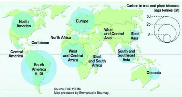
Carbon Stocks over land are distributed mostly between forests and northern latitudes (Figure 1.2), but are mostly found in forests, and more precisely in tropical forests. Indeed, studies suggests that tropical forests play a more important role in absorbing carbon with an absorption rate reaching as much as 1 GtC/year or about 40% of the total land based carbon absorption globally. However, tropical forests are principally located in developing
7 Chapter 1
countries (Amazon basin, Congo Basin, South-East Asia). These countries which are currently undergoing an economic and demographic growth, and therefore moving from forested to non-forested areas are causing a significant impact on the accumulation of greenhouse gases in the atmosphere, as has forest degradation caused by over-exploitation of forests for timber and wood fuel and intense grazing that is reducing forest regeneration. Therefore, during the 16th conference of the parties to the agreement of climate change of
Cancun (2010), the United Nations program for Reducing Emissions from Deforestation and Forest Degradation (UN-REDD) was adopted. This program aims at protecting forests, preserve and increase forest carbon stocks and sustainable forest management. The REDD initiative and its three main supplementary activities are called REDD+. The basic principle of the REDD+ program is that financial compensation be paid by the developed countries to developing countries that manage to reduce their emissions at the national level. The REDD program is based on the fact that when a forest is damaged and destroyed, CO2 is
released into the atmosphere. If we manage to reduce the rate of deforestation (complete disappearance of forests) or degradation (damaged forest due to exploitation), then it is possible to reduce the amount of released CO2. However, in order to calculate the
magnitude of the reduction in CO2 emissions, it is necessary to create a baseline or
reference base against which to compare actual emissions. Therefore it is necessary to be able to quantify the amounts of carbon contained in forests.
Figure 1.2. Forest carbon stock per region. UNEPP, FAO, UNFF, Forest vital graphics, 2009.
Chapter 1 8
1.2.2 Link between carbon and forest biomass
Studies have stated that more than 40% of global vegetation carbon stocks are located in tropical forests ([6]; [12]). However, forest carbon is not limited to trees and is distributed on average as follows: 45% of carbon is found in the soil, 11% in dead biomass or necromass, and 44% in biomass (both above- and below-ground) (FAO, 2000 [13]). Moreover, the above-ground biomass (AGB) is generally the most studied, as it is the most accessible. AGB is a biological material derived from living organisms, and it most often refers to plants. Biomass is carbon based and is composed of a mixture of organic molecules containing hydrogen, oxygen, and small quantities of several other atoms. The proportion of carbon in AGB varies depending on the forest type, wood composition, or the environment. However, it ranges between 0.43 and 0.55 ([14]; [15]; [16]; [17]; [18]).
1.2.3 The importance of quantifying forest biomass
The interest in studying the AGB comes from the fact that the carbon in the AGB is susceptible to be released into the atmosphere by means of deforestation. In addition, land use change in tropical forests is responsible of 15-20% of global greenhouse emissions globally ([19]; [20]). In contrast, if trees are to be planted, this means more carbon sequestration. However, this natural regeneration of the carbon stock will much likely take several decades ([21]), and a plantation is not, by far, a natural forest. Moreover, even with forest degradation or regeneration, tropical forest can still undergo changes that affect AGB levels. For example, under influence of environmental changes, such as the increase of CO2
levels in the atmosphere. This increase of CO2 might increase the photosynthesis of trees
and therefore increase the levels of carbon in trees ([6]; [22]). Other environmental changes are caused by tree mortality, which can increase the necromass, and therefore affect the release of carbon in the atmosphere ([23]).
1.3 Biomass estimation
As seen earlier, AGB measurement is an important task for better understanding of the carbon cycle. However, accurate measurements of biomass require weighing of the trees after cutting them. This method yields high biomass measurement accuracy however it is destructive and restrictive. Therefore it is necessary to find other methods for biomass estimation in a non-destructive manner.
9 Chapter 1
1.3.1 Biomass estimation with optical and radar data
Currently, existing AGB estimation methods from remote sensing data are either limited in the vertical domain (sensor saturation at certain biomass levels using mainly radar and optical data) or in the horizontal domain (limited horizontal coverage using LiDAR data). Methods using radar and optical data for the estimation of AGB are successful in forests with low to medium levels of AGB (e.g. [24]; [25]; [26]; [27]; [28]). Indeed, current techniques based on passive optical sensing have shown limited sensitivity to biomass using medium to high resolution imagery when the biomass reaches intermediate levels (150-200 Mg/ha) (e.g. [27]; [28]). This is due to the optical data inability to detect variation in biomass density after complete closure of the canopy top, which can occur from low or intermediate biomass values (depending on forest characteristics). In contrast, the Fourier Transform Textural Ordination (FOTO) using very-high-resolution optical images have been used for non-saturating estimates of tropical forest biomass estimation. As such, this approach may provide higher sensitivity to biomass high levels (>600 t/ha) (e.g. [29]; [30]; [31]).
The synthetic aperture radar (SAR) systems such as PALSAR/ALOS, JERS-1 and SIR-C, as well as airborne SAR such as SETHI and E-SAR were also used as an alternative for biomass estimation. The radar signal saturation threshold with the biomass increases with the increase of the radar wavelength. Indeed, L-band SAR systems (wavelength about 25 cm) are limited to low and intermediate biomass levels, with maximum values reaching 150 t/ha (e.g. [24]; [25]; [26]; [32]; [33]; [34]). This saturation threshold of the radar signal depends on forest characteristics. According to Imhoff et al. [35]; the saturation levels are closer to 40 t/ha because the saturation thresholds occur before the regression maxima. In boreal forests, saturation levels were observed up to 150 t/ha. Baghdadi et al. [32] observed saturation levels of the ALOS/PALSAR L-band at biomass levels of 50 t/ha when estimating the biomass for Eucalyptus plantations in Brazil. Luckman et al. ([36]; [37]) found a saturation point of 60 t/ha in the Central Amazon basin. Le Toan et al. [26]; Wu et
al. [33]; and Dobson et al. [34] reported L-band signal saturation levels at 100 t/ha in
coniferous forests. In boreal forests, higher saturation levels were observed reaching up to 150 t/ha using PALSAR (Sandberg et al. [25]). However, with higher radar wavelengths (P-band for example, wavelength about 70 cm) the use of SAR sensors may allow the
Chapter 1 10
estimation of biomass at higher biomass levels ([38]). Imhoff et al. [35] examined AGB levels in broadleaf evergreen forests in Hawaii and coniferous forests in North America and Europe and found saturation levels of 100 Mg/ha for the P-band versus 40 Mg/ha for the L-band. Nizalapur et al. [38] found that the sensitivity of radar signal to biomass in a tropical dry deciduous forest increases for approximately 150 t/ha for the L-band to 200 t/ha for the P-band.
Given the limitations of optical (expensive very high resolution images which only cover small areas) and radar (unavailable global coverage for P-band SAR data, signal saturation with lower wavelengths) data for biomass estimation, studies generally use allometric relations for linking the characteristics of a forest (canopy height, diameter at breast height, wood density) to its biomass (e.g. [39]; [40]; [41]).
1.3.2 Biomass estimation using allometric relations
Allometric relationships linking the characteristics of a forest to its biomass were developed by several studies (e.g. [40]; [42]; [39]). The reference model in these studies was developed in the study of Chave et al. [42]. In their study they developed a pantropical biomass estimation model at the individual tree level. This model was based on the formula for calculating the mass of a cylinder using stem diameter (D), canopy height (H), and wood density (ρ).
! = "#. $%&'&. (. ) (1.1) This translates to:
*+,-!/ ="*+,-#/ 0 &. *+,-D/ 1 "2. *+,- &/ 0 *+,-(/ 0 *+,-)/" (1.2) Using the second formula (2), it is possible to predict a tree mass (M) by adding adjustment coefficients:
11 Chapter 1
This model developed by Chave et al. [42] has been shown to produce good biomass estimation results and fits well with data across different tropical forests ([43]).
1.3.3 Plot aggregate allometry for biomass estimation
Asner et al. [40] proposed a plot aggregate allometry model for tropical areas drawn from the Chave et al. [42] model, but they replaced in situ canopy height with top-of-canopy height (TCH), as derived from airborne small-footprint LiDAR measurements, and stem diameter with plot-averaged basal area (BA). BA and wood density were linked with TCH using linear relationships in the form of BA = aTCH and ρ = bTCH + c, producing a model for AGB estimation using only TCH. Results showed a RMSE on AGB estimation of 24.7 Mg/ha for the regional models (model coefficients dependent on region) and 26.4 Mg/ha for the generalized model (generalized model coefficients for all regions). Drake et al. [39] used a power function to link top-of-canopy height estimated from airborne LiDAR to aboveground biomass (AGB = aTCHb). However, this method is considered plot-aggregate allometry rather than true allometry, as it reflects the whole-plot properties of forest structures in aggregate and not the properties of each particular tree. This method had an RMSE of 42.2 Mg/ha when tested in five tropical forests with different vegetation types. Lefsky et al. [44] linked the maximum canopy height (Hmax) estimated from GLAS data to
AGB using the following linear relationship: AGB = a + bH²max. Boudreau et al. [45] linked
the GLAS waveform extent (difference between signal start and signal end), the slope (θ) between signal start and the first Gaussian canopy peak and the terrain index (TI) metric derived from the SRTM-DEM to AGB. Saatchi et al. [46] and Mitchard et al. [24] used Lorey’s height (basal-area-weighted canopy height) instead of the maximum height for AGB estimation. In the different studies, it was found that Lorey’s height is broadly related to canopy height [47]. However, Asner et al. [40] found that Lorey’s height does not explain any variations in AGB, basal area, or wood density that cannot be explained by canopy height.
1.4 Forest canopy height in relation to forest biomass
One of the most important variables in the allometric relations which can be estimated from remote sensing techniques is the canopy height. Several allometries relied on only the canopy height for biomass estimation ([40]; [42]). In addition, studies have shown that the
Chapter 1 12
use of canopy height increases significantly the precision of biomass estimation at tree level (e.g. [14]; [42]). In Chave et al. [42]; the use of tree height reduced relative error on the biomass from 19.5 (model using only DBH and wood density) to 12.8% (model using DBH, wood density and canopy height). In Feldpaush et al. [14]; biomass estimation models which used canopy heights, DBH and wood density showed a 50% decrease in the mean relative error in comparison to the models using only DBH and wood density. Other studies such as Asner et al. [48]; and Mitchard et al. [24] and Lefsky et al. [44] found that canopy height are strongly related to forest biomass. In addition to the importance of forest canopy heights in AGB estimation, knowing forest canopy heights is also interesting in itself for answering ecological questions such as on the determinants of plant and forest structure, forest dynamics, edaphic and climatic stress. Forest canopy heights are very important in forest management decisions; as changes in these heights may have direct effects on microclimatic patterns and processes ([49]). Indeed, the micro climate is modified first by local weather conditions, and then by vegetation, due to forest height which amongst the forest structure, controls the quality and quantity, spatial and temporal distribution of light. It also influences local precipitation and air movements. These factors combined will eventually determine to some extent the humidity in the air, temperature and soil moisture. In addition to having less direct effect on the behavior and distribution of various avian species ([50]; [51]; [52]). Moreover, forest height is important for managing resources such as wildlife, hydrologic response, aesthetics, tree growth and yield ([53]), fire hazard, and susceptibility to insects or disease.
1.4.1 Canopy height estimation using radar and optical data
Studies have used radar data to estimate canopy height using PolInSAR (polarimetric interferometric SAR) (e.g. [54]; [55]; [56]) and tomographic techniques (e.g. [57]; [58]). PolInSAR showed promising results for the estimation of canopy heights. In Neumann et
al. [58]; canopy height estimation using PolInSAR showed an RMSE of 3 m with
maximum canopy heights reaching 40 m when compared to reference canopy height estimates. Garestier et al. [57] estimated canopy heights using P-band PolInSAR data and found an RMSE on the canopy height estimation of 2 m for 2 to 25 m forest heights. However, it was hindered due to several sources of noise (weather changes, atmospheric heterogeneities, and intrinsic phase noise). SAR tomography is an alternative technique for using radar data in canopy height estimation. This technique is an imaging approach, which
13 Chapter 1
generates a fully 3D representation of the imaged scene using coherent combination of a greater number of images ([59]; [60]). Huang et al. [59] used the tomography technique with P-band SAR data for canopy height estimation in a test site in French Guiana. Their results indicated an RMSE on canopy height estimates of 7.7 m. Mercer et al. [60] reported a 10% relative error on tree height estimates in comparison to LiDAR canopy height estimates using SAR tomography with L-band SAR data. SAR tomography is more robust against various noise sources in comparison to PolInSAR at the expense of the necessity to require many more flight lines. The BIOMASS Earth Explorer mission selected by ESA (European Space Agency) in the framework of its living planet program with a P-band spaceborne SAR satellite will provide strong opportunities for the estimation of both canopy heights and biomass from SAR images. Furthermore, many studies used medium and high resolution optical imagery such those available from MODIS, Landsat, Quickbird, IKONOS and others in order to extrapolate airborne or spaceborne LiDAR derived canopy height estimates (e.g. [47]; [61]).
1.4.2 Canopy height estimation using LiDAR data
To this date, canopy height estimation over large areas is best achieved using LiDAR data (either Airborne or Spaceborne). Lidar (Light Detection and Ranging) is an active remote sensing system well suited to measure specific forest information, including but not limited to: canopy heights, basal area, leaf area index, and canopy cover. LiDAR measures object elevation by sending a laser pulse, and measuring the pulse return time, and thus its distance from the LiDAR system and with the help of an onboard GPS, the system determines the objects elevation from the ground. Currently, Airborne LiDAR, is the most accurate remote sensing system to obtain specific site-level data on forest structure. However, wall-to-wall acquisitions of LiDAR data remain very expensive, therefore the use of spaceborne LiDAR systems, which produce free data globally becomes viable. Several studies have estimated canopy height using airborne or spaceborne LiDAR data (e.g. [24]; [44]; [45]; [46]). At regional and global scales, LiDAR data acquired by the Geoscience Laser Altimeter System (GLAS) have been widely used (e.g. [44]; [47]). Using GLAS data, maximum canopy height within each footprint has been successfully estimated with a precision between 2 and 13 m, depending on forest types and characteristics of the study site (e.g. [44]; [62]; [63]; [64]). Lefsky et al. [44] applied linear regressions on waveform metrics and ancillary DEM data for canopy height estimation and obtained site-specific models
Chapter 1 14
with an RMSE between 4.85 and 12.66 m. Hilbert and Schmullius [62] when estimating canopy heights obtained an RMSE of 6.39 m on the canopy height estimation regarding all species and slope classes with a clear negative correlation between accuracy and slope. Lee
et al. [63] applied a slope correction metric to a GLAS estimation model obtained high
correlation between GLAS canopy height estimates and those estimated from a small footprint LiDAR with an RMSE of 2.2 m. Pang et al. [6] estimated the crown-area-weighted mean height with airborne LiDAR measurements using linear regression applied to metrics derived from GLAS waveforms. Their results indicated an RMSE of 3.8 m on the estimation of canopy heights in several coniferous forest sites in western North America.
1.4.3 Spatial extrapolation of LiDAR canopy height estimates
Finally, while LiDAR is very precise with canopy height estimates, it is limited in the horizontal domain (limited spatial coverage for airborne data and limited acquisition density for satellite data). Indeed, airborne LiDAR data are very expensive to acquire for very large areas (€135-175/km2 with 1m point spacing), and while spaceborne LiDAR provides global coverage of waveform data they have a relatively low point density (about 0.51 points/km2 over French Guiana for example). Therefore, it is always necessary to merge LiDAR data (spaceborne or/and airborne) with optical or/and radar data, forest types data, geological data, meteorological data, etc. in order to create forest canopy heights with complete land coverage and a good precision(e.g. [47]; [65]; [66]).
Hudak et al. [66] tested one aspatial (linear regression), two spatial (kriging and co-kriging) and two combined spatial and aspatial methods (kriging and cokriging of regression residuals) for mapping canopy heights using airborne LiDAR canopy height estimates and Landsad Enhanced Thematic Mapper (ETM+) using several sampling strategies (250, 500, 1000 and 2000 m) in a 200 km² study site in western Oregon (USA). Their results showed that the regression model maintained vegetation pattern, however it was more biased towards taller and shorter trees (underestimating taller canopy heights while overestimating shorter ones). Using the regression model, the standard deviation on the canopy height residuals (reference canopy heights – estimated canopy heights) was in the order of 10 m regardless of the sampling strategy. The direct kriging or co-kriging of canopy heights were only slightly more precise than the regression model when predicting canopy heights at
15 Chapter 1
locations lower than 200 m from the reference canopy heights. Moreover, the co-kriging method proved to be slightly more precise than the kriging method. Finally, the method which combined the regression and the kriging and co-kriging of the residuals proved to be the best method for mapping canopy heights. This method conserved the pattern of the canopy heights and improved the precision on the canopy height estimates. The standard deviation on the canopy height estimates varied between 5.5 and 10.9 m for respectively a sampling pattern of 250 and 2000 m.
Lefsky et al. [47] created a global forest canopy height map using regression analysis of canopy heights estimated from the GLAS data and 500 m Moderate Resolution Imaging Spectroradiometer (MODIS) data. The linear regression model which was used to model MODIS data to the GLAS canopy height estimates in order to map forest canopy heights globally showed canopy height estimates with a root mean square error on the estimation of canopy heights of 5.9 m and a coefficient of correlation (R2) of 0.67.
Finally, a more recent study conducted by Simard et al. [65] improved on the work of Lefsky et al. [47] for global canopy height mapping by replacing the linear regression model with the Random Forest technique and using other ancillary data such as the annual mean precipitation, seasonal precipitation, annual mean temperature, seasonal temperature, data from a digital elevation model (DEM) and the percentage tree cover provided from MODIS. Their global canopy height map which was validated against in-situ measurements showed moderate canopy height estimation precision with an RMSE of 6.1 (R² of 0.5) on the estimation of canopy heights.
1.5 Forest types in relation to forest biomass
In addition to the role of forest canopy heights in AGB estimation, forest landscape classification also plays a major role in the methods for estimating AGB. Indeed, many studies have found that AGB estimation models are more relevant when including forest types ([24]; [42]; [67]; [68]; [69]). Zheng et al. [67] found that the coupling of tree metrics acquired from field measurements and various indices derived from Landsat 7 ETM± substantially improved AGB estimates when separating hardwood from pine forests. Chave et al. [42] tested several models for AGB estimation in old growth, dry, moist, wet,
Chapter 1 16
montane and mangrove forests. Their results indicated that one of the most important factors for AGB estimation is forest type. The results also indicated that the best predictive models were forest-type dependent. Ni-Meister et al. [68] developed an AGB estimation model that uses a fusion of LiDAR and optical sensors (to provide the vegetation type) in conifer/softwood and deciduous/hardwood forests. Their results indicated that dependent models provide better AGB estimates in comparison to vegetation-type-independent models. Mitchard et al. [24] found a ±25% uncertainty in the estimation of AGB in Lope National Park (Gabon) using LiDAR data and a vegetation structures map extracted from radar images. Finally, Addo-Fordjour [69] developed AGB estimation models for different species of lianas. Their results indicated that forest type has a significant influence on the allometric relationships used in AGB estimation, which led to forest-type-specific equations.
1.6 Organization of the dissertation
1.6.1 Objectives
The main objective of this thesis was to create new methodologies for the mapping of large forested areas, often inaccessible using remote sensing techniques and especially the one that uses LiDAR. LiDAR remote sensing is an attractive and a complementary technique used with other remote sensing techniques for mapping forest biomass notably through the characterization of the height and the vertical structure of the canopy. However, current missions (satellite or airborne), do not allow the acquisition of LiDAR data with sufficient spatial density measurements for accurate mapping of tree height and subsequently the estimation of biomass at a regional scales. The challenge was then to develop methods for spatial estimation of vegetation height from airborne and satellite LiDAR data and other data sources. The goal is to produce a wall-to-wall canopy height map of French Guiana. From this objective stems different sub-objectives:
- develop a procedure for the estimation of canopy heights from mono-echo airborne LiDAR datasets.
- Evaluate the potential of the LiDAR system ICESat/GLAS to estimate canopy heights in a tropical forest by developing different statistical methods that uses waveforms provided by the ICESat/GLAS system.
17 Chapter 1
- Improve canopy height estimation precision by choosing complementary data issued from different technologies.
- Develop data fusion methodologies using LiDAR canopy height estimates with ancillary data (geological, meteorological phenological ...) in order to propose a forest wall-to-wall canopy height map with good precision and high spatial resolution.
- Analyze the relationship between canopy height estimation precision and the spatial sampling of LiDAR data.
- Evaluate the potential of the ICESat/GLAS data and data from the shuttle radar topography mission (SRTM) for the classification of forest landscape types and forest types.
1.6.2 Dissertation plan
The dissertation contains in total six chapters, including the introduction (chapter 1), chapter 2 which presents the study area and the datasets used, the sub-objectives mentioned in section 1.6.1 are represented in chapters 3, 4, and 5, and, finally the conclusion and perspectives (chapter 6) and the summary of the thesis in French (Chapter 7). In addition, the chapters were written based on scientific articles which were published or submitted at the time of this writing. Each article is introduced later-on in its respective chapter.
Chapter 2 introduces the study area, alongside all the used data in our study. Chapter 3 which is based on a published article in a the peer-reviewed international journal “Remote Sensing” will be dedicated to the introduction of the LiDAR technology (airborne and spaceborne), as well as detailing the methods and procedures used in this thesis in order to estimate canopy heights with either airborne- or spaceborne LiDAR. This chapter starts off with an introduction of the LiDAR datasets used. Next, a detailed description of the methods used in order to estimate forest canopy heights using airborne LiDAR as well as a validation of these estimates is shown. Following that, an introduction of spaceborne LiDAR is presented, as well as the processing of waveforms provided by the ICESat/GLAS and the extraction of the most useful metrics used for canopy height estimation. The remaining of the chapter will be dedicated to the presentation of canopy height estimation methods using ICESat/GLAS with a validation of each method.
Chapter 1 18
Chapter 4 focuses on using the LiDAR based canopy height estimates obtained in chapter 3 as well as ancillary data in order to produce a validated wall-to-wall canopy height map of the entire French Guiana. In addition, the effect of spatial sampling of the LiDAR datasets on the canopy height estimation precision was also studied in this chapter. The contents of this chapter constitute an article that has already been submitted to the remote sensing (MDPI) journal.
Chapter 5 is also based on a published article in the peer-reviewed “International Journal of Applied Earth Observation and Geoinformation”. In this chapter, first, comparisons between elevations extracted from ICESat/GLAS waveforms and elevations from SRTM data were used in order to classify French Guiana’s forest landscape classes. Next, several metrics were extracted from GLAS waveforms in order to classify forest types. Finally, chapter 6 presents the main conclusions and the perspectives of this thesis
2
C
HAPTER
2:
STUDY AREA AND DATASETS
In this study, different datasets were used over our study area for the estimation and mapping of canopy heights. These datasets are comprised of LiDAR data and data from different auxiliary datasets. In order to use the different datasets, filtering, and processing is required. In this chapter, the study is first presented. Next, all the datasets used in this study are presented, as well as any required filtering and processing.
2.1 Study area
French Guiana is situated on the northern coast of the South American continent, bordering the Atlantic Ocean as well as Brazil and Suriname (Figure 2.1)
.
The study site’s area is approximately 83,534 km2, and forest occupies approximately 80,820 km2 or approximately 96.
75% of its total size.
The terrain is mostly low-lying, rising occasionally to small hills and mountains, with an altitude ranging from 0 to 851 m.
In addition, 67.
8% of its slopes are lower than five degrees, 24.
0% are between five and ten degrees and 8.
2% are higher than ten degrees (derived from the SRTM elevations).
Dense tropical forests predominate outside the coastal plain and cover more than four-fifths of the land area.
Chapter 2 20
has an equatorial climate with two main seasons, the dry season, from August to December, and the rainy or wet season, from December to June
.
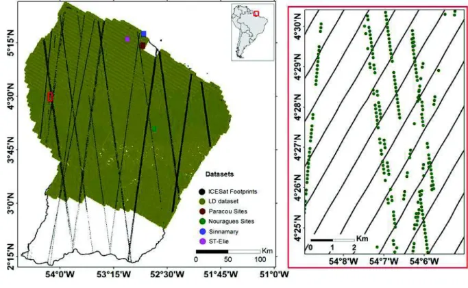
Figure 2.1
.
LiDAR datasets acquired for French Guiana (the right image corresponds to the red rectangle in the left image).
The small rectangles represemtthe location of the HD LiDAR dataset
2.2 Datasets description
2.2.1 Spaceborne LiDAR datasets
LiDAR data were acquired from the GLAS on board the Ice, Cloud, and Land Elevation Satellite (ICESat) between 2003 and 2009
.
The GLAS laser footprints have a nearly circular shape of approximately 80 m in diameter and a footprint spacing of approximately 170 m along their track.
The data were acquired during 18 missions using three on-board lasers with orbit cycles repeating between 57 and 197 days.
Over French Guiana, GLAS data acquisition time coincides with the wet (GLAS acquisition in Feb-March and May-June) and dry (GLAS acquisition in October-November) seasons.
The horizontal geolocation error of the ground footprints is less than 5 m, on average, for all ICESat missions (http://nsidc
.
org/data/icesat/laser_op_periods.
html).
Several studies21 Chapter 2
(e
.
g.
[59]; [70]) have estimated the vertical accuracy of the GLAS to be between 0 and 3.
2 cm over flat surfaces, on average.
From the 15 data products available from the ICESat GLAS, the GLA01 and GLA14 data products were used in this study
.
The GLA01 comprises the full waveform data, and GLA14 comprises the global land surface altimetry data.
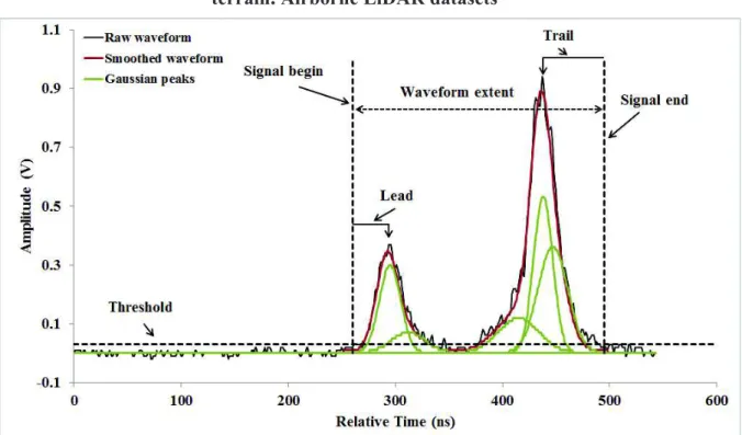
Over flat terrain, the waveforms acquired over vegetated areas are bimodal distributions, with the first peak representing reflections from the canopy top and the last peak representing the ground (Figure 2.2).
To exclude unreliable GLAS data (i.
e.
, data affected by atmospheric conditions, clouds, etc.
), several filters were applied.
(1) Signals with high noise were removed when the signal to noise ratio was higher than 15 (e.g. [70]; [71]; and [63]).
This filter removed 36.
4% of the data.
(2) The GLAS waveforms with delays from either saturation or atmospheric forward scattering were removed (14.
1% of the data).
Only cloudless waveforms were kept using the cloud detection flag (FRir_qaFlag = 15).
This filter removed 32.
4% of the data.
Saturated signals were identified using the GLAS flag (SatNdx > 0)
.
(3) The waveforms with a centroid elevation significantly higher or lower than the corresponding SRTM elevation were removed (|SRTM - GLAS| > 100 m) ([72]).
This filter removed 2% of the data.
(4) The GLAS footprints with SRTM values higher than the GLAS canopy top elevation and lower than the GLAS ground elevation were also removed, which accounted for 33.
4% of the data.
Both the FRir_qaFlag and SatNdx flags were found in the GLA14 product.
From the original database of 101312 footprints, 12238 footprints that satisfied the 4 filters conditions were kept (Figure 2.1).
Finally, the GLAS data referenced to the TOPEX/Poseidon were converted to WGS84 by subtracting 70 cm from the elevation values.
The conversion between the two ellipsoids also depends on latitude; however, as this change is smaller than the horizontal accuracy of the GLAS, it was omitted.
Chapter 2 22
Figure 2
.2
a typical GLAS waveform acquired over a vegetated area on a flat terrain.
Airborne LiDAR datasets2.2.2 Airborne LiDAR datasets
2.2.2.1 Small footprint low density LiDAR dataset
A LiDAR dataset was acquired in 1996 during an airborne geophysical survey that covered 4/5 of French Guiana (northern part, Figure 2.1)
.
Because laser data were acquired for assessing the quality of the survey, and particularly for flight ground clearance, a low sampling frequency was used, and only the first pulse was considered [73]. The data correspond to the elevation of the first obstacle encountered by the laser.
The sampling frequency was 10 Hz with a 905-nm wavelength laser and a footprint size of 35 cm (laser beam divergence of approximately 3 mrad).
The laser measurements are therefore considered point data.
The database contains laser elevations every 7 m on flight lines spaced 500 m apart and oriented at 30°N, intersected by transverse flight lines spaced 5 km apart and oriented at 120°N.
The mean density of this database is approximately 285.
2 points/km2.
Bourgine et al. [74] evaluated the quality of this low-density LiDAR dataset (LD), and the accuracy of the terrain elevation was estimated to be approximately ±2 m.
23 Chapter 2
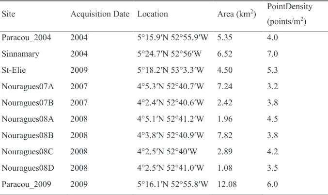
2.2.2.2 Small footprint high density LiDAR dataset
LiDAR datasets with high points density (HD) acquired during several airborne surveys in 2004, 2007, 2008 and 2009 as part of the Guyafor project by a private contractor, Altoa (http://www.altoa.fr/), operating a helicopter-borne LiDAR were used in this study (Table 2.1). These data were previously made available to the ESA Tropisar project. The Biomass project at Jet Propulsion Laboratory (JPL) used this dataset for the evaluation of forest structure estimation from radar data
.
The elevations were recorded using two LiDAR systems: Riegl LMS-Q140i-60 in 2004, 2007 and 2008 and the newer LMS-280i system in 2009.
The elevation data were acquired for several small study sites in French Guiana (Figure 2.1).
The mean acquisition density of the HD datasets is 3.
5 points/m2 (between 3 and 7 points/m2).
The laser wavelength was 905 nm with a mean footprint size of 45 cmfor the first system and 10 cm for the second, and the precision of the elevation was smaller than 0
.
1 m.
Moreover, the HD, unlike the LD, is a last-return laser elevation measurement, as using the last return increased the percentage of ground returns [75].
Table 2.1
.
Description of the HD datasets used in this study.
Site Acquisition Date Location Area (km2) PointDensity (points/m2) Paracou_2004 2004 5°15
.
9ʹN 52°55.
9ʹW 5.
35 4.0 Sinnamary 2004 5°24.
7ʹN 52°56ʹW 6.
52 7.0 St-Elie 2009 5°18.
2ʹN 53°3.
3ʹW 4.
50 5.
3 Nouragues07A 2007 4°5.
3ʹN 52°40.
7ʹW 7.
24 3.
2 Nouragues07B 2007 4°2.
4ʹN 52°40.
6ʹW 2.
42 3.
8 Nouragues08A 2008 4°5.
1ʹN 52°41.
2ʹW 1.
96 4.
5 Nouragues08B 2008 4°3.
8ʹN 52°40.
9ʹW 7.
82 3.
8 Nouragues08C 2008 4°2.
5ʹN 52°40ʹW 2.
89 4.
2 Nouragues08D 2008 4°2.
5ʹN 52°41.
0ʹW 1.
08 3.
5 Paracou_2009 2009 5°16.
1ʹN 52°55.
8ʹW 12.
08 6.0Chapter 2 24
2.2.3 Ancillary datasets
In this study, twelve environmental and geographical variable maps were used. These variables were chosen for their supposed influence on forest characteristics. In addition, these variables are accessible from available free maps (Table 2.2.) The environmental variables will be used later in regression models in order to estimate canopy heights over the entire French Guiana. These variables are: geological map, forest landscape type map, three variable maps computed from SRTM digital elevation model (at 90 m resolution), six variable maps derived from vegetation indices issued from MODIS optical images, and finally one variable map issued from rainfall data
.
Table 2.2
.
Description of the variable maps used for canopy height mapping.
Short name Full name Source Resolution
MIN_EVI Minimum value of EVI time series data
MODIS 250 m
MEAN_EVI Mean value of EVI time series data MAX_EVI Maximum value of EVI time series
data
PC1 1st principal component of EVI time series data
PC2 2
nd principal component of EVI time
series data
PC3 3
rd principal component of EVI time
series data
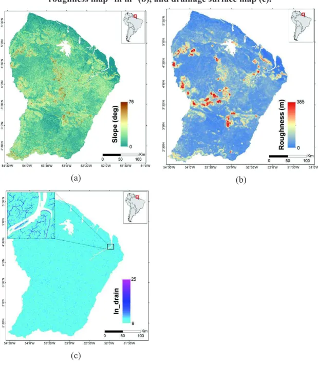
Slope Terrain slope
SRTM 90 m
Roughness Terrain roughness ln_drain Log of drainage surface
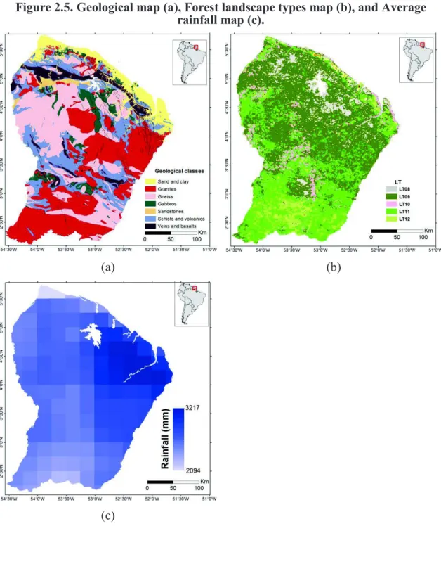
GEOL Geological map Delor et al. [76] Vector
LTs Forest landscape type Gond et al. [77] 1 km (Vector)
Rain mean value of rainfall TRMM 8 km
2.2.3.1 MODerate-resolution Imaging Spectroradiometer (MODIS) data
MODIS sensor mounted on the Terra and Aqua satellites possesses a total of 36 spectral bands of which seven designed specifically for land applications with spatial resolutions that range from 250 m to 1 km