Aggregate Implications of Lumpy Investment: New Evidence and a DSGE Model

Aggregate Implications of Lumpy

Investment: New Evidence and a DSGE Model

The MIT Faculty has made this article openly available.

Please share

how this access benefits you. Your story matters.

Citation

Bachmann, Rüdiger, Ricardo J. Caballero, and Eduardo M. R. A.

Engel. “ Aggregate Implications of Lumpy Investment: New Evidence

and a DSGE Model.” American Economic Journal: Macroeconomics

5, no. 4 (October 2013): 29–67. © 2013 American Economic

Association

As Published

http://dx.doi.org/10.1257/mac.5.4.29

Publisher

American Economic Association

Version

Final published version

Citable link

http://hdl.handle.net/1721.1/95965

Terms of Use

Article is made available in accordance with the publisher's

policy and may be subject to US copyright law. Please refer to the

publisher's site for terms of use.

29

Aggregate Implications of Lumpy Investment:

New Evidence and a DSGE Model

By Rüdiger Bachmann, Ricardo J. Caballero, and Eduardo M. R. A. Engel*

The sensitivity of US aggregate investment to shocks is procyclical. The response upon impact increases by approximately 50 percent from the trough to the peak of the business cycle. This feature of the data follows naturally from a DSGE model with lumpy micro-economic capital adjustment. Beyond explaining this specific time variation, our model and evidence provide a counterexample to the

claim that microeconomic investment lumpiness is inconsequential for macroeconomic analysis. (JEL E13, E22, E32)

U

het-eroscedasticity. Figure 1 depicts a smooth, nonparametric, normalized estimate of the squared residual from fitting an autoregressive process to quarterly aggregate investment rates from 1960 to 2005, as a function of the average recent investment rate. This figure suggests that investment is significantly more responsive to shocks in times of high investment.

In this paper, we show that conditional heteroskedasticity is a robust feature of US aggregate investment rates and that this nonlinearity in the data follows naturally from a DSGE model with lumpy microeconomic investment. The reason for condi-tional heteroscedasticity in the model is that the impulse response function is history dependent, with an initial response that increases by approximately 50 percent from the bottom to the peak of the business cycle. In particular, the longer an expansion, the larger the response of investment to further shocks. Conversely, recovering from investment slumps is hard.

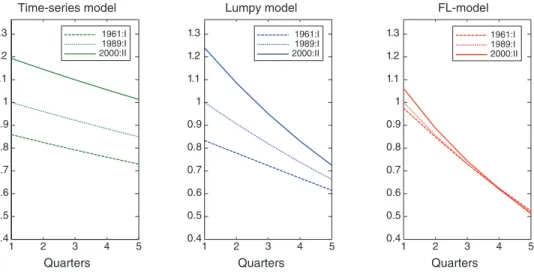
The left and center panels in Figure 2 depict the response over five quarters to a one standard deviation shock taking place at selected points of the US investment cycle, for an ARCH-type time series model and our calibrated lumpy investment DSGE model, respectively.

* Bachmann: RWTH-Aachen University, Templergraben 64, Rm. 513, 52062 Aachen, Germany and CEPR, IFO Institute, and CESifo, (e-mail: ruediger.bachmann@rwth-aachen.de); Caballero: Massachusetts Institute of Technology, Department of Economics, 50 Memorial Drive, Building E52, Room 373A, Cambridge, MA 02142-1347 and National Bureau of Economic Research (e-mail: caball@mit.edu); Engel: University of Chile, Department of Economics, Diagonal Paraguay 257 Piso 14, Santiago, Chile and National Bureau of Economic Research (e-mail: emraengel@gmail.com). We are grateful to Fabian Duarte, David Rappoport, and Jose Tessada for excellent research assistance, and to Olivier Blanchard, William Brainard, Jordi Galí, Pete Klenow, Giuseppe Moscarini, Anthony Smith, Julia Thomas, two anonymous referees, and workshop participants at the American Economic Association annual meeting, University of Bonn, Cornell University, the Econometric Society, Karlsruhe, Mainz, NBER-EFG, New York University, SITE, Stanford University, University of Toulouse, U. de Chile-CEA, and Yale University for helpful com-ments. Financial support from the National Science Foundation (SES 0550134) is gratefully acknowledged.

† _{Go to http://dx.doi.org/10.1257/mac.5.4.29 to visit the article page for additional materials and author}

The periods considered are the trough in 1961, a period of average investment activity in 1989, and the peak in 2000. The differences in the impulse response functions are due to differences in the distribution of productivity levels and capital

Figure 1. Conditional Heteroscedasticity of the Aggregate Investment Rate

notes: This figure depicts a smooth, nonparametric, normalized estimate of the squared resid-ual from fitting an autoregressive process to quarterly aggregate investment rates from 1960 to 2005, as a function of the average recent investment rate. We use a Gaussian kernel and deter-mine the bandwidth via cross-validation. Both the autoregressive process and the average of recent investment rates consider six lags. These choices follow from the results we present in Section I. The dotted lines depict one-standard error bands.

Figure 2. Impulse Response in Different Years–Time Series, Lumpy and Frictionless Models

notes: This figure depicts the response over five quarters to a one standard deviation shock taking place at selected points of the US investment cycle: a trough in 1961, a period of average investment activity in 1989, and a peak in 2000. The figures in the three panels are normalized so that the impulse response in 1989:I (normal investment activity_{) is one upon impact. It does so for an ARCH-type time series model (left panel), our calibrated lumpy} investment DSGE model (center panel), and a frictionless investment model (right panel).

0.023 0.024 0.025 0.026 0.027 0.028 0.029 0.03 0.7 0.8 0.9 1 1.1 1.2 1.3 1.4

Lagged average I/K

Standard deviation of residual

(normalized ) 1 2 3 4 5 0.4 0.5 0.6 0.7 0.8 0.9 1 1.1 1.2 1.3 Time-series model Quarters 1961:I 1989:I 2000:II 1 2 3 4 5 0.4 0.5 0.6 0.7 0.8 0.9 1 1.1 1.2 1.3 Lumpy model Quarters 1961:I 1989:I 2000:II 1 2 3 4 5 0.4 0.5 0.6 0.7 0.8 0.9 1 1.1 1.2 1.3 FL-model Quarters 1961:I 1989:I 2000:II

stocks across productive units. Following a sequence of above average productiv-ity shocks, these units concentrate in a region of the state-space where they are more responsive to any additional shock. The variability of these impulse responses is large and similar in the left and center panels. For example, the immediate response to a shock in the trough in 1961 and to the peak in 2000 differs by roughly 50 percent. The contrast with the right panel of this figure, which depicts the impulse

responses for a model with no microeconomic frictions in investment (essentially,

the standard RBC model_{), is evident. For the latter, the impulse responses vary little} over time.

Beyond explaining the rich nonlinear dynamics of aggregate investment rates, our model provides a counterexample to the claim that microeconomic investment lumpiness is inconsequential for macroeconomic analysis. This is relevant, since

even though Caballero and Engel (1999) found substantial aggregate nonlinearities

in a partial equilibrium model with lumpy capital adjustment, Veracierto _(2002),

Thomas (2002), and Khan and Thomas (2003, 2008) have provided examples in

which general equilibrium undoes the partial equilibrium features.

Why do we reach a different conclusion? Because, implicitly, earlier calibrations imposed that the bulk of investment dynamics was determined by general equilib-rium price responses rather than by adjustment costs. Instead, we focus our calibra-tion effort on gauging the relative importance of these forces, and conclude that

both, adjustment costs and price responses, play a relevant role.

Our calibration begins by noting that the objective in any dynamic macroeco-nomic model is to trace the impact of aggregate shocks on aggregate endogenous variables _{(investment in our context). The typical response of the endogenous} vari-able is attenuated and spread over time by both microeconomic frictions and aggre-gate price responses. We refer to this process as smoothing, and decompose it into

its adjustment cost (AC) and price response (PR) components.

In the context of nonlinear lumpy-adjustment models, AC-smoothing does not merely refer to the existence of microeconomic inaction and lumpiness per se, but to their impact in smoothing the response of aggregates. This is a key distinction in this class of models, as in many instances microeconomic inaction translates into limited aggregate inertia _{(recall the classic Caplin and Spulber 1987 result, where} price-setters follow Ss rules but the aggregate price level behaves as if there were no microeconomic frictions_).

In a nutshell, our key difference with the previous literature is that the latter explored combinations of parameter values that implied microeconomic lumpiness but left almost no role for AC-smoothing, thereby precluding the possibility of fit-ting facts, such as the conditional heteroscedasticity of aggregate investment rates depicted in Figures 1 and 2.

Table 1 illustrates our model’s decomposition into AC- and PR-smoothing. The lower entry shows the volatility of quarterly aggregate investment rates in our model with adjustment costs and price responses. The upper entry reports this sta-tistic when neither smoothing mechanism is present, that is, when adjustment costs are set to zero and prices to their average value in our model with both sources of smoothing. The intermediate entries consider only one source of smoothing at a time, for example, “only AC-smoothing” retains adjustment costs but sets prices

at their average values in the economy that leads to the lower entry. The reduction of the standard deviation of the quarterly aggregate investment rate achieved by AC-smoothing alone amounts to 81.0 percent of the reduction achieved by the combination of both smoothing mechanisms. At the other extreme, the additional smoothing achieved by AC-forces, beyond what PR-smoothing achieves by itself, is 15.4 percent of the total, since PR-smoothing can account for 84.6 percent of total smoothing.

It is clear from Table 1 that both sources of smoothing do not enter additively, so some care is needed when quantifying their relative importance. Averaging the upper and lower bounds mentioned above suggests roughly similar roles for both. By contrast, as discussed in detail in Section III, the contribution of AC-smoothing is typically much smaller in the recent DSGE literature.

Our calibration strategy is designed to capture the role of AC-smoothing as directly as possible. To this effect, we use sectoral data to calibrate the param-eters that control the impact of micro-frictions on aggregates, before general equilibrium price responses have a chance to play a significant smoothing role.

Specifically, we argue that the response of semiaggregated (e.g., three-digit)

investment to corresponding sectoral shocks is less subject to general equilib-rium price responses, and, hence, serves to identify the relative importance of AC-smoothing.

The first row in Table 2 shows the observed volatility of annual sectoral and aggregate investment rates, and their ratio. The second and third rows show these values for our baseline lumpy model and the model with no adjustment costs in investment, respectively. The fourth row reports these statistics for the model

in Khan and Thomas (2008). It is apparent from this table that the frictionless

model fails to match the sectoral data _{(it was never designed to do so). In}

con-trast, by reallocating smoothing from the PR- to the AC-component, the lumpy investment model is able to match both aggregate and sectoral volatility.

Table 1—Contribution of AC and PR Forces to Smoothing of I/K No smoothing

(0.0425) 0 percent

↙ ↘

Only AC smoothing Only PR smoothing

(0.0040) ↓ (0.0036) 81.0 percent 84.6 percent ↘ ↙ AC and PR smoothing (0.0023) 100 percent

notes: This table shows the quarterly volatility of the aggregate investment rate from four models. The upper entry refers to the case when adjustment costs are set to zero and prices to their average value in our baseline lumpy investment model. The intermediate entries consider only one source of smoothing at a time, for example, “only AC-smoothing” retains adjustment costs, but sets prices at their average values in the economy that leads to the lower entry. The lower entry refers to our baseline lumpy investment model with adjustment costs and prices that adjust to clear markets (AC and PR smoothing).

The calibration strategy described above goes a long way toward capturing the heteroscedasticity present in aggregate investment data. It accounts for more than 60 percent of this heteroscedasticity. To match all the heteroscedasticity in aggre-gate investment data, we introduce maintenance and replacement investment as an essential feature of production units, and assume that some within-period main-tenance is necessary to continue operation. Even though there is evidence on the

quantitative relevance of maintenance and replacement investment (e.g., McGrattan

and Schmitz 1999 and Verick, Letterie, and Pfann 2004_{), there is a lack of}

micro-economic studies to help gauge the extent to which these forms of investment are needed to continue operation. We therefore use aggregate statistics, prominent among them a conditional heteroscedasticity measure, to help us identify the main-tenance parameter.

The remainder of the paper is organized as follows. In the next section, we provide additional evidence on conditional heteroscedasticity in aggregate investment data. Section II presents our dynamic general equilibrium model. Section III discusses the calibration method in detail. Section IV presents the main macroeconomic implica-tions of the model. Section V concludes and is followed by several appendices.

I. Conditional Heteroscedasticity

In this section, we present time series evidence for conditional heteroscedasticity in aggregate US investment-to-capital ratios. We also explain why we prefer non-linearity measures based on conditional heteroscedasticity rather than the skewness and kurtosis measures commonly used in the investment literature.

A. Time Series Models

We consider two stationary time series models within the ARCH family to explore whether aggregate investment exhibits the kind of heteroscedasticity predicted by

Ss-type models, namely that investment responds more to a shock during a boom

than during a slump. Both models share the following autoregressive structure:

(1) xt =

∑

j=1

p

ϕ j xt_−j + σ t et ,

Table 2—Volatility and Aggregation

Model 3-digit Aggregate 3-digit/aggregate − ratio

Data 0.0163 0.0098 1.66

This paper 0.0163 0.0098 1.66

Frictionless 0.1839 0.0098 18.77

Khan-Thomas (2008) 0.4401 0.0100 44.01

notes: This table compares annual sectoral and aggregate investment rates, and their ratio, for the data and three models. Sectoral investment data are only available at an annual frequency. The numbers in rows two and three come from the annual analogues of our quarterly baseline models. For details, see Appendices A.B and A.C. The volatility of aggregate investment rates in the Khan and Thomas (2008) entry of this table is taken from table III in their paper. The volatility of sectoral investment rates is based on our calculations.

where xt ≡ i t/ K t denotes the investment to capital ratio, the et are independently and

identically distributed with zero mean and unit variance, and _{σ t} is a simple function of recent values of xt as summarized by the following index:1

(2) _x tk₋₁ ≡ 1 _

k

∑

k xt_−j .

For model 1, we stipulate

(3) σ t = α 1 + η 1 _x tk−1 , while for model 2, we posit

(4) σ t2 = α 2 + η 2 _x tk₋₁ .

It follows from _{(1) that the impulse response of x to e upon impact at time t, denoted} by IR F0, _t , is equal to σ t . Hence, (5) IR F_{0, t =} ⎧ ⎪ ⎨ ⎪ ⎩ α 1 + η 1 _x tk−1 , for model 1;

√

When η 1 = η 2 = 0, the above models simplify to a standard autoregressive time series, with an impulse response that does not vary over time.

The models with lumpy adjustment developed in this paper (and earlier models

such as Caballero and Engel 1999_{) predict positive values for η 1} and _{η 2} . The rea-son is that in these models the cross section of mandated investment concentrates in a region with a steeper likelihood of adjusting when recent investment was high, which implies that investment becomes more responsive to shocks during these times.

B. Estimation and results

Assume observations for x_t are available for t _{= 1, … , T, and denote by p max} and

k max the largest values considered for p and k in (1) and (2), respectively. For all pairs

1 _{This index can be viewed as a parsimonious and robust approximation to the sequence of innovations up to} period t − 1.

(p, k) with p ≤ p max and k ≤ k max, we estimate an AR( p) using OLS, and then use

the residuals from this regression, denoted ϵ t , to estimate α and η via OLS from:2

(6) Model 1: | ε t | =

√

(

)

We choose the optimal values for p and k, denoted by p∗ _{and k} ∗ _{, using the Akaike}

Information Criterion (AIC).

Table 3 presents the estimates obtained for both models; for US private, fixed, nonresidential investment; and for equipment and structures separately. The fre-quency is quarterly, from 1960:I to 2005:IV. We use p _{max = k max = 12.}

The first and second rows report the optimal values for p and k. The following seven rows report statistics related to the magnitude and significance of the

param-eter that captures hparam-eteroscedasticity and time variation in impulse responses, η.

The third row has the point estimate for _{η, and the fourth row has the}

corre-sponding t-statistic, obtained from OLS estimates for (6). The latter may overstate the significance of _{η, since it ignores variations in the first-stage regressions that} determine the autoregressive order, p∗ . For this reason, we use 10,000 bootstrap simulations for the investment rate series, starting from our estimates for e_t in _(1),

to provide an alternative measure of the precision of our estimates for η.3 _The

fifth row presents the p-values we obtain for _{η > 0 via bootstrap simulations. We}

2 _{The first equation is based on}

E [ | ϵ t ||x _ tk−1 ] = √

_

2

_ π ( α 1 + η 1x _ tk−1 ),

while the second equation comes from

E [ ϵ t2 | x _ kt−1 ] = α 2 + η 2 x _ tk−1 .

Also note that we use the same number of observations when estimating all regressions: T − max( p max, k max).

3 _{For each series generated via bootstrap, we estimate the p}

max × k max models and determine the optimal values

for p, k, and, most importantly, η.

Table 3—Evidence of Heteroscedasticity—US Investment to Capital Ratio

Series All Equipment Structures

Model 1 2 1 2 1 2 p∗ _{6 6 7 7 6 6} k ∗ _{6 6 8 8 2 2} η × 1 0 3 _{45.93 0.03731 30.62 0.05380 39.95 0.02581} t − η 3.121 2.496 2.089 1.724 4.097 3.245 p-value(η > 0)-bootstrap 0.0088 0.0236 0.0375 0.0742 0.0033 0.0094 ± log( σ max/ σ min) 0.7367 0.5933 0.5521 0.4395 1.1167 1.1169

± log( σ 95/ σ 5) 0.6118 0.4816 0.4520 0.3547 0.9194 0.8894 ± log( σ 90/ σ 10) 0.5203 0.4082 0.3355 0.2646 0.8003 0.7403 Skewness 0.1574 0.1574 0.3759 0.3759 _{−0.1051 −0.1051} Excess kurtosis _{−0.9803 −0.9803 −0.1401 −0.1401 −0.9864 −0.9864} First-order autocorrelation e_{t −0.0452 −0.0412 −0.0151 −0.0131 −0.0823 −0.0826} Observations 172 172 172 172 172 172

report one-sided p-values since Ss-type models predict η > 0. The next four rows present measures for the range of values taken by the estimated impulse response upon impact; σ max , and σ min denote the largest and smallest heteroscedasticity

esti-mates over the sample considered _{(172 observations), σ p} the p-th percentile. We sign the range estimates by the estimated sign of η. The last row reports the first-order autocorrelation for the estimated innovations _{(the e t} in _{(1)), which are} con-sistent with the independently and identically distributed assumption.

Table 3 shows that nonresidential investment exhibits significant _(both

sta-tistically and economically) heteroscedasticity for both models. This is also the

case for structures, and for equipment under Model 1. The range of heterosce-dasticity values implied by the estimated models is large. For example, the esti-mates for model 2 imply that the ninety-fifth percentile is 61.9 percent larger ( e 0.4816 _{≃ 1.619) than the fifth percentile.}

It also follows from Table 3 that nonlinearities in aggregate investment are much larger (and more significant) for structures than for equipment. This is consistent with a more prominent role for lumpy adjustment in the case of structures.4

Appendix B provides additional evidence supporting our heteroscedasticity find-ing for aggregate investment. We apply the methodology described above to the cyclical component of TFP and find no significant heteroscedasticity. This suggests that the heteroscedastic behavior we find in aggregate investment does not come from the underlying shocks and lends credibility to the explanation we explore in this paper, based on lumpy investment behavior. We also show that there is no signif-icant heteroscedasticity in the cyclical component of GDP, while Berger and Vavra (2012) apply the methodology developed here to durables consumption, which is likely to be subject to similar nonconvex adjustment costs as business investment, and find significant heteroscedasticity.

C. choosing a nonlinearity Measure

In this paper, we introduce a new measure to capture nonlinear relations between shocks and the endogenous aggregate of interest (the investment-to-capital ratio). It is worth comparing this measure with measures that have been used previously in the lumpy investment literature.

Caballero, Engel, and Haltiwanger _{(1995) and Caballero and Engel (1999) used}

skewness and kurtosis of the aggregate investment rate to capture nonlinear

behav-ior, as did Thomas _{(2002) and Khan and Thomas (2003, 2008). This approach is}

justified as follows: If the model’s driving force is Gaussian and the relation between aggregate investment and shocks is linear, the investment rate will also be Gaussian. Finding skewness and kurtosis measures for aggregate investment that differ from those expected under normality can then be interpreted as evidence in favor of a nonlinear relationship.

4 _{Similarly, when comparing lumpy investment models with linear time-series models, Caballero and Engel} (1999) find a much larger reduction in out-of-sample forecast errors for structures than for equipment.

A problem with this approach is that mapping skewness and kurtosis of aggre-gate investment into quantities of interest in macroeconomics is far from obvi-ous. Beyond what threshold do departures from normality in the skewness and kurtosis coefficients become relevant from a macroeconomic perspective? By contrast, the reduced-form time-series models introduced in Section IA estab-lish a direct relation between the nonlinearity measure introduced in this paper

and the impulse response function for aggregate investment (see equation (5)).

Furthermore, a simple function of the parameters of our time-series model mea-sures the time-variation of the impulse response upon impact. This is, we believe, an important advantage when it comes to assessing the macroeconomic relevance of nonlinearities.

A second advantage of the nonlinearity measure we advocate in this paper is that its statistical power is significantly higher than that of the skewness and kurtosis measures. As shown in Appendix B, statistical tests that detect departures from a frictionless RBC-type model using skewness and kurtosis statistics have

consider-ably lower power than tests based on estimates of _{η (or a function thereof) using}

the simple time-series models presented in this section.5 _{It is not surprising that a} statistic especially tailored to capture the specific type of nonlinearity characteristic of Ss models does a better job, as reflected in higher statistical power.

II. The Model

In this section, we describe our model economy. We start with the problem of the production units, followed by a brief description of the households and the defini-tion of equilibrium. We conclude with a sketch of the equilibrium computadefini-tion. We

follow closely Khan and Thomas _{(2008), both in terms of substance and notation.}

Aside from parameter differences, we have three main departures from Khan and Thomas _{(2008). First, production units face persistent sector-specific productivity} shocks, in addition to aggregate and idiosyncratic shocks. Second, production units undertake some within-period maintenance investment, which is necessary to con-tinue operation; some parts and machines that break down need to be replaced. Third, the distribution of aggregate productivity shocks is continuous rather than a Markov discretization, which allows us to back out the aggregate shocks that are fed into the model to produce Figures 2 and 3.

A. Production Units

The economy consists of a large number of sectors, which are each populated by a continuum of production units. Since we do not model entry and exit decisions, the mass of these continua is fixed and normalized to one. There is one commodity in the economy that can be consumed or invested. Each production unit produces this commodity, employing its predetermined capital stock _{(k) and labor (n), according}

5 _{Caballero, Engel, and Haltiwanger (1995) and Caballero and Engel (1999) did not face the statistical power} problem we highlight here because they worked with 20 sectoral investment series instead of one aggregate invest-ment series, as is common in the DSGE literature.

to the following Cobb-Douglas decreasing-returns-to-scale production function (θ > 0, ν > 0, θ + ν < 1):

(7) y_{t = z t ϵ S, t ϵ i, t} k _tθ _{n t}ν _,

where z, _{ϵ S} , and _{ϵ i} denote aggregate, sectoral, and unit-specific _{(idiosyncratic)} pro-ductivity shocks.

We denote the trend growth rate of aggregate productivity by _{(1 − θ)(γ − 1), so}

that y and k grow at rate γ − 1 along the balanced growth path. From now on we

work with k and y _{(and later c ) in efficiency units. The detrended aggregate}

pro-ductivity level, which we also denote by z, evolves according to an AR(1) process

in logs, with persistence parameter _{ρ A} and normal innovations with zero mean and variance σ A2 .

The sectoral and idiosyncratic technology processes follow Markov chains that are approximations to continuous AR(1) processes with Gaussian innovations.6 _The latter have standard deviations _{σ S} and _{σ i} , and autocorrelations _{ρ S} and _{ρ i} , respec-tively. Productivity innovations at different aggregation levels are independent. Also, sectoral productivity shocks are independent across sectors and idiosyncratic productivity shocks are independent across productive units.

Each period a production unit draws from a time invariant distribution, G, its cur-rent cost of capital adjustment, ξ ≥ 0, which is denominated in units of labor. G is a uniform distribution on _[0, __{ξ ], common to all units. Draws are independent across} units and over time, and employment is freely adjustable.

At the beginning of a period, a production unit is characterized by its predetermined capital stock, the sector it belongs to and the corresponding sectoral productivity level, its idiosyncratic productivity, and its capital adjustment cost. Given the aggre-gate state, it decides its employment level, n, production occurs, workers are paid, and investment decisions are made. Upon investment the unit incurs a fixed cost of ωξ, where ω is the current real wage rate. Capital depreciates at a rate δ and a frac-tion of depreciated capital is replaced to continue operafrac-tion. Then the period ends.

We also introduce replacement and maintenance investment as an essential fea-ture of actual production units. This is justified when each productive unit can be viewed as a composite of core and peripheral components, where core components need to be replaced immediately for the unit to continue production. Alternatively, maintaining certain components of a productive unit on a regular basis so that they do not depreciate at all, can be considerably more cost effective than using a stop-go approach to maintenance.7

Note that _{( i} M _{)/(k) ≡ γ − 1 + δ is the investment rate needed to fully}

compen-sate depreciation and trend growth. The degree of necessary maintenance or replace-ment, _{χ, can then be conveniently defined as a fraction of ( i} M_{)/(k). If χ = 0, no}

maintenance investment is needed; if χ = 1, all depreciation and trend growth must be replaced for a production unit to continue operation. We can now summarize the

6 _{We use the discretization in Tauchen (1986), see online Appendix D for details.}

7 _{For instance, maintaining the roof of a structure on a regular basis is likely to dominate over the alternative of} repairing it only when it begins to leak.

evolution of the unit’s capital stock (in efficiency units) between two consecutive periods, from k to k_{′ , after nonmaintenance investment i and maintenance investment}

i M _{take place, as follows:}

Fixed cost paid Future capital k′ Total investment i + i M

i ≠ 0 ωξ any k′ > 0 γk′ − (1 − δ)k

i = 0 0 (1 − χ) _ (1 − δ)

γk k+ χk χ(γ − 1 + δ)k

If i _{= 0 and χ = 0, then k′ = ((1 − δ)k)/(γ), while k′ = k if χ = 100 percent. We} treat χ as a primitive parameter.8

As we will discuss in Section IV, replacement and maintenance investment play an important role in shaping aggregate investment dynamics, since it determines the effective _{(i.e., after maintenance) depreciation rate. This differs from what happens} with linear investment models, where the depreciation rate plays a minor role. We have introduced these determinants of investment in an admittedly stylized manner with a single structural parameter, and leave for future research a more detailed study of these issues.

Given the independently and identically distributed nature of the adjustment costs, it is sufficient to describe differences across production units and their evo-lution by the distribution of units over ( ϵ S , ϵ i , k). We denote this distribution by μ.

Thus, _{(z, μ) constitutes the current aggregate state and μ evolves according to the} law of motion μ′ = Γ(z, μ), which production units take as given.

Next, we describe the dynamic programming problem of each production unit. We take two shortcuts (details can be found in Khan and Thomas 2008, section 2.4). First we state the problem in terms of utils of the representative household _(rather

than physical units), and denote by p = p(z, μ) the marginal utility of

consump-tion. This is the relative intertemporal price faced by a production unit. Second, given the independently and identically distributed nature of the adjustment costs, continuation values can be expressed without explicitly taking into account future adjustment costs.

We simplify notation by writing maintenance investment as

(8) i M _{= (ψ − 1)(1 − δ) k,}

with ψ ∈

[

]

(9) ψ = 1 +

(

)

8 _{We note that our version of maintenance investment differs from what Khan and Thomas (2008) call} “con-strained investment.” Here, maintenance refers to the replacement of parts and machines without which production cannot continue, while in Khan and Thomas (2008) it is an extra margin of adjustment for small investment projects.

Let V1_{( ϵ}

S , ϵ i , k, ξ; z, μ) denote the expected discounted value, in utils, of a unit

that is in idiosyncratic state _{( ϵ i} , _{k, ξ), and is in a sector with sectoral productivity ϵ S} , given the aggregate state (z, μ). Then the expected value prior to the realization of the adjustment cost draw is given by

(10) V 0 _{( ϵ} S , ϵ i , k; z, μ) =

∫

With this notation the dynamic programming problem is given by (11) V 1 _{( ϵ}

S , ϵ i , k, ξ; z, μ) = max _n

{

(

k ′ [−Ac + V A]

)

}

where CF denotes the firm’s f low value; V_i the firm’s continuation value if it chooses inaction and does not adjust; and VA the continuation value, net of adjustment costs Ac, if the firm adjusts its capital stock. That is,

(12A) CF =

[

]

[

]

[

]

where both expectation operators average over next period’s realizations of the aggregate, sectoral, and idiosyncratic shocks, conditional on this period’s values, and we recall that i M _{= (ψ − 1)(1 − δ )k and i = γ k′ − (1 − δ )k − i} M_{. Also, β}

denotes the discount factor from the representative household.

Taking as given intra- and intertemporal prices _{ω(z, μ) and p(z, μ), and the law of} motion μ′ = Γ(z, μ), the production unit chooses optimally labor demand, whether to adjust its capital stock at the end of the period, and the return capital stock, condi-tional on adjustment. This leads to policy functions n = n( ϵ S , ϵ i , k; z, μ) and K = K(

ϵ S , ϵ i , k, ξ; z, μ). Since capital is predetermined, the optimal employment decision is

independent of the current adjustment cost draw. B. Households

We assume a continuum of identical households that have access to a complete set of state-contingent claims. Hence, there is no heterogeneity across households. Moreover, they own shares in the production units and are paid dividends. Following

the argument in Khan and Thomas _{(2008, section 2.4), we focus on the first-order}

conditions of the households that determine the equilibrium wage and the intertem-poral price.

Households have a standard felicity function in consumption and (indivisible) labor:

(13) U ( c, _n h ) _{= log c − A n} h_,

where c denotes consumption and n h _{the fraction of household members that work.}

Households maximize the expected present discounted value of the above felicity function. By definition we have

(14) p (z, μ) ≡ U c ( c, n h ) = 1 _

c (z, μ) ,

and from the intratemporal first-order condition: (15) ω (z, μ) = − _ U n ( c, n h )

p (z, μ) = A _ p (z, μ) .

C. recursive Equilibrium A recursive competitive equilibrium is a set of functions

(

)

that satisfy

(i) Production unit optimality: Taking ω, p, and Γ as given, V 1_{( ϵ}

S , ϵ i , k; z, μ)

solves (10) and the corresponding policy functions are n( ϵ S , ϵ i , k; z, μ) and K_{( ϵ S}, _{ϵ i}, _{k, ξ; z, μ).}

(ii) Household optimality: Taking ω and p as given, the household’s consumption and labor supply satisfy (13) and (14).

(iii) commodity market clearing:

c (z, μ) =

∫

−

∫

∫

ξ

[γ K ( ϵ S , ϵ i , k, ξ; z, μ) − (1 − δ) k] dGdμ.

(iv) Labor market clearing:

n h _{(z, μ) =}

∫

∫

∫

(v) Model consistent dynamics: The evolution of the cross section that charac-terizes the economy, _{μ′ = Γ(z, μ), is induced by K( ϵ S} , _{ϵ i} , _{k, ξ; z, μ) and the} exogenous processes for z, ϵ S , and ϵ i .

Conditions (i), (ii), (iii), and (iv) define an equilibrium given Γ, while step (v) specifies the equilibrium condition for _Γ.

D. Solution

As is well-known, _{(11) is not computable, since μ is infinite dimensional. Hence,}

we follow Krusell and Smith (1997, 1998) and approximate the distribution μ by

its first moment over capital, and its evolution, _{Γ, by a simple log-linear rule. In the} same vein, we approximate the equilibrium pricing function by a log-linear rule: (16A) log _k ′ = a k + b k log

_

k + c k log z,

(16B) log p = a p + b p log

_

k + c p log z,

where _k denotes aggregate capital holdings. Given (15), we do not have to specify an equilibrium rule for the real wage. As usual with this procedure, we posit this form and verify that in equilibrium it yields a good fit to the actual law of motion (see online Appendix D for details).

To implement the computation of sectoral investment rates, we simplify the prob-lem further and impose two additional assumptions: _{(i) ρ S = ρ i = ρ and (ii) enough} sectors, so that sectoral shocks have no aggregate effects. Combining both assump-tions reduces the state space in the production unit’s problem further to a combined technology level ϵ ≡ ϵ S ϵ i . Now, log ϵ follows an AR(1) with first-order

autocorre-lation _{ρ and Gaussian innovations n(0, σ} 2_{), with σ} 2 _{≡ σ}

S

2 _{+ σ}

i

2 _{. Since the sectoral} technology level has no aggregate consequences by assumption, the production unit cannot use it to extract any more information about the future than it has already from the combined technology level. Finally, it is this combined productivity level that is discretized into a 19-state Markov chain. The second assumption allows us to compute the sectoral problem independently of the aggregate general equilibrium problem.9

Combining these assumptions and substituting _k for _{μ into (11) and using (16A)–} (16B), we have that (12A)–(12D) become

(17A) CF =

[

]

[

]

[

]

With the above expressions, (11) becomes a computable dynamic programming problem with policy functions n _{= n(ϵ, k; z,} _k _{) and K = K(ϵ, k, ξ; z,} _k _{). We solve}

this problem via value function iteration on V 0 _{and Gauss-Hermitian numerical} inte-gration over log_{(z) (see online Appendix D for details).}

Several features facilitate the solution of the model. First, as mentioned above, the employment decision is static. In particular, it is independent of the investment decision at the end of the period. Hence, we can use the production unit’s first-order condition to maximize out the optimal employment level:

(18) n _{(ϵ, k; z,} _k _{) =}

(

)

Next, we comment on the computation of the production unit’s decision rules and

value function, given the equilibrium pricing and movement rules _{(16A)–(16B).}

From (17D) it is obvious that neither V A nor the optimal target capital level,

condi-tional on adjustment, depend on current capital holdings. This reduces the number of optimization problems in the value function iteration considerably. Comparing (17D) with (17B) shows that V A(ϵ; z,

_

k _{) ≥ V i(ϵ, k; z,} _k _).10 _{It follows that there exists} an adjustment cost factor that makes a production unit indifferent between adjusting and not adjusting:

(19)  ξ (ϵ, k; z, _k ) = V A (ϵ; z,

_

k ) − V _i (ϵ, k; z, _k )

__ ω (z, _k ) p (z, _k ) ≥ 0.

We define _ξ T_{(ϵ, k; z,} __{k ) ≡ min (} __{ξ ,  ξ (ϵ, k; z,} __{k ) ) . Production units with ξ ≤  ξ} T_{(ϵ, k; z,} __{k )}

will adjust their capital stock. Thus,

k_{′ = K (ϵ, k, ξ; z,} k _) = ⎧ ⎪ ⎨ ⎪ ⎩ k ∗ _{(ϵ; z,} _k ₎ if _{ξ ≤ ξ} T _{(ϵ, k; z,} __{k ),} (20) ψ (1 − δ) k/γ otherwise.

We define mandated investment for a unit with current state (ϵ, z, _k ) and current

capital k as:

Mandated investment _{≡ log γ k} ∗ _{(ϵ; z,} _k _{) − log ψ (1 − δ ) k.}

That is, mandated investment is the investment rate the unit would undertake, after maintaining its capital, if its current adjustment cost draw were equal to zero.

Now we turn to the second step of the computational procedure that takes the value function V 0_{(ϵ, k; z,} __{k ) as given, and prespecifies a randomly drawn sequence of} aggregate technology levels: _{{ z t}. We start from an arbitrary distribution μ 0} , implying a value _k 0 . We then recompute (11), using (17A)–(17D), at every point along the

sequence { z t}, and the implied sequence of aggregate capital levels {

_

k t}, without

imposing the equilibrium pricing rule _(16B):

˜ _V 1 _{(ϵ, k, ξ; z} t , _ k _t ; _{p) = max} n

{

[

]

{

(

[

]

)

}

}

with Vi defined in (12B) and evaluated at

_

k ′ = _k ′( k t). This yields new “policy

functions”:

˜n _{= ˜} n _{(ϵ, k; z t} , _k _t , _p)

˜K _{= ˜} K _{(ϵ, k, ξ; z t} , _k _t , _p).

We then search for a p such that, given these new decision rules and after aggrega-tion, the goods market clears (labor market clearing is trivially satisfied). We then use this p to find the new aggregate capital level.

This procedure generates a time series of { p t} and {

_

k t} endogenously, with

which assumed rules _{(16A)–(16B) can be updated via a simple OLS regression.}

The procedure stops when the updated coefficients ak , bk , ck and ap , bp , cp are

sufficiently close to the previous ones. We show in online Appendix D that the

implied r2 _{of these regressions are high for all model specifications—generally}

well above 0.99—indicating that production units do not make large mistakes

by using the rules (16A)–(16B). This is confirmed by the fact that adding higher

moments of the capital distribution does not increase forecasting performance significantly.

III. Calibration

Our calibration strategy and parameters are standard with two additional features: we combine sectoral and aggregate investment rate volatilities and conditional het-eroskedasticity of the aggregate investment rate in order to infer the relative impor-tance of AC- and PR-smoothing as well as the maintenance parameter.

A. calibration Strategy

The model period is a quarter. The following parameters have standard

val-ues: β = 0.9942, γ = 1.004, ν = 0.64, and ρ _A = 0.95. The depreciation rate δ

matches the average quarterly investment rate in the data, 0.026, which leads to δ = 0.022. The disutility of work parameter, A, is chosen to generate an employ-ment rate of 0.6.

Next we explain our choices for θ and the parameters of the sectoral and

is set to 0.18, in order to capture a revenue elasticity of capital, _ _{1 − ν} θ , equal to 0.5, while keeping the labor share at its 0.64-value.11 _{We determine σ}

S and ρ S by a

stan-dard Solow residual calculation on annual three-digit manufacturing data, taking into account sector-specific trends and time aggregation. This leads to values of 0.0273 for σ _s and 0.8612 for ρ _S .12 _{For computational convenience we set ρ}

i = ρ S ,

and _{σ i} to 0.0472, which leads to an annual standard deviation of the sum of sectoral and idiosyncratic shocks equal to 0.10.13

We turn now to the joint calibration of the two key parameters of the model, the adjustment cost parameter, _ξ , and the maintenance parameter, χ, together with the volatility of aggregate productivity shocks.

With the availability of new and more detailed establishment level data, research-ers have calibrated adjustment costs by matching establishment level moments _(see,

e.g., Khan and Thomas 2008). This is a promising strategy in many instances,

how-ever, there are two sources of concern in the context of this paper’s objectives. First, one must take a stance regarding the number of productive units in the model that correspond to one productive unit in the available micro data. Some authors assume that this correspondence is one-to-one, while others match a large number of model-micro-units to one observed productive unit.14

Second, in state dependent models the frequency of microeconomic adjustment is not sufficient to pin down the object of primary concern, which is the aggre-gate impact of adjustment costs. Parameter changes in other parts of the model can have a substantial effect on this statistic, even in partial equilibrium. For example,

anything that changes the drift of mandated investment (such as the maintenance

investment parameter_{), changes the mapping from microeconomic adjustment costs}

to aggregate dynamics. Caplin and Spulber (1987) provide an extreme example of

this phenomenon, where aggregate behavior is totally unrelated to microeconomic adjustment costs. In the online Appendix E, we present a straightforward extension of this paper’s main model that provides a good fit of observed establishment level moments. This extension adds two micro parameters which, as in the Caplin and Spulber model, have no aggregate _{(or sectoral) consequences, yet can alter} signifi-cantly establishment level moments.

11 _{In a world with constant returns to scale and imperfect competition this amounts to a markup of} approxi-mately 22 percent. The curvature of our production function lies between the values considered by Khan and Thomas (2008) and Gourio and Kashyap (2007). Cooper and Haltiwanger (2006), using LRD manufacturing data, estimate this parameter to be 0.592; Henessy and Whited (2005), using Compustat data, find 0.551.

12 _{See Appendix A, Section C for details and online Appendix C for robustness checks. We note that both this} paper and Cooper and Haltiwanger (2006) use direct evidence on the driving forces to calibrate the parameters for these processes; in our case, evidence at the sectoral level, in the case of Cooper and Haltiwanger (2006), evidence at the plant level. By contrast, Khan and Thomas (2008) treat parameters of the idiosyncratic driving force as a free parameter to match the plant-level investment rate histogram. This may explain why Khan and Thomas (2008) obtain a smaller value for the volatility of idiosyncratic productivity shocks than other studies as well as why their adjustment costs are much smaller than those obtained in other papers (see Table 4). We thank a referee for pointing out this insight.

13 _{In Table 11 in online Appendix C we consider values of 0.075 and 0.15 for the annual total standard deviation,} with no significant changes to our baseline calibration.

14 _{See Cooper and Haltiwanger (2006) and Khan and Thomas (2008) for an example of the former, and Abel} and Eberly (2002) and Bloom (2009), who respectively assume that a continuum and 250 model micro units cor-respond to one observed plant or firm, for examples of the latter.

We believe that ultimately information about investment rates and shock pro-cesses at many levels of aggregation, including the plant or the production unit level, should be brought to bear in order to evaluate richer nonlinear models of invest-ment dynamics. Nevertheless, because of the aforeinvest-mentioned concerns, we follow an approach here where we use three-digit sectoral rather than plant level data to calibrate adjustment costs. More precisely, we choose _{σ A}, __{ξ , and χ jointly to match} three statistics in the data: the volatility of the aggregate US investment rate, the volatility of sectoral US investment rates, and the logarithm of the ratio between the ninety-fifth and the fifth percentile of the estimated values for the conditional het-eroscedasticity of a simple ARCH model _{(see Section IA). We refer to this statistic} as the heteroscedasticity range in what follows.

The novelty in our calibration strategy is that it focuses on matching the rela-tive importance of AC- and PR-smoothing directly. This approach assumes that the sectors we consider are sufficiently disaggregated so that general equilibrium price responses can be ignored while, at the same time, there are enough micro units in them to justify the computational simplifications that can be made with a large num-ber of units. Hence, the choice of the three-digit level.15

Given a set of parameters, the sequence of sectoral investment rates is gener-ated as follows. First, the units’ optimal policies are determined as described in Section IID, working in general equilibrium. Next, starting at the steady state, the economy is subjected to a sequence of sectoral shocks. Since sectoral shocks are assumed to have no aggregate effects and _{ρ i = ρ S} , productive units perceive them as part of their idiosyncratic shock and use their optimal policies with a value of one for the aggregate shock and a value equal to the product of the sectoral and idiosyn-cratic shock—i.e., log(ϵ) = log( ϵ S) + log( ϵ i)—for the idiosyncratic shock.16 The

value of sectoral volatility of annual investment rates we match is 0.0163. To obtain this number we compute the volatilities of the linearly detrended three-digit sectoral investment rates and take a weighted average. As noted in the introduction, this number is one order of magnitude smaller than the one predicted by the frictionless model. To match this annual sectoral volatility in the model simulations, we aggre-gate over time the quarterly investment rates generated by the model.

As shown in Figure 1 and Section IA, the residuals from estimating an autoregres-sive process for aggregate US investment exhibit time-varying heteroscedasticity. We use this information as follows. Given a quarterly series of aggregate investment-to-capital ratios, xt , the moment we match is obtained—both for actual and

model-simulated data—by first regressing the series on its lagged value and then regressing the squared residual from this regression,  e t2 , on xt₋₁ . Denoting by σ 95 and σ 5 the

15 _{Table A3 in Appendix A, Section C provides information on the average number of establishments per} two-digit, three-two-digit, and four-digit sectors, both in absolute terms as well as in relation to the whole US economy. Table 11 in online Appendix C shows that our calibration results do not change significantly if we work with two- or four-digit sectors.

16 _{Online Appendix D.3 describes the details of the sectoral computation. There we also document a robustness} exercise where we relax the assumption that sectoral shocks have no general equilibrium effects, and recompute the optimal policies when micro units consider the distribution of sectoral productivity shocks—summarized by its mean—as an additional state variable. Our main results are essentially unchanged. Finally, it should be noted that our calibration abstracts from relative price effects between sectors that may dampen sectoral investment rate volatilities in response to sectoral shocks.

ninety-fifth and fifth percentile of the fitted values from the latter regression, the heteroscedasticity range is equal to log( σ 95/ σ 5). The target value for the heterosce-dasticity range in the data is 0.3021.17

B. calibration results

The upper bound of the adjustment cost distribution, __{ξ , the maintenance} param-eter, χ, and the volatility of aggregate productivity innovations, σ A, that jointly

match the sectoral and aggregate investment volatilities as well as the conditional heteroscedasticity statistic are _ξ = 8.8, χ = 0.50, and σ A = 0.0080.18 The average

cost actually paid is much lower than the average adjustment cost, __{ξ /2, as shown} in Table 4, since productive units wait for good draws to adjust. The third row shows that, conditional on adjusting, in our calibrated model a production unit pays 3.6 percent of its annual output (column 1) or, equivalently, 5.6 percent of its regular wage bill _{(column 2).}19 _{These costs are at the lower end of previous estimates, as} shown by comparing them with rows 4–6.

The first two rows in Table 4 report the magnitude of adjustment costs for _{χ = 0}

and χ = 0.25. When calibrating these models, we no longer match the

heteroscedas-ticity range in the data, but continue to match both sectoral and aggregate investment

17 _{See Appendix B, Section C for further details on our calibration strategy.}

18 _{Cooper and Haltiwanger (2006) find the mode in the distribution of annual establishment-level investment} rates at 0.04. With an effective annual drift of 0.104, this would suggest a maintenance parameter just below 40 per-cent. Alternatively, McGrattan and Schmitz (1999) show, for Canadian data, that maintenance and repair expendi-tures for equipment and strucexpendi-tures amounts to roughly 30 percent of expendiexpendi-tures on new equipment and strucexpendi-tures. This would suggest just below 25 percent maintenance as a fraction of overall investment. And Verick, Letterie, and Pfann (2004) report that replacement investment in Germany accounts for 66 percent of all investment, which would suggest a value for χ of 0.66. Notice that we do not necessarily need these types of investment to be friction-less, as long as their adjustment costs are much smaller than those for large and lumpy investment projects and are required for the continuing operation of a production unit.

19 _{To compare our findings with the annual adjustment cost estimates in the literature, we report these numbers} for an annual analogue of the quarterly model.

Table 4—The Economic Magnitude of Adjustment Costs—Annual

Adjustment costs/ Adjustment costs/ unit’s output unit’s wage bill

(in percent) (in percent)

Model _{(1) (2)} This paper (χ = 0) 38.9 60.9 This paper (χ = 0.25) 12.7 19.8 This paper (χ = 0.50) 3.6 5.6 Caballero-Engel (1999) 16.5 — Cooper-Haltiwanger (2006) 22.9 — Bloom (2009) 35.4 — Khan-Thomas (2008) 0.5 0.8

Khan-Thomas (2008) “Huge Adj. Costs” 3.7 5.8

notes: This table displays the average adjustment costs paid, conditional on adjustment, as a fraction of output (left column) and as a fraction of the wage bill (right column), for various models. Rows 4–6 are based on table IV in Bloom (2009). For Cooper and Haltiwanger (2006) and Bloom (2009) we report the sum of costs associated with two sources of lumpy adjust-ment: fixed adjustment costs and partial irreversibility. The remaining models only have fixed adjustment costs.

volatilities. For χ = 0.25, the magnitude of adjustment costs lies slightly below the average of those estimated in the literature, for _{χ = 0 they are slightly above the} maximum value, but still within the ballpark.

Table 4 also shows that, ultimately, the main difference between our calibration and Khan and Thomas (2008) is the size of the adjustment cost. As the next to last row indicates, the average adjustment costs paid by firms in the Khan and Thomas (2008) baseline economy are small, compared to the estimates in the literature and our calibration. This is true even for Khan and Thomas’ “huge adjustment costs”

calibration (see Khan and Thomas 2008, section 6), namely a 25 fold increase in

_

ξ . Since the option value of waiting is higher when _ξ is larger, actual adjustment costs are still only one-tenth of what we obtain for the same maintenance parameter, χ = 0. Conversely, for χ = 0 we find that approximately a 400 fold increase in the value of _ξ used by Khan and Thomas (2008) in their benchmark model is needed to jointly match the aggregate and sectoral volatility of investment rates.

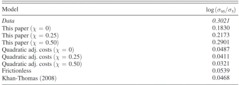
The first two rows of Table 2 and Table 5 show that our model fits both the sectoral and aggregate volatility of investment, as well as the range of conditional heterosce-dasticity in aggregate data. This is not surprising, since our calibration strategy is designed to match these moments. In contrast, the bottom two rows in each of these tables show that neither the frictionless counterpart of our model nor the Khan and

Thomas _{(2008) model match these features.}20

The first row in Table 5 shows the values obtained directly from the data using our ARCH model. The second and third rows show the range of heteroscedasticity

values for versions of our model with values of χ smaller than in the benchmark

case. Even though these ranges now are smaller than those in the data, they continue being significantly larger than those implied by a frictionless model. The model with _{χ = 0 has a heteroscedasticity range three times as large as in the frictionless} model, and it accounts for more than 60 percent of the conditional heteroscedasticity

20 _{As noted earlier, Khan and Thomas (2008) exhibits slightly lower nonlinearity than our calibration of a} fric-tionless model because of differences in the curvature of the revenue function.

Table 5—Heteroscedasticity Range

Model log ( σ 95/ σ 5)

Data 0.3021

This paper (χ = 0) 0.1830

This paper (χ = 0.25) 0.2173

This paper (χ = 0.50) 0.2901

Quadratic adj. costs (χ = 0) 0.0487

Quadratic adj. costs (χ = 0.25) 0.0411

Quadratic adj. costs (χ = 0.50) 0.0321

Frictionless 0.0539

Khan-Thomas (2008) 0.0468

notes: This table displays heteroscedasticity range (log( σ 95/ σ 5)) for the data (row 1) and var-ious model specifications that vary in terms of the maintenance parameter χ and the adjust-ment technology for capital: fixed adjustadjust-ment costs (rows 2– 4), quadratic adjustment costs (rows 5–7), a frictionless model, and the Khan-Thomas (2008) model. The adjustment costs for the models in rows 2–7 have been calibrated to match aggregate and sectoral investment rate volatilities.

found in the data, for the model with _{χ = 0.25 it is four times as large. Both are} much closer to the value in the data than the frictionless model.

Table 5 also shows _{(in rows 5–7) that convex, quadratic adjustment costs do not}

generate significant conditional heteroscedasticity for any level of the maintenance parameter, and are, in fact, close to the frictionless model in this respect. This is not surprising, given that quadratic adjustment cost models lead to partial adjustment in the aggregate and thus to essentially linear aggregate investment rate dynamics.

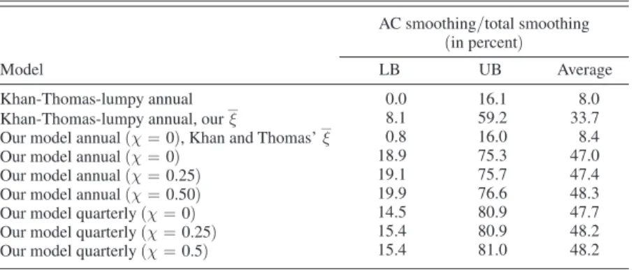
A final way to see the difference between our calibration and Khan and Thomas (2008) is given by a smoothing decomposition, similar to Table 1. Table 6 shows this smoothing decomposition, by reporting upper and lower bounds for the con-tribution of AC-smoothing to total smoothing, for several models, at different fre-quencies. The upper and lower bounds for the contribution of AC-smoothing are calculated as follows:

UB _{= log [σ (NONE)/σ(AC)]/log [σ (NONE)/σ (BOTH)],}

LB _{= 1 − log [σ (NONE)/σ (PR)]/log [σ (NONE)/σ (BOTH)],}

where _{σ denotes the standard deviation of aggregate investment rates, NONE refers}

to the model with fixed prices and with no microeconomic frictions, BOTH to the model with both micro frictions and endogenous price movements, AC to the model that only has microeconomic frictions so that prices are fixed at their average levels of the BOTH specification, and PR to the model with aggregate price responses and no adjustment costs.

The main message can be gathered from the first two rows of this table. By

chang-ing the adjustment cost distribution in Khan and Thomas’ (2008) model for ours,21

its ability to generate substantial AC-smoothing rises significantly. Conversely,

introducing Khan and Thomas (2008) adjustment costs into an annual version of

21 _{Since Khan and Thomas (2008) measure labor in time units (and therefore calibrate to a steady-state value} of 0.3), and we measure labor in employment units, the steady-state value of which is 0.6, and adjustment costs in both cases are measured in labor units, we actually use half of our calibrated adjustment cost parameter. Conversely, when we insert Khan and Thomas (2008) adjustment costs into our model, we double it.

Table 6—Smoothing Decomposition

AC smoothing/total smoothing (in percent)

Model LB UB Average

Khan-Thomas-lumpy annual 0.0 16.1 8.0

Khan-Thomas-lumpy annual, our _ξ 8.1 59.2 33.7 Our model annual (χ = 0), Khan and Thomas’ _ξ 0.8 16.0 8.4

Our model annual (χ = 0) 18.9 75.3 47.0

Our model annual (χ = 0.25) 19.1 75.7 47.4

Our model annual (χ = 0.50) 19.9 76.6 48.3

Our model quarterly (χ = 0) 14.5 80.9 47.7

Our model quarterly (χ = 0.25) 15.4 80.9 48.2

our lumpy model with zero maintenance _{(third row) leads to a similarly small role} of AC-smoothing as in their model. Rows four to nine show the much larger role for AC-smoothing under our calibration strategy, robustly for annual and quarterly calibrations and low and high values of the maintenance parameter.

C. conventional rBc Moments

Before turning to the specific aggregate implications and mechanisms of microeconomic lumpiness that are behind the empirical success of our model, we show that these gains do not come at the cost of sacrificing conventional RBC-moment-matching. Tables 7 and 8 report standard longitudinal second moments for both the lumpy model and its frictionless counterpart. We also include

a model with no idiosyncratic shocks _{(we label it RBC). As with all models, the}

volatility of aggregate productivity shocks is chosen to match the volatility of the aggregate investment rate.22

Overall, the second moments of the lumpy model are reasonable and comparable to those of the frictionless models. While the former exacerbates the inability of

RBC models to match the volatility of employment (we use data from the

establish-ment survey on total nonfarm payroll employestablish-ment from the BLS_{), the lumpy model}

improves significantly when matching the volatility of consumption.23 _{The lumpy}

model also slightly increases the persistence of most aggregate variables, bringing these statistics closer to their values in the data.

22 _{The value of σ}

A required for the frictionless model is σ A = 0.0051, the one for the RBC model is 0.0058.

This shows that lumpy microeconomic adjustment also dampens conventional second moments in our calibration, thereby providing an additional dimension in which nonconvex adjustment costs have macroeconomic implications. Nonetheless, since the focus of this paper is on aggregate nonlinearities (in the relation between the aggregate invest-ment rate and aggregate productivity shocks), we recalibrate σ A for each model so as to match aggregate investment

volatility. Also note that for the lumpy model, the employment statistics are computed from total employment, that is, including workers that work on adjusting the capital stock. We work with all variables in logs and detrend with an HP-filter using a bandwidth of 1,600.

23 _{Consistent with our model, we define aggregate consumption as consumption of nondurables and service} minus housing services. Also, we define output as the sum of this consumption aggregate and aggregate investment.

Table 7—Volatility of Aggregates in Percent

Model Y c i n

Lumpy 1.34 0.83 4.34 0.56

Frictionless 1.11 0.44 5.39 0.73

RBC 1.35 0.45 5.03 0.97

Data 1.36 0.94 4.87 1.27

Table 8—Persistence of Aggregates

Model Y c i n i/K

Lumpy 0.70 0.71 0.70 0.70 0.92

Frictionless 0.69 0.79 0.67 0.67 0.86

RBC 0.70 0.80 0.68 0.68 0.92