HAL Id: hal-01738156
https://hal.inria.fr/hal-01738156
Submitted on 20 Mar 2018HAL is a multi-disciplinary open access
archive for the deposit and dissemination of sci-entific research documents, whether they are pub-lished or not. The documents may come from teaching and research institutions in France or
L’archive ouverte pluridisciplinaire HAL, est destinée au dépôt et à la diffusion de documents scientifiques de niveau recherche, publiés ou non, émanant des établissements d’enseignement et de recherche français ou étrangers, des laboratoires
Cost-effective Bandwidth Provisioning in Microwave
Wireless Networks under Unreliable Channel Conditions
Brigitte Jaumard, Mejdi Kaddour, Alvinice Kodjo, Napoleão Nepomuceno,
David Coudert
To cite this version:
Brigitte Jaumard, Mejdi Kaddour, Alvinice Kodjo, Napoleão Nepomuceno, David Coudert. Cost-effective Bandwidth Provisioning in Microwave Wireless Networks under Unreliable Channel Condi-tions. Pesquisa Operacional, Sociedade Brasileira de Pesquisa Operacional, 2017, 37 (3), pp.525 - 544. �10.1590/0101-7438.2017.037.03.0525�. �hal-01738156�
Cost-effective Bandwidth Provisioning in Microwave Wireless
Networks under Unreliable Channel Conditions
Brigitte Jaumard1, Mejdi Kaddour2, Alvinice Kodjo3, Napole˜ao Nepomuceno4, and
David Coudert3
1Department of Computer Science and Software Engineering, Concordia University, Montreal (QC) H3G
1M8, Canada
2LITIO Laboratory & Department of Computer Science, University of Oran 1, Oran, Algeria 3Universit´e Cˆote d’Azur, Inria, CNRS, I3S, France
4Graduate Program in Applied Informatics, University of Fortaleza, Fortaleza, Brazil
Abstract
Cost-effective planning and dimensioning of backhaul microwave networks under unreliable channel conditions remains a relatively underexplored area in the literature. In particular, band-width assignment requires special attention as the transport capacity of microwave links is prone to variations due to, e.g., weather conditions. In this paper, we formulate an optimization model that determines the minimum cost bandwidth assignment of the links in the network for which traffic requirements can be fulfilled with high probability. This model also aims to increase network reliability by adjusting dynamically traffic routes in response to variations of link ca-pacities induced by channel conditions. Experimental results show that 45% of the bandwidth cost can be saved compared to the case where a bandwidth over-provisioning policy is uniformly applied to all links in the network planning. Comparisons with previous work also show that our solution approach, based on column generation technique, is able to solve much larger instances in significantly shorter computing times (i.e., few minutes for medium-size networks, and up to 2 hours for very large networks, unsolved so far by previous models/algorithms), with a compa-rable level of reliability.
Keywords : microwave networks; mixed-integer linear programming; column generation.
1
Introduction
The advent of broadband mobile services (high definition TV, Voice over IP, Video On Demand) has generated a rapid growth in data traffic, and consequently the need for higher data bandwidth. Due to this growth, ”Backhauling” that means ”getting data to the backbone”, has become a central challenge for network operators. Not only do the operators need to improve customers experience, but they also have to generate sufficient revenues with regard to their capital and operational expenditures. To solve this problem, operators have to install infrastructures that improve their network capacity while using cost-effective technologies. With this regard, microwave technology provides a low-cost alternative to optical fiber when rapid deployment of backhaul high speed data connection is required, in particular for remote or sparsely populated areas [1]. Wireless backhaul market is forecast to grow from $17.85 Billion in 2015 to $33.15 Billion in 2020 [15]. This fast
growth is driven by the vast deployment of 4G networks all over the world. Moreover, high-speed wireless backhauls are foreseen as a critical component to support upcoming 5G networks.
Microwave communication refers to terrestrial point-to-point digital wireless communications, usually employing directional antennas in clear line-of-sight (LOS) and using an electromagnetic wave with a very short wavelength, typically between .039 inches (1 millimeter) and 1 foot (30 centimeters). This makes microwave communications generally free of interference, with nominal capacity near to 500 Mbps nowadays, between two locations that can be several kilometers apart, up to 50 km. However, many questions about how to plan the capacity of wireless microwave networks remain open, especially because of the difficulties in diagnosing channel impairments induced by environmental conditions. Indeed, the provisioning or dimensioning of microwave wireless networks entails a complex design aiming to balance bandwidth-cost efficiency and network reliability, in order to cope with channel fluctuations due to environmental conditions, such as rain or multipath propagation. In particular, adaptive modulation and coding schemes, have shown to dramatically improve link performance [11, 12], but they are more susceptible to errors when using high level QAM (Quadrature Amplitude Modulation) due to channel impairments. In order to maintain an acceptable BER (Bit Error Rate), these techniques involve the variability of link capacity. To deal with this uncertainty, many network operators highly overprovision bandwidth during network planning to avoid traffic bottlenecks and enable smooth capacity degradation under adverse scenarios. This approach, however, incurs avoidable costly investments in addition to spectrum underutilization. As an example, the capital expenditure needed to install one microwave link in France is around e23.000, while the operational cost can reach e22.000 on a year basis [16].
In the present study, we propose an optimization model to tackle the problem of bandwidth provisioning in fixed broadband wireless microwave networks under unreliable channel conditions. In particular, our objective is to determine the minimum cost bandwidth assignment of the links in the network so that a required reliability level of the resulting dimensioning is satisfied, i.e., the selection of bandwidth is made in order to reduce bandwidth costs while ensuring that traffic requirements can be met with high probability. This model relies on the availability, for each mi-crowave link and bandwidth, of a discrete probability distribution of the used modulation schemes. These distributions are derived using typical radio parameters and the widely accepted fading model introduced by Vigants and Barnett [18]. Unlike previous work, we adopt a dynamic routing strategy, where the traffic routes are optimized with respect to current link capacities.
Our solution approach relies on a mixed integer linear programming formulation based on the concept of network configuration, which refers to the network’s state in terms of the used bandwidth and modulation scheme on each transmission link. In order to handle the computational complexity of the problem, the main problem is decomposed, using the column generation technique, into a master subproblem, which determines bandwidth assignment and used configurations, and a pricing subproblem, which tries to improve the current solution by finding new efficient network configurations. Due to its non-linearity and combinatorial nature, we further propose a heuristic procedure to solve the pricing subproblem.
The paper is organized as follows. In Section 2, the recent related studies on dimension-ing microwave networks are discussed. The bandwidth provisioning model, subject to band-width/modulation probability distributions and dynamic routing, is detailed in Section 3. We then describe our solution approach in Section 4. Numerical results are discussed in Section 5 and conclusions are drawn in the last section.
2
Related Work
The inherent variability and unpredictability that characterize microwave transmission due, e.g., to rain precipitation, multipath fading or presence of obstacles, lead to outage events or at least to frequently changing transport capacity. Hence, many works in the literature were concerned with the idea of network reliability. This is typically defined as a numerical parameter, which represents the probability that a subset of nodes in a probabilistic network is connected. However, computing this measure is a classical computationally difficult problem [2, 13], even for the case in which the subset of nodes is restricted to a single source-destination pair, namely, the two-terminal network reliability problem [4].
Dominiac et al. [10] was among the first works to investigate the reliability of fixed broadband wireless networks, but several strong assumptions were behind their model, such as single source-destination flow or uncapacitated network. Furthermore, they considered only the major failures that cause the complete disruption of the communication channel. The authors applied available algorithms for the two-terminal network reliability problem assuming that links fail independently, which is reasonable is this context. Unfortunately, the reported results only corresponds to a small network with 5 nodes and 7 links. Kuo et al. [14] studied the minimum cost problem of connecting a set of base station/gateway sites through a microwave backhaul using different topologies while supporting both time- and space-varying traffic demands. Also, they considered additional constraints of resilience to single link failures. The evaluation results show that meshed wireless backhaul topologies are a cost-effective alternative to trees and rings with respect to spatial and temporal fluctuation of traffic demand and protection against link failures. Nevertheless, the authors assumed fixed link capacities and the derived routing scheme was static, which limits the applicability and performance of their approach.
The problem of determining the minimum cost bandwidth assignment of a network while guar-anteeing a reliability level of the solution was studied in [6, 7]. The authors proposed a chance-constrained programming approach to derive optimal bandwidth assignment and routing of traffic demands while minimizing the network cost and guaranteeing that network flows remain feasible with high probability. Under the assumption that links suffer fading independently, they proposed reformulations to standard MILP models. To the best of our knowledge, the work [8] is the closest to ours. The authors formulated an alternative budget constrained problem for which they present a reliability analysis based on different budgets. Instead of minimizing bandwidth costs, their model aims to maximize the reliability of the network while some budget is not exceeded.
Recently, Coudert et al. [9] designed an algorithm to compute the exact reliability of a backhaul network, given a discrete probability distribution on the possible capacities available at each link. The algorithm computes a conditional probability tree which provides an upper and lower bound on the reliability. Then, it improves these bounds by branching in the tree. The authors provided also an algorithm that exploits properties of the conditional probability tree used to calculate reliability of a given network design subject to a limited budget. A computational study showed that the proposed methods can calculate reliability of large backhaul networks.
In contrast to static routing considered in these previous approaches, we leverage in this paper a dynamic routing scheme to further reduce bandwidth utilization. The general idea is that depending on the available capacity on each link, which may vary over time depending on channel conditions, traffic flows can be rerouted on alternative paths with enough capacity. Hence, over provisioning bandwidth is no longer necessary to make sure that traffic requirements are met in almost all conditions. A necessary assumption here is that network state (i.e., modulation at each link)
typically does not change for a period that is long enough with respect to the time required to propagate rerouting decisions.
3
Problem Statement
3.1 System Model
The topology of a microwave network can be modeled as a digraph G = (V, L), where each node v ∈ V denotes a radio base station and each link ` ∈ L represents a microwave link from u to v, with u, v ∈ V . Let ω+(v) (ω−(v)) denotes the set of outgoing (incoming) links of v. The sets of possible bandwidth values is denoted by B, whereas the set of available modulation schemes is denoted by M . But note that not all the links are eligible to every bandwidth/modulation combination. So, B` ⊆ B and M`⊆ M denote the subsets of bandwidths and modulations, respectively, that can be mapped to a link ` ∈ L. In practice, each m ∈ M may refer to the number of symbols in a M -QAM constellation. Also, the capacity of a link is calculated by the product of the bandwidth value (Hz) and the bandwidth efficiency of the selected modulation scheme (bps/Hz). Each bandwidth b ∈ B installed on some link induces a leasing monetary cost, denoted as costb.
The adaptive nature of the used modulation scheme at some point in time given a bandwidth choice made by the operator is captured through a given discrete probability distribution π, such that
X (b,m)∈B`×M`
π`,bm = 1, ` ∈ L (1)
where π`,bm denotes the probability that modulation m is used together with bandwidth b on link `.
Let’s now introduce a notion that will be used extensively in the rest of the paper: a network configuration c captures the global radio state of the network at some point in time as it refers to the bandwidth selection and the used modulation scheme on each link. Formally, the binary parameter ac`,bm denote whether link ` uses bandwidth b and modulation m within configuration c. Note that only one bandwidth and one modulation value can be associated with each link in a given configuration.
Given some network bandwidth provisioning, we assume also that the used modulations schemes on the different links can be modeled as independent random variables. We believe that this assumption remains reasonable as long as link fades or outages depend more on the characteristics inherent to each link (e.g., distance, topography of the terrain) rather than a common external factor such as the weather. Hence, the probability pc of a network configuration c can be written as: pc=Y `∈L X (b,m)∈B`×M` π`,bmac`,bm c ∈ C (2)
where C represents the set of all possible configurations.
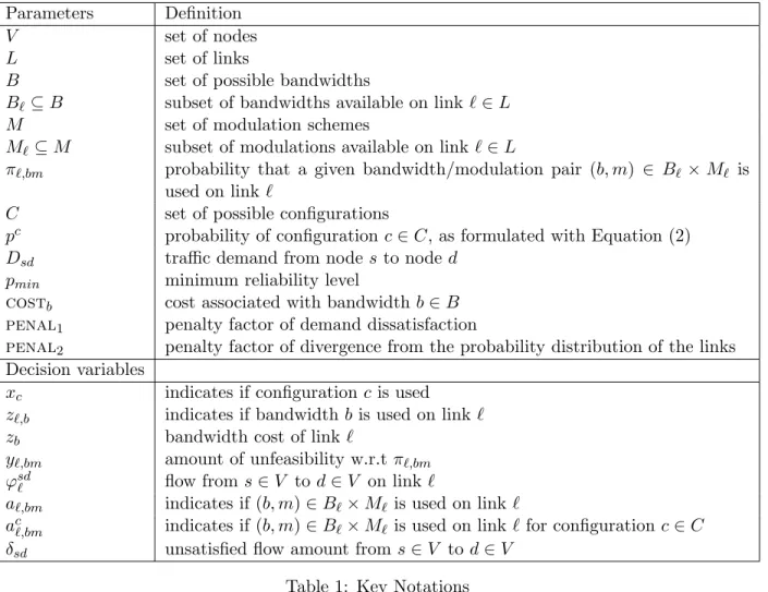
Parameters Definition
V set of nodes
L set of links
B set of possible bandwidths
B`⊆ B subset of bandwidths available on link ` ∈ L
M set of modulation schemes
M` ⊆ M subset of modulations available on link ` ∈ L
π`,bm probability that a given bandwidth/modulation pair (b, m) ∈ B`× M` is used on link `
C set of possible configurations
pc probability of configuration c ∈ C, as formulated with Equation (2) Dsd traffic demand from node s to node d
pmin minimum reliability level
costb cost associated with bandwidth b ∈ B penal1 penalty factor of demand dissatisfaction
penal2 penalty factor of divergence from the probability distribution of the links Decision variables
xc indicates if configuration c is used z`,b indicates if bandwidth b is used on link `
zb bandwidth cost of link `
y`,bm amount of unfeasibility w.r.t π`,bm ϕsd` flow from s ∈ V to d ∈ V on link `
a`,bm indicates if (b, m) ∈ B`× M` is used on link `
ac`,bm indicates if (b, m) ∈ B`× M` is used on link ` for configuration c ∈ C δsd unsatisfied flow amount from s ∈ V to d ∈ V
Table 1: Key Notations
3.2 Optimization Model
Given a set of traffic demands, represented by a matrix D = (Dsd), where Dsd denotes the amount of traffic from node s to node d, both in V , we introduce here an optimization model where the objective is to assign the bandwidth values on the links of L in such a way to minimize the necessary cost to provision the granted demands with a given reliability level pmin, generally close to 1. This probability measure, typically specified by the network operator, constitutes a minimal threshold on the cumulative probability of the configurations retained in the solution. It requires that the determined network provisioning is able to satisfy almost all the traffic demands during at least (pmin∗ 100)% of the time.
Besides, our model encompasses a highly dynamic routing scheme, where the traffic flows can be rerouted on alternative paths from sources to destinations as a result of some shift in the current network configuration. Note however that our problem might not have a solution if one considers only the network configurations that are able to satisfy fully the traffic demands. Hence, the case where some demands are not always correctly provisioned is also considered. In return, this demand dissatisfaction is included in the objective function as a penalty term.
• xc= 1: if network configuration c is included in the solution, 0 otherwise.
• z`,b= 1: if the bandwidth of link ` is b over all the selected configurations, 0 otherwise.
• z`: represents the bandwidth cost of link `.
• y`,bm : amount of unfeasibility with respect to the modulation probability distribution for a given link ` ∈ L and (b, m) ∈ B`× M`.
Note that it may happen that the marginal probability of a bandwidth and modulation choice for some link over the considered configurations is not equal to the initial probability distribution. The role of y`,bm is to increase the reliability level beyond the operator’s initial requirement without increasing the bandwidth cost. In fact, as it will become apparent soon, obtaining an initial feasible solution with a very high pmin can be very difficult and time-consuming, especially if many configurations have very low probabilities. Alternatively, this variable may drive the solution to a sufficiently close reliability level, though the starting point is a much lower pmin.
Our optimization model can be stated as follows:
min X `∈L z`+ penal1 X (s,d)∈D X c∈C δsdc pcxc+ penal2 X `∈L X (b,m)∈B`×M` y`,bm (3) subject to: X c∈C pcxc≥ pmin (4) X c∈C ac`,bmpcxc + y`,bm= z`,bπ`,bm ` ∈ L, (b, m) ∈ B`× M` (5) X b∈B` z`,b= 1 ` ∈ L (6) costbz`,b ≤ z` ` ∈ L, b ∈ B` (7) z`,b ∈ {0, 1} ` ∈ L, b ∈ B` (8) z` ≥ 0 ` ∈ L (9) xc∈ {0, 1} c ∈ C (10) y`,bm∈ [0, 1] ` ∈ L, (b, m) ∈ B`× M`. (11)
Note that in the objective Constraint (3), the terms penal1 and penal2 are positive constants prioritizing the minimization of unsatisfied demand and probability distribution unfeasibility, re-spectively. δsdc is here a constant referring to the amount of unhandled traffic from node s to node d in configuration c. The probability unfeasibility y`,bm for each link is determined in Con-straints (5) according to the selected configurations (xc), the assigned bandwidth b (z`,b) and the used modulation m (ac`,bm).
Constraint (4) ensures that the cumulative probability of the selected configurations is no less than the minimum reliability level pmin. Constraints (6) ensure that a link ` is assigned a unique bandwidth b ∈ B`. Constraints (7) determine the bandwidth cost value for a given link. With constraints (8) and (10), we define explicitly variables z`,b and xc as binary variables. Note that variables z` are not defined as integers in constraints (9) as integrality is implicitly entailed by
the other constraints. Finally, variables y`,bm, corresponding to the probability unfeasibility, are defined in constraints (11) as real numbers in the range [0, 1].
Observe that the number of constraints is in the order of O(|L| × |B| × |M |). This remains quite reasonable as the number of elements in B × M is fairly limited in practice.
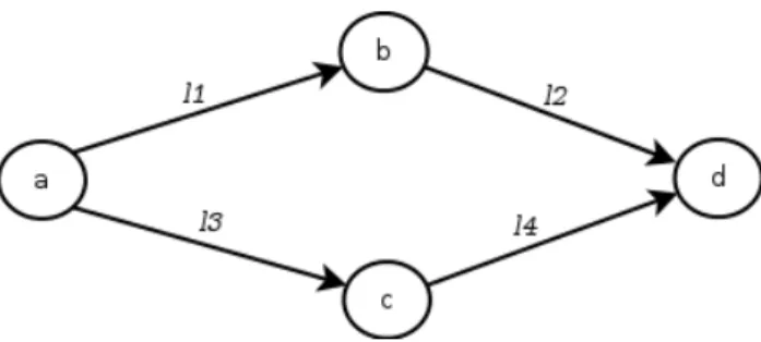
3.3 An Illustrative Example
Figure 1: Examples of a 4-node network
Links π`,b1m1 π`,b1m2 π`,b2m1 π`,b2m2
`1 0.1 0.9 0.2 0.8
`2 0.2 0.8 0.3 0.7
`3 0.1 0.9 0.2 0.8
`4 0.3 0.7 0.4 0.6
Table 2: Modulation discrete probability distributions
Consider the small microwave network shown in Fig. 1 having four links. The following band-width and modulation values are available on each link:
• B = {b1 = 7 MHz, b2 = 14 MHz}
• M = {m1 = QPSK, m2= 16-QAM}
Note that the spectral efficiencies of QPSK and 16-QAM are 2 and 4 bps/Hz, respectively. Hence, the capacity of each link ranges from 14 to 64 Mbps. The total number of network config-uration is 256. Table 3 shows only the 8 most probable configconfig-urations when the bandwidth is set to 7 MHz on each link.
Assume that there is one traffic demand of 40 Mbps from node a to node d, and the required reliability level is 0.85. By assigning just b1 on each link, it can be seen that each network con-figuration from c1 to c5 is able to carry this demand as at most one link is limited to 14 Mbps, while other ones offer 28 Mbps. The cumulative probability of these configurations is 0.8622, which is more than required. Now, if the reliability level is increased to 0.90, more configurations are needed. However, among the remaining configurations, only c7 and c8 can handle a demand traffic greater than 28 Mbps, which is not sufficient. Thus, additional bandwidth is needed which results in higher network cost. Note also that even a reliability level of 0.85 could not be reached if a static routing scheme was used with bandwidth b1 assigned on each link.
L/M c1 c2 c3 c4 c5 c6 c7 c8 `1 m1 0 0 0 0 1 0 0 0 m2 1 1 1 1 0 1 1 1 `2 m1 0 0 1 0 0 1 0 0 m2 1 1 0 1 1 0 1 1 `3 m1 0 0 0 1 0 0 1 1 m2 1 1 1 0 1 1 0 0 `4 m1 0 1 0 0 0 1 1 1 m2 1 0 1 1 1 0 0 0 pc 0.4536 0.1944 0.1134 0.0504 0.0504 0.0486 0.0216 0.0126
Table 3: The 8 most probable network configurations with b1.
4
Solution Approach
4.1 Outline
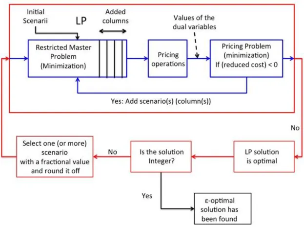
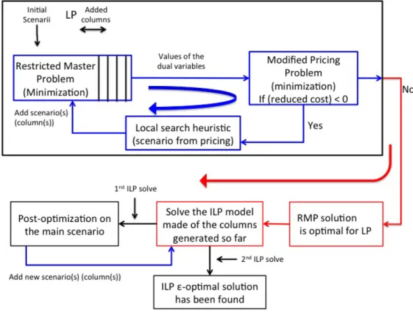
A straightforward solution approach to our model (3)-(11) is to include all the possible network configurations in C: this is clearly intractable even with moderate-size network instances. Alter-natively, we describe hereafter a solution process based on the Column Generation technique (CG) which splits the original problem into two subproblems: the Restricted Master Problem (RMP) and the Pricing Problem. The RMP is a linear-relaxed version of the original problem where only a limited subset of configurations are considered, while the pricing is another problem created to generate only the variables (configurations) which have the potential to improve the objective function, i.e., to find variables with negative reduced costs. As depicted in Fig. 2, the process alternates between these two problems until the following optimality condition is satisfied: no more configurations with a negative reduced cost can be derived. At this point, if all the variables of the RMP have integer values, the process is done and the solution is optimal. Otherwise, the RMP is solved again by enforcing integrality constraints on the current variables (or columns) xc and also z`,b. This latter solution can be thought as an upper-bound solution of the original problem, not necessarily optimal. Nevertheless, as shown by our experimentations, the gap with the lower-bound LP-relaxed solution is generally very narrow.
The objective of the pricing problem consists in minimizing the reduced cost of variables xc. The reader who is not familiar with linear programming is refereed to the seminal books of [3, 5] for its computation. Indeed, in linear programming, the reduced cost is the amount by which an objective function coefficient would have to decrease before it would be possible for a non basic variable to assume a positive value in the optimal solution. It is therefore written as follows:
costc= penal1 X (s,d)∈D X c∈C δsdc pc | {z }
initial cost of variable xc
− columnc· u, (12)
where columnc is the column vector associated with variable xc and u is the dual vector of the linear program associated with (3)-(11) (i.e., where the domain of the binary variables has been changed to [0,1]).
Figure 2: The column generation decomposition technique.
We now omit the c index in order to alleviate the notations. Based on (3)-(5), this leads to:
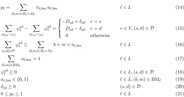
cost = Y `∈L p` penal1 X (s,d)∈D δsd− u(4)− X `∈L X (b,m)∈B`×M` u(5)`,bma`,bm (13)
where u(4) (≥ 0) and u(5)`,bm (≶ 0) are dual values corresponding to Constraints (4) and (5), respec-tively. p` represents the probability that the link ` uses the affected bandwidth/modulation in the configuration under construction. Here, each variable δsdrepresents the unsatisfied flow amount for the demand (s, d) ∈ D, and each binary variable a`,bm indicates if the bandwidth b and modulation m are used on link `. The set of constraints of the pricing problem can be written as follows:
p`= X (b,m)∈B`×M` π`,bma`,bm ` ∈ L (14) X `∈ω−(v) ϕsd` − X `∈ω+(v) ϕsd` = −Dsd+ δsd v = s Dsd− δsd v = d 0 otherwise v ∈ V, (s, d) ∈ D (15) X (s,d)∈D ϕsd` ≤ X (b,m)∈B`×M` b × m × a`,bm ` ∈ L (16) X (b,m)∈BM` a`,bm = 1 ` ∈ L (17) ϕsd` ≥ 0 ` ∈ L, (s, d) ∈ D (18) a`,bm ∈ {0, 1} ` ∈ L, (b, m) ∈ BM` (19) δsd≥ 0 (s, d) ∈ D (20) 0 ≤ p`≤ 1 ` ∈ L (21)
where the variable ϕsd` represents the amount of flow transported from node s to node d. Con-straints (15) enforce the flow conservation at each node, while conCon-straints (16) limit the flow carried on each link to the transport capacity as defined by the selected bandwidth/modulation pair. Con-straints (17) ensure that a unique pair bandwidth/modulation is selected for link `.
Unfortunately, finding exact solutions to this problem is rather challenging as the objective function includes a highly non convex term (product of p` variables). In the sequel, a heuristic approach is proposed with the aim to find high-quality solutions in a timely manner.
4.2 Modified Column Generation (MCG) heuristic
The main difficulty to solve the pricing problem stems from the presence of a non convex term in the objective. However, it can be easily seen that this term (Q
`∈LP`) does not affect the sign of the objective value, as it is the product of positive quantities. Hence, if the reduced cost of some configuration is negative, it will still be the case if this term is omitted from the objective. So, the modified pricing problem becomes a regular MILP that can be solved with off-the-shelf solvers. Obviously, this trick does not apply without some loss in the solution quality. In fact, nothing prevents now from getting configurations with very low probabilities. As a result, compared to exact pricing solutions, much more iterations between the RMP and the pricing may be required to build the final solution.
To mitigate this effect, we consider only the configurations that satisfy the totality of the traffic requirements (i.e., δsd = 0, ∀(s, d) ∈ D). Furthermore, the speed of the resolution process is increased by trying to add several configurations in one iteration. To this end, we define a local search heuristic which looks for other configurations with negative reduced cost starting from the one returned by the modified pricing. Such configurations, called neighbor configurations, are found by modifying only the modulation of a number of randomly selected links while ensuring the satisfaction of the traffic requirements. Algorithm 1 describes the process.
Fig. 3 represents the overall resolution process, where a post-optimization procedure is applied after the final ILP resolution of the RMP. This procedure works as follows: it first selects the
Figure 3: Overall resolution process with the MCG heuristic
configuration c that has the highest probability among those that were selected by the ILP resolution of the RMP. Note that the bandwidth assignment is already done at this stage. Then, additional configurations are derived by modifying the modulation of some randomly chosen links of c. This modified pricing problem is used to verify the existence of a routing solution for these configurations. If so, they will be added to the solution. This contributes to increase the network reliability without increasing the bandwidth cost.
4.3 Initial Solution of the RMP
A certain number of network configurations must be given to the RMP model in order to obtain the first feasible solution of the problem. In particular, as stated in (4), the cumulative probability of these configurations must be no less than pmin. Finding such configurations can be tedious for large network instances and high values of pmin.
We tackle this issue by solving a modified version of the RMP, where the objective function is rewritten as follows: max X c∈C pcxc− penal1 X (s,d)∈D X c∈C δsdc pcxc (22)
Algorithm 1: Local Search Heuristic
Input : a configuration c with negative reduced cost (redcost(c) < 0) Output: a set of configurations Nc
iter ← 1; ¯c ← c; Nc← ∅ while iter ≤ #M axIter do
I(¯c) ← a set of ∆ neighbor configurations of ¯c foreach c0 ∈ I(¯c) do if redcost(¯c) < 0 then Nc← Nc∪ {¯c} end end ¯ c ← arg min c0∈I(¯c) redcost(c0) iter ← iter + 1 end return Nc
able to satisfy all the traffic demands, so that constraint (4) holds. Naturally, this latter constraint is dropped from the formulation.
The objective function of the corresponding pricing problem needs to be modified to reflect the new reduced cost. It can be written as:
max Y `∈L p` 1 − penal1 X (s,d)∈D δsd − X `∈L X (b,m)∈B`×M` u(5)`,bma`,bm (23)
while the set of constraints is not modified.
Again, we work around the non-linearity in the objective using the heuristic approach described in the previous section. As the objective now is a maximization, a new configuration will be added to the initial RMP if its reduced cost is strictly positive. Finally, the process switches to the main RMP model as soon as a feasible solution is obtained.
5
Numerical Results
In this section, we describe and discuss several numerical experiments that have been conducted to evaluate the computational performance of our approach and the quality of the obtained provi-sioning solutions. The experimental problem data consists in a set of real-world network topologies proposed by SNDlib [17] with the traffic demands rescaled as in [8]: Atlanta (15 nodes, 44 links), Polska (12 nodes, 36 links), France (25 nodes, 90 links) and Germany50 (50 nodes, 176 links) (see Fig. 4).
Each link can be assigned a bandwidth of 7 MHz, 14 MHz or 28 MHz. Available modulation and coding schemes for these bandwidths, their bandwidth efficiency and required SNR levels are presented in Table 4. In sum, 18 bandwidth/modulation pairs are available on each link. Note that the network instances as well as the radio parameters are identical to those used in [8]. According to the Vigants-Barnett radio fading model [18], we observe that most of the time, each link will be transmitting at the highest modulation.
Figure 4: Three used topologies (from left to right, Atlanta, France, Germany50) [17]
Besides, the monetary cost of 1 MHz of bandwidth is set to $1000. Note also that the overall resolution time is limited to two hours. Other relevant parameters are: pmin = 0.9; penal1 = 40, 000; penal2 = 50. Theses values are chosen with the aim to obtain solutions that are more focused on satisfying almost fully traffic demands rather than achieving a very high reliability level.
MCS Bandwidth efficiency (bps/hz) Required SNR (dB)
m1: 16-QAM coded 3.6 21.02 m2: 16-QAM uncoded 4.0 21.02 m3: 64-QAM coded 5.4 27.45 m4: 64-QAM uncoded 6.0 27.45 m5: 256-QAM coded 7.2 33.78 m6: 256-QAM uncoded 8.0 33.78
Table 4: Modulation schemes and bandwidth efficiency
5.1 Resolution process
First, let us point out that the high variability of the probability distributions described above and the independence between link probabilities produce a tremendous number of possible tions with very low probability value. In order to prevent generating such meaningless configura-tions, e.g., with probability of the order of 10−75, the following restriction is added to the pricing problem: p` ≥ 0.1 for ` ∈ L.
Topology Polska Atlanta France Germany50
# Total conf. 606 635 629 454
# Used conf. 78 16 102 17
Table 5: Column Generation Process
For each considered topology, Table 5 shows that the total number of configurations generated by our solution process, using the MCG heuristic, represents only a tiny fraction of the overall number of possible configurations, i.e., Q
`∈L|B` × M`|. That means that our solution process focuses primarily on the most significant configurations in terms of probability and demand satisfaction.
Also, we can observe that the best solutions in terms of cost will retain only a limited number of configurations while reaching the desired reliability level. Note that most generated configurations satisfy all traffic demands, i.e., δsd = 0 for all (s, d) ∈ D.
5.2 Solution quality
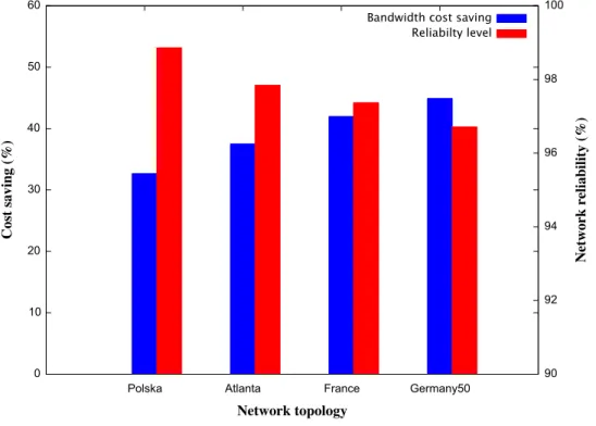
We evaluate here the quality of the solutions obtained by our optimization model using the MCG heuristic. Fig. 5 shows, for each network topology, the cost saving that can be achieved by the network operator compared to the worst case where the highest cost bandwidth is provisioned on every link. We observe a significant cost saving ranging from 33% to 45%, while reaching a high reliability level. This gain is more noticeable with larger networks, but it goes with some decrease of the service reliability. This is due in part to the additional constraint on p`(p` ≥ 0.1), but mainly to the fact that it is much harder to achieve the same reliability when the network is constituted by more links as configuration probabilities tend to zero. For instance with Germany50, for a configuration c where each link ` ∈ E is such that p` = 0.9, we have pc= 0.9176' 10−8.
Figure 5: Cost saving vs. the worst case
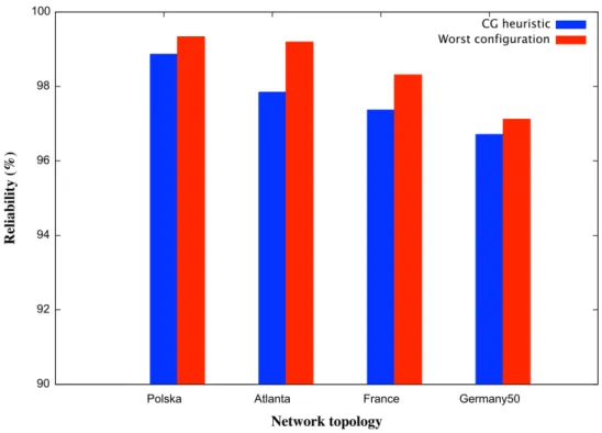
Another way to assess the performance of our method is to measure the reliability gaps between our solutions and the worst case provisioning. As depicted in Fig. 6, one can see that the reliability level is only slightly compromised while the bandwidth cost is significantly reduced.
5.3 Comparison with some results from [8]
We compare here our results with those reported by Claßen et al. [8]. First, let us note that the problem addressed in [8] has a different objective: reliability maximization for a fixed budget
Figure 6: Reliability vs. the worst case
Polska Atlanta France Germany50
CG-MCG 7 32 131∗ 148∗
Budget-constrained [8] 21 120 nf –
∗: CG process is stopped after 2 hours.
nf: no feasible solution was reported, – : not considered.
Table 6: Resolution time (minutes)
or cost. Furthermore, the derived routing scheme is static (i.e., does not depend on the current radio conditions). The problem is solved multiple times for decreasing budgets until no solution can be found. While this approach allows finding a good compromise between cost and reliability, its drawback lies in its very long required computational time in order to find the minimum cost solution.
In case of budget-constrained model, the reported solutions, which were obtained using the fastest method (i.e., adding cutset inequalities), achieve 36%, 39% and 40% of cost savings for Polska, Atlanta and France networks, respectively (Germany50 has not been considered in [8]). Results depicted in Fig. 7 show that, using the methods presented in this paper, we obtained a lower cost for Atlanta and France. Whereas, Fig. 8 shows that achieved reliability are inferior by no more than 1% for Polska and Atlanta, while our approach performs better on the France instance as no solution has been found using the budget-constrained model with the same cost.
In sum, budget-constrained model provides better solutions for small network instances while our approach based on column generation scales much better. We even believe that obtaining feasi-ble solutions with the budget-constrained approach in a reasonafeasi-ble amount of time is very unlikely
Figure 7: Cost comparison with [8]
for large instances, such as Germany50. Table 6 summarizes a comparison of the computation times required in both cases with a similar cost. Not only our approach is the fastest one, but it also provides good results for large instances in a relatively limited amount of time.
6
Conclusion
In this paper, we have introduced an optimization model for the minimal-cost bandwidth provi-sioning in microwave networks under unreliable channel conditions. The model formulated initially as mixed-integer linear program was solve using the a column generation-based decomposition ap-proach to separate the bandwidth assignment from traffic routing that depends on the current network’s state. Each valid solution must conform to a minimum operator-specified reliability level in presence of fluctuations in the transport capacity of links. As our model raises a number of difficulties due the non-convexity of the pricing subproblem, a computationally-efficient heuristic has been proposed. Numerical results confirm the substantial operational costs gains that can be made while achieving a satisfactory reliability level. Also, the potential of our approach on large scale instances has been assessed. In particular, our approaches was able to solve instances that were not reachable by previous methods.
As future work, we plan to improve the heuristic used to solve the pricing problem in order to increase the reliability of the solutions, and eventually find solutions with smaller cost. We would also like to propose a fixed budget formulation in order to build the Pareto front of the solution space. Moreover, correlation between the links fades due to environmental (weather) conditions
Figure 8: Reliability comparison with [8]
will a subject of a thorough investigation.
References
[1] H. Anderson. Fixed Broadband Wireless System Design. John Wiley & Sons, first edition, 2003.
[2] M. O. Ball. Computational complexity of network reliability analysis: An overview. IEEE Transactions on Reliability, 35(3):230–239, 1986.
[3] M. Bazaraa, J. Jarvis, and H. Sherali. Linear Programming and Network Flows. Wiley, New York, 1977.
[4] T. B. Brecht and C. J. Colbourn. Lower bounds on two-terminal network reliability. Discrete Applied Mathematics, 21(3):185 – 198, 1988.
[5] V. Chvatal. Linear Programming. Freeman, 1983.
[6] G. Claßen, D. Coudert, A. M. C. A. Koster, and N. Nepomuceno. Bandwidth assignment for reliable fixed broadband wireless networks. In 12th IEEE International Symposium on a World of Wireless Mobile and Multimedia Networks (WoWMoM 2011), pages 1–6, 2011.
[7] G. Claßen, D. Coudert, A. M. C. A. Koster, and N. Nepomuceno. A chance-constrained model & cutting planes for fixed broadband wireless networks. In 5th International Network Optimization Conference (INOC 2011), volume 6701 of LNCS, pages 37–42. Springer, 2011.
[8] G. Claßen, D. Coudert, A. M. C. A. Koster, and N. Nepomuceno. Chance-Constrained Opti-mization of Reliable Fixed Broadband Wireless Networks. INFORMS Journal on Computing, 26(4):893–909, 2014.
[9] D. Coudert, J. Luedtke, E. Moreno, and K. Priftis. Computing and maximizing the exact reliability of wireless backhaul networks. In International Network Optimization Conference, Lisbon, Portugal, Feb. 2017.
[10] S. Dominiak, N. Bayer, J. Habermann, V. Rakocevic, and B. Xu. Reliability analysis of IEEE 802.16 mesh networks. In 2nd IEEE/IFIP International Workshop on Broadband Convergence Networks, BcN 2007, pages 1–12, 2007.
[11] A. Goldsmith and S.-G. Chua. Variable-rate variable-power MQAM for fading channels. IEEE Trans. Commun., 45:1218–1230, 1997.
[12] A. Goldsmith and S.-G. Chua. Adaptive coded modulation for fading channels. IEEE Trans. Commun., 46(5):595–602, 1998.
[13] P. Hansen, B. Jaumard, and G.-B. D. Nguetse. Best second order bounds for two-terminal network reliability with dependent edge failures. Discrete Applied Mathematics, 96(97):375– 393, 1999.
[14] F. C. Kuo, F. A. Zdarsky, J. Lessmann, and S. Schmid. Cost-efficient wireless mobile backhaul topologies: An analytical study. In Global Telecommunications Conference (GLOBECOM 2010), 2010 IEEE, pages 1–5, Dec 2010.
[15] marketsandmarkets.com. Mobile and wireless backhaul market by equipment (microwave, millimeter wave, sub 6 ghz, test and measurement), by services (network, system integration, professional) - worldwide market forecasts and analysis to 2015 - 2020, December 2015.
[16] N. Nepomuceno. Network optimization for wireless microwave backhaul. PhD thesis, Ecole doctorale STIC, Universit´e Nice-Sophia Antipolis, Dec. 2010.
[17] S. Orlowski, R. Wess¨aly, M. Pi´oro, and A. Tomaszewski. Sndlib 1.0 - survivable network design library. Networks, 55(3):276–286, 2010.
![Figure 4: Three used topologies (from left to right, Atlanta, France, Germany50) [17]](https://thumb-eu.123doks.com/thumbv2/123doknet/13647323.428006/14.918.158.764.113.327/figure-used-topologies-left-right-atlanta-france-germany.webp)
![Figure 7: Cost comparison with [8]](https://thumb-eu.123doks.com/thumbv2/123doknet/13647323.428006/17.918.184.720.110.528/figure-cost-comparison-with.webp)
![Figure 8: Reliability comparison with [8]](https://thumb-eu.123doks.com/thumbv2/123doknet/13647323.428006/18.918.177.719.116.525/figure-reliability-comparison-with.webp)
