Bulk properties and atmospheric structure of Pluto and Charon

BULK PROPERTIES AND ATMOSPHERIC STRUCTURE

OF

PLUTO AND CHARON

by

Leslie Ann Young

A. B., Physics, Harvard College (1987)

Submitted in Partial Fulfillment of the Requirements for the Degree of

DOCTOR OF PHILOSOPHY in

EARTH, ATMOSPHERIC, AND PLANETARY SCIENCES at the

MASSACHUSETTS INSTITUTE OF TECHNOLOGY

June 1994, L

--© 1994 Massachusetts Institute of Technology, All Rights Reserved

Signature of Author ... ... ... ... ..

Department of Earth,-Atmospheric, and tary Sciences June 21, 1994

Certified

by ...

...

Professor James L. Elliot Thesis Supervisor Department of Earth, Atmospheric, and Planetary Sciences

Accepted

by ...

.

.-

'I...

Professor Thomas Jordan Chairman, Department Graduate Committee

ARCHIVES

MASSACHSE,7T INSTITUTE OF "rc'Hl*4 nif Iy

ABSTRACT

We present three observational programs to investigate Pluto's atmospheric structure and the bulk properties of Pluto and Charon: (i) astrometry of the motions of Pluto and

Charon around the system barycenter to determine their individual masses; (ii) analysis of a stellar occultation to find temperatures and pressures in Pluto's middle atmosphere; and (iii)

spectroscopy of gaseous CH4to find its abundance in Pluto's atmosphere. The astrometric

observations, taken from 1992 Feb. 26 to 1992 Mar. 2 at the University of Hawaii 2.2-m telescope on Mauna Kea, indicate Pluto and Charon masses of (12.38 ± 0.12) x 1024 g and (1.94, 0.04) x 1024 g respectively. We develop an analytic light curve model for a

stellar-occultation by a small, spherically symmetric planetary atmosphere that includes thermal gradients and an extinction layer. We fit this model to the Kuiper Airborne Observatory

data from the 1988 stellar occultation by Pluto. The light curve indicates a transition in the

structure of Pluto's atmosphere at 1215 + 11 km from Pluto's center. For a predominately N2 atmosphere, the temperature above this transition radius is 99.2 0.07 K, with a gradient of -0.049 ± 0.066 K km- 1and a pressure at the transition radius of 2.268 0.217

[tbar. Below this transition radius, the atmosphere has either a haze (optical depth e 0.145)

or a steep thermal gradient (20 K km-1). High-resolution spectra (R = 13,300) of Pluto

from 1661.8 to 1667.0 nm were obtained at NASA's Infrared Telescope Facility on Mauna

Kea in May 1992. The spectral range included the R(0) and Q lines of the 2v₃ band of CH4, and indicate a CH4column height of 1.20+3 .5 cm-A.

Thesis supervisor: Dr. James L. Elliot

ACKNOWLEDGMENTS

While I owe thanks to my professors, fellow graduate students, and others for their contributions, discussions, answers, and friendship, this thesis would never have even

been started if it hadn't been for the following

My brother, Eliot Young, for introducing me to the planetary science group at MIT, and

for his eagerness to talk about Pluto, anytime, anywhere;

My advisor, Jim Elliot, for taking me along the path from programmer to scientist, with finesse and humor;

My husband, Paul Starkis, for his love and patience, and for always showing interest;

TABLE OF CONTENTS Abstract Acknowledgments Table of Contents List of Figures List of Tables Chapter 1 Introduction

Chapter 2 Masses of Pluto and Charon

Chapter 3 Occultations by Small-Planet Atmospheres Chapter 4 Atmospheric Methane Mixing Ratio Chapter 5 Synthesis

Chapter 6 Conclusions References

Appendix I Occultation Power Series Appendix II Reduction Software

3 5 7 9 10 11 13 43 65 83 106 113 119 123

LIST OF FIGURES

Figure 2.1. Radii of Pluto and Charon 15

Figure 2.2. Pluto and field stars for 1992 February 26 - March 2 19

Figure 2.3. Typical Pluto/Charon image 22

Figure 2.4. Typical Pluto/Charon image (marginal column) 23

Figure 2.5. Orbital elements 25

Figure 2.6. Pluto's distance from the barycenter 33

Figure 2.7. Charon's orbit around Pluto 34

Figure 2.8. Residuals in the star positions 39

Figure 2.9. Field distortion from Midas observations 41

Figure 3.1. Anatomy of Pluto's stellar occultation light curve 44

Figure 3.2. Occultation by a planetary atmosphere 46

Figure 3.3. Stellar occultation data and model 62

Figure 3.4. Effect of temperature gradient on the occultation light curve 63 Figure 3.5. Thermal profiles that reproduce the occultation light curve 64 Figure 4.1. Standard-star frame with a background frame subtracted 67

Figure 4.2. Interference fringing (2-D) 70

Figure 4.3. Interference fringing (1-D) 70

Figure 4.4. Calculated telluric absorption. 71

Figure 4.5. KPNO Solar Atlas 72

Figure 4.6. Calculated CH4 absorption at 100K and 3.4 mbar 74

Figure 4.7. Fit of interference fringing, solar, and telluric lines to 532 Herculina 77 Figure 4.8. Fit of interference fringing, solar, and telluric lines to 16 Cyg B 77 Figure 4.9. Parameter-space search for two-pass CH4 abundance 78

Figure 4.10. Convolved Pluto-Charon data and models 80

Figure 4.11. Convolved, calibrated Pluto-Charon 80

Figure 5.1. Observed temperatures and radii of Pluto's surface and atmosphere 84

Figure 5.2. Pressure-temperature paths through the lower atmosphere 98

Figure 5.3. Surface radii as a function of surface temperature 102 Figure 5.4. Surface radii as a function of surface temperature (expanded) 103

Figure 6.1. Possible profiles for a frost temperature of 45 K 107

Figure 6.2. Possible profiles for a frost temperature of 35 K 109 Figure 6.3. Possible profiles for a frost temperature of 40 K 111

Table 2.1. Table 2.2. Table 2.3a. Table 2.3b. Table 2.4. Table 2.5. Table 3.1. Table 3.2. Table 3.3. Table 4.1. Table 4.2. Table 4.3. Table 5.1. Table 5.2. Table 5.3. Table 5.4a. Table 5.4b. Table 5.5. Table 5.6. Table 5.7. Table 5.8. Table 5.9. Table 5.10. Table 5.11. Table 5.12. Table 5.13. AII.1. AII.2. AII.3. LIST OF TABLES Observation Log

Astrometry and photometry of field stars Sensitivity to choice of data

Sensitivity to fixing parameters

Bulk properties for Pluto and Charon

Sources of random and systematic error Parameters of the occultation

Best fit parameters to KAO occultation Parameters for inversion layer

Observation log.

Fits to the standards

Atmospheric CH4 abundance

Surface composition

Thermophysical Properties of Relevant Ices Surface temperatures

Fitted results from Chapter 2

Derived results from Chapter 2 Mutual event results

Fitted occultation parameters

Occultation results independent of composition Occultation results for an N2atmosphere

Results from Chapter 4 CH4 molar mixing ratios

Starting conditions for pressure-temperature paths Pluto's surface and density

Bulk properties for Pluto and Charon Languages used

Reduction Steps and Software

Location Prefixes 17 18 29 29 32 35 57 61 64 66 76 79 85 89 90 90 90 91 92 93 93 94 95 100 103 105 123 123 124

CHAPTER 1

INTRODUCTION

It is difficult to study the atmosphere of Pluto without considering the surface and interior as well. For example, the surface is expected to be in vapor-pressure equilibrium with the atmosphere, so the atmospheric composition is mainly determined by the state and composition of the surface. Also, the atmospheric composition may reflect that of Pluto's volatile reservoir, since the interior has to replenish Pluto's escaping atmosphere (Trafton 1990). We present three observational programs to investigate Pluto's atmospheric structure and the bulk properties of Pluto and Charon: (i) astrometry of Pluto and Charon to determine their individual masses; (ii) analysis of a stellar occultation (Pluto passing in front of a star) to find temperatures and pressures in Pluto's middle atmosphere; and (iii) spectroscopy of gaseous CH4 to find its abundance in Pluto's atmosphere.

In Chapter 2, the orbits of Pluto and Charon around the system barycenter are measured. Since the period is known, this gives the masses of each body. It also gives the semimajor axis of Charon's orbit around Pluto, which sets the linear scale for the radii derived from the mutual events (Buie et al. 1992; E. Young* and Binzel 1994). The densities are currently uncertain, since a large range of radii has been reported for each body (Buie et al. 1992; Elliot and Young 1991; Elliot and Young 1992; Hubbard et al. 1990; E. Young and Binzel 1994). For example, different model assumptions for the structure of Pluto's lower atmosphere change the radius derived from the stellar occultation by more than 20 km (Chapter 3).

in Chapter 3, we analyze the 1988 stellar occultation by Pluto to find the temperature,

pressure, and optical depth as functions of radius. One goal of this work is to detect or

place limits on a mild thermal gradient in Pluto's middle atmosphere. Since Pluto is

small, many of the approximations commonly used for analyzing stellar occultations are

of the same order as the effects of a mild thermal gradient. We first develop equations for

analyzing occultations by small planets, and then apply them to the Pluto occultation.

Chapter 3 is largeiy based on Elliot and Young (1992). At the time of that work, there

were three major unknowns: the primary constituent of the atmosphere; an accurate value

for Pluto's mass; and the structure of the lower atmosphere. Two of these are now

known. The major constituent has been determined to be N2, from reflectance spectra of Pluto's surface (Owen et al. 1993). The improved value for Pluto's mass is provided by

the measurements of Chapter 2. The structure of the lower atmosphere has not however

been resolved. On the contrary, a recently proposed troposphere (Stansberry et al. 1994)

joins the original pair of hypotheses - an absorbing haze (Elliot et al. 1989) or a steep

inversion layer (Eshleman 1989; Hubbard et al. 1990) - as a third possible model.

In Chapter 4, we derive the temperature and abundance of the methane in Pluto's

atmosphere by p!leasuring the strengths and shapes of the R(0) line and Q branch of the

1.67 tm methane feature. Since we used a high spectral resolution, the sharp rotational

features of the gaseous methane are clearly distinguishable from the broad absorption of

the surface frost.

In Chapter 5, we investigate the structures for the lower atmosphere that are

consistent with these and other observations, under the assumptions of hydrostatic and

vapor-pressure equilibrium. These structures have implications for the bulk density of

CHAPTER 2

MASSES OF PLUTO AND CHARON*

2.1 INTRODUCTION

From the densities of Pluto and Charon, one can derive the rock-ice fractions of these

bodies. This reflects the cosmochemical abundances at the time of their formation and

their evolution. Also, the relative densities of Pluto and Charon can constrain scenarios

for the formation of the Pluto-Charon binary (McKinnon 1989). The masses control the

dynamics of the system, including the time scales for tidal lock and the escape rates of

volatiles. Furthermore, the relative masses are necessary for predictions of stellar

occultations. For example, a change in Charon's assumed density from 1 to 2 g cm-3 can move the predicted position of Pluto's shadow by more than half its width.

The computed densities are functions of the radii, the system mass, and the ratio of

the two masses. Radii of Pluto and Charon have been measured from the mutual events

and from stellar occultations (Fig. 2.1). One stellar occultation has been observed for each

body. Elliot and Young (1991) reanalyzed a 1980 occultation by Charon (Walker 1980)

and found a 3-o lower limit on Charon's radius of 601.5 km. Millis et al. (1993)

performed a joint solution of all observations of the 1988 occultation by Pluto, using the

occultation light curve model for small bodies developed by Elliot and Young (1992).

They find that Pluto's radius is 1195 _ 5 km if the lower atmosphere is clear, and smaller

than 1180 + 5 km if there is a haze layer. Tholen and Buie (1990, hereafter TB90) found

Pluto and Charon radii of 1151 6 km and 593 13 km from their analysis of the

mutual-event season. Larger radii (1164 23 km and 621 21 km) were found by

* This chapter is based on Young, L. A., C. B. Olkin, J. L. Elliot, D. J. Tholen, and M. W. Buie 1994. The Charon-Pluto mass ratio from MKO astrometry. Icarus (in press), copyright 1994, Academic Press. Minor cosmetic changes include changing "paper" to "chapter," changing the numbering of the equations, figures,

E. Young and Binzel (1994), from an independent mutual-event dataset. The scale of the

system for the mutual events is set by a, the semimajor axis of Charon's orbit around

Pluto. TB90 used a = 19640 km (Beletic et al. 1989). More recent observations suggest a

smaller semimajor axis (Null et al. 1993, hereafter NOS93), which decreases the

mutual.-event values for Pluto's radius by 14 km, and Charon's radius by 7 km.

Pluto and Charon orbit around the system barycenter with semimajor axes ap and ac.

The ratio of their masses (q = Mc / Mp) equals the ratio of these semimajor axes, and the

sum of their masses is proportional to a3. Thus, the individual masses can be found by measuring a = ap + ac and q = aplac. NOS93 measured a and q by observing the motion

of Pluto and Charon on CCD images obtained with the Hubble Space Telescope (HST) in

August 1991. The results of HST observations from August 1993 have not yet been

reported. These observations of NOS93 suffered from 3 major limitations: (i) the

reimaging optics introduced large field distortions; (ii) only one star was present in the

same field as Pluto, so Pluto itself had to provide the relative orientations of the

observations; and (iii) only half of the Charon orbital period was observed.

Our approach avoids these limitations and provides an independent measurement of

the masses. The large field of view available on ground-based telescopes afforded us the

following advantages: (i) the telescope could be used in direct imaging mode, where the

optics introduce negligible field distortion; (ii) ten field stars were observed in our field,

allowing for precise registration of exposures; and (iii) Pluto and Charon remained within

this set of ten field stars on 6 successive nights of observation, or 78% of the orbit.

Although the images of Pluto and Charon are usually blended in ground-based

observations, the image can be successfully modeled as the sum of two point sources. For

example, Jones et al. (1988) measured the separation of Pluto and Charon with a standard

Millis et al Tholen & Buie E. Young & Binzel

1993 1990 1994

I I I

Elliot & Young 1991

Tholen & Buie 1990

E. Young & Binzel

1994

Figure 2.1. Radii of Pluto and Charon. The radii from Millis et al. (1993) and Elliot and Young (1991) are derived from stellar occultations. The radii of Tholen and Buie (1990) and E. Young and Binzel (1994) are derived from the mutual-event season.

1210 1200 (a -4 o 4.J 04 1190 1180 1170 1160 1150 _ clear haze ± I 1140 1130 650 640 630 620 610 600 590 Cd Cd C-₀ 0d U 580 570

2.2 OBSERVATIONS

We obtained images of Pluto, Charon, and field stars from 1992 February 26 to

March 2 with the University of Hawaii 2.2-m telescope at Mauna Kea. The telescope is

an f/10 Ritchey-Chrdtien, which we used in direct imaging mode for maximum

transmission and minimum field distortion. The detector, a 1024x1024 Tektronics CCD,

had a nominal image scale of 0.22 arcsec per pixel for a field of view of 225 arcsec on

a side. Images were taken with B, V, R, and I filters, and are used to find the rotational

light curves of Pluto and Charon in these filters (Olkin et al. 1993). The center-of-light

offsets (Buie et al. 1992) are calculated for observations in the B filter, so only the B

exposures are included in this chapter.

Our observing run consisted of the two hours before each morning twilight on 1992

February 25 to March 2. High winds precluded observations on February 25, and delayed

the start of observations on February 26. Table 2.1 shows a log of our observations. We

increased our data rate by taking multiple exposures before reading out the CCD, moving

the telescope 10 arcsec south between exposures. The telescope tracked at the Pluto rate.

We typically took 4 exposures of 60 seconds each before reading out the CCD, with

approximately 10 seconds between exposures. Asteroid 1981 Midas was also observed to

establish the plate constants from its motion across the field. This object was chosen for

three reasons: (i) the motion was known to within a few parts in 106 (Marsden 1989); (ii)

Since Midas is a fast-moving near-Earth asteroid, it crossed the field of view in less than

an hour, which made it feasible to observe Midas while still getting good coverage on

Pluto; and (iii) Midas was 6° - 15° from Pluto during the observing run. Four exposures of the Midas field were taken before reading out the CCD. The telescope tracked at the

Table 2.1. Observation Log

Predicted Exposures Ctr. of Light (km)a

Date Time WvVHM Separation Conerged Pluto Charon

1992 (UT) Object (") (") Observed Ax Ay Ax Ay Feb. 26 15:29 - 16:03 Pluto 1.24 0.75 1 / 18 58 80 51 4 Feb. 27 14:05 - 14:33 Pluto 1.20 0.88 16/16 -90 52 51 45 14:37 - 15:42 Midas - - 32 / 32 - - - -15:47- 15:50 Pluto 1.21 0.86 4/4 -86 49 47 46 Feb. 28 13:55 - 14:43 Midas - - 28 / 28- 14:48- 15:17 Pluto 1.23 0.30 4/ 16 -7 38 -49 18 Feb. 29 13:52- 14:17 Pluto 0.88 0.59 4/ 14 -8 53 -46 7 14:24 - 15:16 Midas - - 21 / 21 - - - -15:20- 15:25 Pluto 1.02 0.63 2/4 -7 53 -42 8 Mar. 1 13:58- 14:10 Pluto 0.98 0.91 8/8 -39 58 3 24 14:20 - 15:05 Midas - - 28 / 28 - - - -15:11 - 15:29 Pluto 0.91 0.91 12/12 -43 57 3 24 Mar. 2 13:51 - 14:27 Pluto 0.99 0.46 19/20 -1 24 -20 -6 14:40 - 15:23 Midas - - 28 / 28 - - -

-a The offset from the center of e-ach body to the center of light, determined from the -albedo m-ap of

Buieetal. 1992. The +x direction is toward the receding limb and the +y direction is toward Pluto's or

Charon's rotational north pole.

Because Pluto passed through a stationary point in right ascension during the

observing run, the motion was primarily in declination and spanned only 138 arcsec.

Pluto could therefore be captured in a single field during the 6-day observing run (Fig.

2.2). Two occultation candidate searches report approximate positions for stars near

Pluto's path. One search was conducted at the Smithsonian Astrophysical Observatory

(SAO) with observations from Lick Observatory (Mink et al. 1991), using the Perth 70

catalog for reduction to a standard reference frame (H0g and von der Heide 1976). A

deeper search was conducted at the Massachusetts Institute of Technology with

observations from MIT's Wallace Astrophysical Observatory in Westford, MA (Dunham

et al. 1991), using the Lick-SAO positions as a secondary astrometric network. The IDs

used in this paper were assigned by the MIT occultation search team. We performed

photometry of selected field stars in 1992 June at Lowell Observatory in Flagstaff, AZ.

Table 2.2. Astrometry and photometry of field stars

a CCD with no filter (approximately R magnitude). b Approximate magnitude

The frames were calibrated in the standard manner, with bias subtraction, dark subtraction, and flat fielding. Bias levels were found for each frame from an overscan region. The dark current, determined from a 3600-second dark exposure, was less than 1 ADU (Analog to Digital Unit) for the Pluto exposures. The flat for each night was the median of 3 or 4 dome flats. These flats appeared adequate: out-of-focus dust grains visible on the flats were undetectable in the flattened images.

MIT occultation search Lick-SAO occultation search Lowell photometry (Dunham et al. 1991') (Mink et al. 1991) (This work)

ID a (J2000) 6 (J2000) maga ID a (J2000) 6 (J2000) vb B V R 202 15 37 28.78 -4 01 19.4 13.3 1497 15 3728.798 -4 01 19.40 14.3 14.60 13.69 13.20 203 15 37 29.30 -4 01 05.6 13.1 1499 15 37 29.311 -4 01 05.26 14.1 14.27 13.46 13.03 206 15 37 31.63 -4 01 51.7 12.4 1502 15 37 31.642 -4 01 51.35 13.7 14.26 12.93 12.22 211 153734.02 -40125.6 15.1 1506 15 37 34.029 -4 0125.67 15.1 16.54 15.52 15.01 213 153735.80 -40001.3 16.6 215 15 37 36.53 -4 00 02.8 15.5 1510 15 37 36.540 -4 0002.72 15.2 16.64 15.79 15.30 218 15 37 37.62 -4 02 35.5 15.9 1511 15 37 37.632 -4 02 35.50 15.3 220 153738.23 -35906.5 15.0 1514 153738.222-35906.34 15.2 221 153738.22 -4 01 57.9 17.5 223 15 37 40.98 -3 59 16.3 17.5

1024

Row

0

0

0

t-1024

Figure 2.2. Pluto and field stars for 1992 February 26 - March 2 The open circles and 3-digit IDs mark the mean positions of the field stars brighter than -18 mag. The black diamonds mark the location of Pluto on each of the 6 nights of observation. On February 27, February 29, and March 1, the distance Pluto covered in a single night is indicated by double diamonds. The dates of the first and last nights of observations are indicated. The image scale was 0.22 arcsec/pixel.

220

223o

N

*Mar

2

1 arcmin

215

0o213

-E

.-

E

*203

0

e

o211

0

221

o

* Feb 26

0

2210

206

218 o

I

2.3. ANALYSIS

2.3.1 CENTERS OF PLUTO, CHARON, MIDAS, & FIELD STARS

Least-squares fitting of point-spread functions (PSFs) is an effective method for

analyzing crowded fields. The stars on the field define the PSF, which is then fit to all

objects of interest to find centers and brightnesses. In our analysis, most of the steps used

the IRAF implementation of DAOPHOT (Stetson 1987). Ordinarily, DAOPHOT

determines the background for a star from a sky annulus. Because of the multiple

exposures, every star in the Pluto field has one or two stars 10 arcsec away that could

inflate the estimate of the local background. To avoid this, we removed the background

by fitting a second-order polynomial through the local background (determined by the

median of the surrounding 100 x 100 box). Because DAOPHOT assigns weights based

on Poisson statistics, a constant was added back to the image to restore the mean

background level. This constant was used as the background for that frame in subsequent

analyses.

The PSFs were constructed from field stars with the PSF routine of DAOPHOT. For

the Pluto-Charon frames, the PSFs did not include star 206 (its profile was noticeably

narrower than those of the other field stars), star 211 (it had two faint stars 3 arcsec

away), and, for the night of March 1, star 215 (it was too close to Pluto and Charon). It is

not clear why star 206 is narrower than the other stars; however, it is both the reddest and

the brightest, and we felt it was safer to leave all suspect stars out of the PSF. Because

the Pluto field was offset between exposures, star 218 never appears on the first exposure,

and star 220 never appears on the fourth. For the Midas frames, the PSF simply included

We used the NSTAR routine of DAOPHOT to fit for the centers and brightnesses of

objects on the Pluto exposures. As with all PSF-fitting routines, NSTAR attempts to

minimize the weighted sum of the squares of the values in the residual image. The

blended images of Pluto and Charon were modeled as the sum of two PSFs. Pluto and

Charon were fit simultaneously, and star 215 was included in the simultaneous fit for the

night of March 1. Figs. 2.3 and 2.4 show the results of a fit to a typical blended

Pluto-Charon image. NSTAR was originally designed for crowded-field photometry of stars; if

the signal-to-noise ratio of the dimmer of two objects in a simultaneous fit is too low, the

routine interprets this as an erroneous detection of the second object. The number of

exposures for which the fit successfully converged is listed in Table 2.1. As NSTAR does

not report the errors in the centers it finds, errors were assigned to the centers on the basis

of the width of the best-fitting Gaussian and the errors in the signal (King 1983):

°x = k s (2.1)

w S

where ox is the error in the position, w is the width of a Gaussian, cy is the error in the

peak signal, and s is the peak signal. The coefficient k depends on the shape of the PSF;

we used /2, which is appropriate for a Gaussian PSF.

Because of the large albedo variation over Pluto's surface, the fitted centers of Pluto

and Charon were the centers of light, not the centers of disk. From the maximum-entropy

solution to the mutual event and rotational light curves (Buie et al. 1992), we calculated

the predicted distance between the center of light and the center of disk for each

exposure. Table 2.1 includes the average offsets in x (toward the receding limb) and y

(toward the rotational north pole). These were converted to offsets in row and column

from a preliminary solution for the orbit and plate constants, and subtracted from the

Model Pluto

-2 -1 0 1 2

range = 0 -> 1500

Raw - Model Pluto . . . ...? _? -2 -1 0 1 2 range = 0 -> 1500 -2 -1 0 1 2 range = 0 -> 1500 Residual -2 -1 0 1 2 range = -75 -> 75

Figure 2.3. Typical Pluto/Charon image. The upper left shows the image after background subtraction. The letters "P" and "C" mark the positions of Pluto and Charon. A simultaneous fit was performed for the centers and brightnesses of Pluto and Charon. The model Pluto, in the upper right, is a scaled and shifted model PSF. The lower left shows the image with the model Pluto subtracted. The remaining image, which should be just Charon, has the same shape as the model Pluto. The lower right shows the residual when both the model Pluto and the model Charon are subtracted. The scale is increased by a factor of 10, and no systematic residual is apparent. The axes are marked in arcsec. North is up and east is to the left.

'I vI

I

2 1 0 -1 -2 2 1 0 -1 -2 I I` .1 Raw

-1200 1000 800 600 400 200 n -2 -1 0 1 2

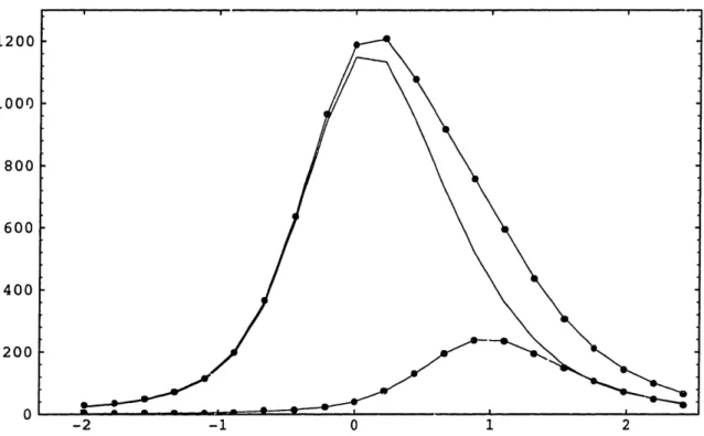
Figure 2.4. Typical Pluto/Charon image (marginal column). A marginal column is the average of all the columns in an image, such as the images of Fig. 2.3. The upper set of points is the raw data (upper left in Fig. 2.3). The lower set of points is the raw data with the model Pluto subtracted (lower left of Fig. 2.3). The lines are (from lowest to highest) the model Charon, the model Pluto, and the sum of the two model PSFs.

Since Midas moved 7 to 12 pixels during an exposure, the PSF was convolved with

Midas' motion to model the elongated image. The "Midas-spread function" was fit to the

Midas images and the unconvolved PSF to the field stars. Because DAOPHOT does not

2.3.2 REGISTRATION OF EXPOSURES

The star centers defined the astrometric relationship between the different exposures. A set of coefficients (aij, bij) linearly converted the rows and columns (r and c) for a given exposure to the transformed rows and columns (rtrans and Ctrans) of a reference frame:

rtrans = ao00 + alOr + a01C (2.2)

Ctrans boo + blor + bol0

We built up the reference frame by minimizing the weighted scatter of each star's transformed positions around its mean transformed position. One exposure was chosen to define the absolute scale of the reference frame; for this exposure, r = rtrans and c = ctrans. The Pluto and Charon positions are transformed to the reference frame as well.

The Midas frames for each night were registered in a similar manner. Since the Midas observations were used to determine the image scale and orientation, the centers of the field stars and Midas were corrected for differential aberration and refraction before the exposures were registered. The differential changes in position were cast as linear equations in row and column, using the linear terms from Green (1985, Eq. (13.24) and (13.32)). Correcting for differential refraction and aberration decreased the image scale by 3 parts in 104 and had no significant effect on the orientation.

reference plane

x

S

-W Y

Figure 2.5. Orbital elements. The apparent ellipse depicted was generated using Charon's orbital elements. The line-of-sight vector is perpendicular to the paper, so this figure depicts Charon's orbit as seen from Earth. The angles indicated are the longitude of the ascending node (), the inclination (i), and the argument of latitude (u). The dots indicate the position of the satellite (S), the ascending node (N), and the origin of the longitude (y).

23.3 MODEL ROWS AND COLUMNS

The first step in calculating the rows and columns of Pluto and Charon is finding the apparent orbit of Charon around Pluto. TB90 found that the eccentricity of Charon's orbit around Pluto was 0.00020+0.00021, unless the line of apsides happens to be along the line of sight, in which case it could be as high as 0.01. The eccentricity is assumed to be

zero for this analysis. The remaining orbital elements, shown in Fig. 2.5, are the

inclination (i), the longitude of the ascending node (), the argument of latitude (u,

identical to TB90's "mean anomaly, measured from the ascending node"), and the

semimajor axis of Charon's orbit around Pluto (a, not shown).

All calculations involving the right ascension (a) and declination (6) are performed in

tangent-plane ("standard") coordinates ( and l ). These are obtained by gnomonic

projection: the projection of the celestial sphere onto a plane tangent at a given right

ascension and declination (ao, 60) (Green 1985, Eq. (13.12)):

cos 6 sin(a - a )

sin 0sin 6 + cos80 cos cos(a - ao)

(2.3)

cos60sin/5 - sin 60cos 6cos(a - ao) sin 60 sin 6 + cosb0cos6 cos(a - ao)

From the orbital elements and the position of the barycenter (ab and 6b), the difference in the standard coordinates of Pluto ((p, rip) and Charon (c, lc) is adequately

defined by:

c

a -sin(ab - Q) cos(b - )cosi os(2.4)

|lc

-

p

A

-cos(c - )sin 8b -sin(a b-

Q2)sin

6bcos i + cos bsin i [sin

u

(2)

where A is the Earth-Pluto distance.

The rotational phase (p) and (under the assumption of a circular orbit) the argument of

latitude increase at a constant rate, starting from initial values po and u0o defined at an

initial Julian date, JDo. If JD is the time of observation, then

u-uo

JD- (A / c) - JDo

= - PO = (2.5)

where c is the speed of light (173 AU/day), and P is the period, for which we adopt 6.387246 0.000011 days from TB90. To compare results with TB90, we use their epoch, JD2446600.5. At 1992 Mar 1 9:53:27 UT, an integral number of orbits had

occurred since JDo, so at that time u = u0 and p = P0 = 0.46111. The phase is calculated

using the definition of Binzel et al. (1985), with the substitution of TB90's value for the

period.

The standard coordinates relative to the barycenter depend on the mass ratio, q:

F P1 = r bl1 q qpJ rp lb + q c qp (2.6) Lec jibe 1 f - lP = I I+ qc

lrb

l

l+q

tic -qp

We generated a light-time corrected, geocentric, J2000 ephemeris of the barycenter at 10-minute intervals from JPL's DE202 ephemeris (Standish 1987) using the SPICELIB

library provided by the NAIF group at JPL (Acton 1990). These were linearly interpolated to the times of observations, and converted to topocentric a and 6. We then calculated Fb and rqb from Eq. (2.3), choosing a tangent point whose J2000 position was

near the center of the CCD: ao = 1 5h 37M 35S, 60 = -4 00' 55".

The standard coordinates were transformed linearly to the row and column of the

reference frame using the plate constants ml 1, ml 2, m21, and m22.

[

=

o] +

2]

x1

i]

(2.7)

The free parameters (q, a, i, 9, u0, mIl , m2, m21, m22, r0, co) were adjusted to minimize

(in a least-squares sense) the difference between the model and observed rows and columns.

2.4. RESULTS

In this section, we apply the model of Section 2.3 to the Pluto and Charon centers. In

the first battery of fits (Table 2.3a), we do not constrain any parameters. We first apply the model to all converged Pluto and Charon centers (Fit #1). The night of February 28 is a poor fit to the model for the following reasons: (i) we will see in Section 2.5 that the position of Charon is particularly sensitive to the shape of the constructed PSF on this nighnt; (ii) the FWHM is large while the separation is small; (iii) only 4 out of 16 exposures converged; and (iv) the errors assigned to the Charon centers on February 28 were seven times larger than on the other nights. When the fitted data do not include February 28 (Fit #2), the mean residuals are much lower, but the mass ratio changes by only a third of its formal error. For the remainder of the paper, we exclude February 28

from the analysis. Fits #3 - 6 include just the first, second, third, or fourth exposure on each frame. Since the four exposures were offset from one another by 10 arcsec, fitting one exposure at a time tests if the results are strongly dependent on the locations of the

images. The average scatter of the parameters for Fits #3 - 6 is close to twice the formal

error of Fit #2, as expected because only one quarter of the data were used. The scatter for q is somewhat higher, at 3.2 times the formal error of Fit #2. We fit for the Pluto positions alone, in Fit #7. In this fit, we need to fix a, because we are effectively fitting for Pluto's orbital semimajor axis, ap = a q ( +q)-'. The amplitude of the Pluto wobble is consistent with Fit #2, but the other elements are not as well determined.

C) BO 0 ' 0 I+ I+ I . f+ I+ j Lu -₄ LAOS ~ ~ ~ ~ ~ ~ _{,4 + 1 4i+9 + 1 ' 14 4}o -(D 0 P C' V 00 C1 (.A- ZJ 0 · 0O0 h.) ~ - o o A 00 : L 00 , w LAO' I~ ~ "~ V~H ' 'H 00 ~ VI LA LA _cD H' L'0 o o !2-0o~o

0 0 LA

-'00tA 1 4 ' 1 Z 1 4 b LA + 4' I ' A 1 4' 1 4 ' 400_a, LA t4. 0 ' IO% _Lit 0 VI + N 0 V, R 1+u O '] 1+ ('+ R FI- I+ H 0 C:) I+

~

14.I _'. , _L ~~00 0~ _{L 0- 0} o h, 00 (n~oo oAr L LAj ,' - ' . u,:..4 oo a~ ,~,, o o h. 00 ₀

_{H H}

_-

_h

0 -_0 i LA . '+ '+ _{P P} LAI00 ₀ o t _PA00 ' o 1+₀

AI

I~\

g

PI

0 0O

C )

o h) O ~

o

4V

L A L~00 _{(~~~~~~~~~~~~~..}-4

0 0 0 0

- t

0

· c OO bo Ln VI - _it~~~~~~~t

W0

-

.

0

'\.\0

0

14 I+ I+ i ' ' 14'

H-

wl 00

H

'

-

o0 L A '. - ! 0 -0 0 0 0 c. J O \ '. 0' 0

0·

0

'.

, ? 0 br O tA bo I W~~~~H H- oo H- 14-A R I+ 00I CD 0

2

1

z

""1 0 O0 00 D- C o o, oI 00_{cr w} CX t.

~00

00 cmz _ocr M U) TI_Cu0'-a '. o o 4 D 00 t3 CD h) LC

t-0

o. (D 0 CD O O c P.. 0

In the second battery of fits (Table 2.3b), we used all the centers except those from the night of February 28, and fixed various parameters. The independently determined

values and errors for the fixed parameters are parenthesized in Table 2.3b. Fit #8 fixes the shape of the orbit by fixing i, uo, and Q at the TB90 orbital elements, precessed to the

J2000 equino . TB90's formal errors in u0 and Q are smaller than those from the imaging

observations of this work (Fit #2) and NOS93. This is true even if we consider the additional 0.20° error in uo that arises from propagating the error in the period forward from JDo. The mutual events are most sensitive to the elements best measured at minimum separation: the timing of the orbit (controlled mainly by uo) and the width of the apparent ellipse (controlled mainly by Q2). In contrast, imaging is more sensitive to those elements measured at elongation: the semimajor axis of the orbit (controlled entirely by a) and the orientation of the apparent ellipse (controlled mainly by i). Fit #9

uses u and Q from TB90. Because Fit #9 is consistent with the unconstrained fit (Fit #2),

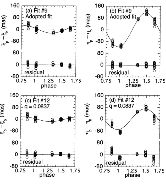
with fewer degrees of freedom, we adopt Fit #9 as our solution.

We can determine the plate constants from the motion of Pluto, the motion of 1981 Midas, and the locations of the field stars. Midas moved in essentially a straight line across the field, providing the image scale and orientation. These are converted to plate

constants (ml 1, ml2, m21, m22) for Fit #10, and adjusted for the differential refraction and

aberration appropriate for the reference frame. For Fit #11, we fixed the plate constants at those determined by an unweighted fit of the mean star positions to the positions found

by the MIT occultation search.

Fits #1 - 11 all give mass ratios much larger than the value of 0.0837 - 0.0147 found by NOS93. Fit #12 demonstrates what happens when we force a small value of q on our observations. The rms Pluto residuals are 40% larger than those for the adopted solution.

O o _o n C CA ' CD (D = _o D C < CD 0 Cg C1 CD a S o \0 S bW LA -I+ I+ § i t

to

o

. .

b

or O \O tz o R _{I+ + I+}

00

0

0

-0

140%

0

OA

W00A~

C It

ob

O o

0% X O _{R 1+ io t-} -_ 8 ° OC° 00 lJi-J

o

X

-4o

o -3 ~' 0I O -I+ It 1

C,

+ I+ 1+ -4

A3

L POh

-00

A (it Ut Io

oo

IX

0

C -

I o W ° -j je -4 00 - + N _ O O O 0 I+ 1+ _{If 1}I) o o I o

VI

P

;-h-(Cg 0 V~j3 4 00

_o

₄

O _ Ao N) 00 o ' IH I+ + I + + + @+ It + 00 0 _

00

W00

It It l I t 0oo '0 o

-H

--I+ I+ I+ I+ j+ O _ O iW b\ be A w\or

Pluto's barycentric orbit and residuals for the adopted solution and for the low-q solution

are shown in Fig. 2.6. For the adopted solution, the nightly means in the residuals of

rp - 1 b are scattered around zero. In contrast, the nightly mean residuals for the low-q

"' W~ - - =1 , , -a 1-a 3 . ,0 B -a . '- I 5i - >< >e' >e _{R _} 4 5, 6 I

1-

_{P , -- a .1 ,} P I _{; P -} "

R.

0

t,

cJ C', 0

i

LD CD 0 o 00 0O o;

O'

0_C; a 9 =1 ₀ T O; Ol 0 a W I, _{_} la pW W 00 00 21 0 2. rl N) 0 Ct I+ O0 It H O -4 O I+ O 0 -O I+ oa 0

z

0

(0 W 1 ... Il -Q

solution are as large as 26 milliarcsec, and the residuals are quantitatively sinusoidal.

Clearly, we did not achieve a good fit when we fixed the mass ratio at such a low value.

The results from this work, TB90, and NOS93 are summarized in Table 2.4. When

comparing with the previous results, note that the elements in TB90 are referred to the

equator of B 1950 and have been precessed to J2000 in this work and NOS93.

Table 2.4. Bulk properties for Pluto and Charon

TB90 NOS93 This Worka

Semimajor axis, a (km) 19640 ± 320 19405 ± 86 19460 ± 58 Inclinationb, i (deg) 99.1 ± 1.0 96.56 ± 0.26 95.00 ± 0.24

Long. of ascending nodeb, 2 (deg) 223.015 ± 0.028 (223.007 ± 0.041) (223.015 ± 0.028)c

Argument of latitudeb, o (deg) 259.76 - 0.08 (260.00 _ 0.24) (259.76 _ 0.08)c

Mass ratio, q - 0.0837 ± 0.0147 0.1566 0.0035

System mass, Msys(102 4g) 14.72 ± 0.72 14.20 + 0.19 14.32 ± 0.13

Pluto mass, Mp (1024g) - 13.10 0.24 12.38 0.12

Charon mass, Mc(1024g) - 1.10 ± 0.18 1.94 + 0.04

a Fit 9

b Referred to the mean equator and equinox of J2000 at epoch JD 2446600.5 c Fixed at value from Tholen and Buic 1990.

The mass ratio is the main goal of this work and NOS93, and the values differ by

nearly a factor of two. However, our semimajor axis is consistent with previous results (where the TB90 value is taken from Beletic et al. 1989). The elements Q and uO were

fixed at the TB90 values in this work. NOS93 describe how they constrained fQ and uo to

be near the TB90 values. Both this work and NOS93 find a smaller inclination than

TB90, although the differences among all three inclinations are larger than the formal

errors. This difference is not due to a real change in the inclination, as the observations of

NOS93 and this work were taken only 6 months apart. The ~0.25° error in the inclination implies an accuracy of about 0.4%, as does the ~70 km error in the semimajor axis. The

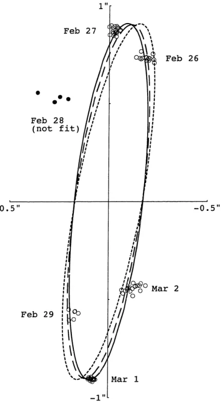
apparent orbit of Charon around Pluto is shown in Fig. 2.7 for all three sets of elements,

-

(a) Fit #9

: Adopted fit

o

resiual V

re,

s

ual

_{, , , , I} 75 1 1.25

phase

160

(a -o E .o I _9w

80

0

-80

80

0

RAn 1.5 1.75

,resiiual

..

I

75 1 1.25

phase

1.5 1.75 I I I ' I (c) Fit #12

-

q =

0.0837

-

residual

I I, ,, I I I I , I j 75 1 1.25

phase

160 0 co E I I

80

0

-80

80

0

1.5 1.75

Iresid

ual , ,

, I ,, , Il,, ,,, 75 1 1.25

phase

1.5 1.75

Figure 2.6. Pluto's distance from the barycenter in the direction of increasing right ascension (p

- b) and increasing declination (ip - rib). Shown are (a) Up - b for the adopted fit, (b) 1lp - ib

for the same fit, (c) Up - (b for the low-q fit, and (d) Tip - lb for the same fit. In the upper portion of each plot, the curve is the model separation and the open circles are the observed separations. The lower portion shows the residuals, at the same vertical scale. Note that the nightly means of the residuals are clustered around zero for the adopted fit, but are as large as 26 milliarcsec

when q is fixed at the value from NOS93.

4 , IOU co E .0 0. ,Jnf

80

0

-80

0

160 C, E -C

J.

I Q,, W~r

80

0

-80

80

0

-. n

r ,, MU I--_ _

-a n

O,v 0.;

0.

O., A ,V 0." _.An.,0., o

Feb 27 0·

00

Feb 28 (not fit) 0. Feb 26 .5"

Figure 2.7. Charon's orbit around Pluto. The solid line is the adopted solution (Fit #9). The open circles are the observations that were included in the fit. The solid circles were excluded. The dashed line is the orbit from NOS93, and the dotted orbit is for TB90. North is up and

east is to the left.

2.5. BOUNDS ON SYSTEMATIC ERRORS

This section investigates possible sources of the difference in the measurement of q

by this work and NOS93. The effect of random errors on the derived mass ratio should be

reflected in its formal error. To the extent they can be modeled, systematic corrections

should not degrade the results. Unmodeled or incorrectly modeled systematic corrections

can lead to an incorrect measurement of the mass ratio. Table 2.5 summarizes the mean

random error, the maximum systematic correction, and the associated error for the

various steps in the analysis.

Table 2.5. Sources of random and systematic error.

Random Error Systematic Effects Comments (milliarcsec) (milliarcsec)

this work NOS93 this work NOS93 this work NOS93 Finding centers

Pluto - 5 - 2 0 3 0 + 0 blended, distinct peaks, Charon + 24 - 8 0 7 10-(3) PSF from field stars PSF from literature Registration - 2 _ 2 0 1 0 - 46 6-10 field stars, 1 field star,

full linear solution same scale for row & col

Field 0 0 0 + 20 89 ± 2 direct imaging reimaging optics

Distortion

Center-of-light 0 0 4 (4) 10±(10) Buie etal. (1992) Buie & Tholen (1989)

# of exposures 80 14

Span of data 78% of orbit 50% of orbit

Both NOS93 and this work found the centers by PSF fitting. The formal errors in the

centers were smaller for NOS93 than for this work, because their PSF had a smaller core.

Balancing this, we use 80 observations for 5 nights spanning 6 nights, compared with

NOS93's 14 observations, spanning 4 nights. PSF fitting can introduce systematic errors;

if the constructed PSF is a bad match to Pluto at the distance of Charon, Charon's center

and brightness are adjusted to compensate. As discussed in Section 4.4 of NOS93, their

model PSF probably was an inexact match to the actual HST PSF. They established the

images constructed from field stars. They found the required systematic correction was

up to 10 milliarcsec for Charon, with no significant effect on Pluto. They do not quote an

error in the correction, but state that "thc larger, well-determined corrections were usually

about twice as large as the corresponding solution scatter and were roughly the same for

different choices of registration stars. Therefore, an average correction from a

combination of several star pairs was selected for Charon centroid calibrations." From

this statement we infer that NOS93's error in the systematic correction to fitted centers

was roughly 3 milliarcsec.

In this work, fits of the model PSF to synthetic "Pluto-Charon" images implied no

systematic correction. Any other result would have been surprising, since the PSF was

itself constructed from the field stars. There may still be an unmodeled systematic effect,

if Pluto or Charon differed significantly from the mean PSF determined from the stellar

images. One such difference is the angular diameter of Pluto, which at 29.4 AU is 0.11

arcsec. For our best images, which have a FWHM of 0.91 arcsec, we can apply the results

of Jones et al. (1988), who find that Pluto's angular diameter increases the FWHM by

0.5%. The telescope tracked at Pluto rates, during which time the stars' centers move 0.02

arcsec on the detector.

We placed an upper limit on the systematic correction to the center-finding algorithm

by fitting Pluto and Charon again, with a different model PSF. The nominal PSF was

described in Section 2.3.1. The second PSF was dominated by star 206, and was

constructed using backgrounds derived from a sky annulus. We found, as did NOS93,

that the Pluto positions were relatively insensitive to changes in the PSF. Pluto centers

changed less than 3 milliarcsec. Charon centers changed by 25 milliarcsec f the

represented the range of reasonable deviation of PSFs from the nominal, then these changes provided the estimate for the systematic error inherent in the PSF fitting.

The semimajor axes of this work and NOS93 differed by only 0.4% and the inclinations by 1.60. This agreement was probably not a coincidental cancellation of errors in the image scale and the center-finding algorithms; as evident in Table 2.3, we found the image scale to much better than this accuracy. This implies that the systematic errors in the Pluto-Charon separations are probably less than 0.4% of the semimajor axis, or 4 milliarcsec. The difference in the mass ratio cannot be explained by a difference in

Charon's orbit because (i) the two studies find similar orbits; and (ii) both studies find that

leaving out the Charon centers increases the formal error, but does not change the mass ratio significantly. Since our tests indicate that Pluto's center is much less sensitive than the separation to changes in the PSF, we believe that the difference in the mass ratio is not due to systematic errors in PSF fitting.

We next consider the effects that stellar aberration, refraction, changes in the tangent point, precession, and nutation have on our registration (Section 2.3.2). Precession and nutation are completely removed by defining and with respect to the equator and equinox of J2000. NOS93 corrected for stellar aberration explicitly, and had no need to correct for refraction. In our work, the registration of exposures implicitly accounted for the linear terms of differential refraction (from the variation in airmass over the field), changes in the tangent point, and aberration. The remaining higher-order terms were less than a milliarcsec. The variation of refractivity with color was important only for star 206, whose position was refracted by about 10 milliarcsec relative to the other stars between the minimum and maximum observed zenith distances. The remaining objects had similar colors, and so their relative positions were not shifted significantly by the variation of refraction with wavelength. In particular, the color of Pluto and Charon over

a rotation did not vary enough to significantly change their positions relative to the other

stars.

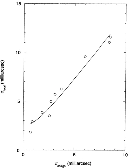
The scatter of the stars' transformed positions provided an estimate of the accuracy of

the registration (Section 2.3.2). Fig. 2.8 shows a plot of this scatter (totai) as a function of

the mean of the formal error assigned by Eq. 2.1 (as.ign). Assuming Eq. 2.1 assigned

appropriate relative weights, the error introduced by the registration (reg) and the ratio of

the true errors to the assigned errors (f) were estimated from total and 0

assign:

2 2 2

JtotaI = Jreg + f assign (2.8)

The best-fit solution (indicated by the curve in Fig. 2.8) implies reg - 2.5 milliarcsec and

fs 1.3.

The concept of "registration error" had to be modified for the NOS93 observations. In

this work, we register the frames to find the positions of Pluto and Charon relative to the field stars. Since there was only one field star present in the NOS93 observations, the

equivalent measurement is the angular distance between the field star and Pluto or

Charon. The random error introduced was the error in the star's position, or 2 milliarcsec.

NOS93 assumed that the scale is constant between exposures, and they quoted a stability

in the scale of 5 parts in 105. Therefore, the systematic errors due to changes in scale with

time were less than 0.1 milliarcsec. A more crucial assumption is that the scale in row or

line (Sy) equals that in column or pixel (Sx). NOS93 adopted a scale ratio (Sy/Sx) of 1.000

_ 0.002. We evaluated the bounds on the systematic errors implied by the error on the

scale ratio; we calculated the Pluto-star separation from Table 4 of NOS93 twice, once

assuming Sy/Sx = 1.000 and again with SylSx = 1.002. The second set of separations was

multiplied by an overall scale change to minimize the difference between the two sets of

.... ' i XI I _ 10 lO aU, E 5 E

5

0 In I I I I I I I I U

0

5

10

assign (milliarcsec)

Figure 2.8. Residuals in the star positions. For each exposure, a linear transformation of centers was found to minimize the scatter of each stars' transformed position. The scatter is shown as a function of the formal error. The curve is the best fit to ctotal2 = reg2 +f 2 assign2, demonstrating that the

random error introduced by the registration is about 2.5 milliarcsec.

I -10

Therefore, the systematic error in NOS93's calculation of the Pluto-star separation is less

than 46 milliarcsec. This is a very loose bound on the systematic error, and could account

for the difference in the measurements of q. However, NOS93 performed one fit with SJSX as a free parameter, and found that q increased by only 1.1 o.

NOS93 have up to 89 milliarcsec of field distortion, mainly from the reimaging optics. They determined the field distortion from 5 overlapping exposures of an open cluster. Their maximum error in the field distortion at the locations of Pluto is

2 milliarcsec.

We expected the field distortion for the UH 2.2-m to be insignificant. The

back-illuminated CCD is mounted in such a way that it is mechanically supported, which should eliminate the "potato chip" warping that was considered by NOS93 (Gerard Luppino, personal communication). In direct imaging mode, the only optical elements are the primary and secondary mirrors, the filter, and the dewar window. Ray-tracing programs for the 2 2-m optics predicted submilliarcsec field distortions for a range of focus positions (Richard Wainscoat, personal communication).

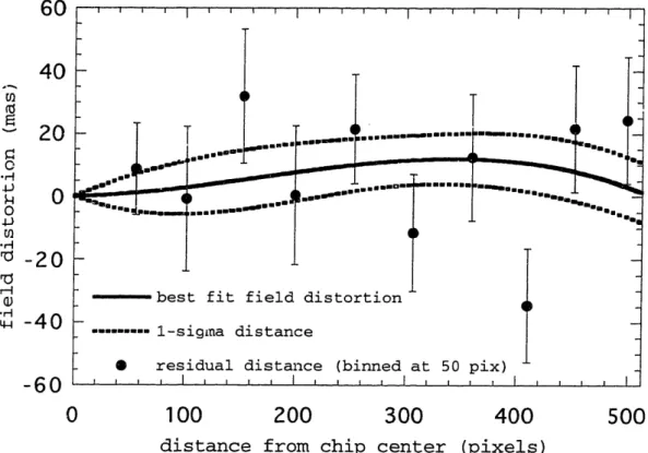
Although our field distortion is expected to be negligible, we need to place observational limits on this. We have five nights of Midas moving from one comer of the field to the opposite corner, which we used to find an image scale and orientation

(Section 4). We use the differences between the observed and predicted Midas centers to fit for a field distortion. As the centers follow essentially one path across the field, we can

fit for field distortions only along that path. The residual distance (Ad) is the difference

between the observed distance (d) and the predicted distance. The residuals were fit with a third order radial function (Eichhorn 1974, Section 2.3.7):

The results of the fit are shown in Fig. 2.7. There is no apparent field distortion, but we can place only a relatively loose bound of -20 milliarcsec.

60

40

M r_ 0 .H CZ

c

-IJ 0 uo rl 4H₀₎ -HI 20 0

-20

-40

-60

0

100

200

300

distance from chip center

400

(pixels)

500

Figure 2.9. Field distortion from Midas observations. The 1-s limit of the fit to the field

distortion is observed to be less than 20 milliarcsec.

Other assumptions in the model led to small systematic errors. The correction from the observed center of light of Pluto to the desired center of disk depends on the albedo distribution assumed for Pluto. The size of the center-of-light offset is 4 milliarcsec; this serves as a reasonable bound on the uncertainty in position introduced by the model-dependent nature of the albedo maps. Uncertainties in the starting times of the exposures corresponded to errors of 0.01 milliarcsec. Errors in the ephemeris during one week of observation can be simply treated as an offset. The mutual events constrain the

eccentricity of Charon's orbit only if the longitude of periapse is not along the line of sight. If it is, the eccentricity could be as high as 0.01, which would introduce a systematic error of 5 milliarcsec.

CHAPTER 3

OCCULTATIONS BY SMALL-PLANET ATMOSPHERES*

3.1 INTRODUCTION

The definitive detection of Pluto's atmosphere occurred on 1988 June 9, when

starlight dimmed gradually as it was occulted by Pluto (Fig. 3.1). The upper portion of

the occultation light curve has the shap- characteristic of an occultation by an isothermal

atmosphere, but just below half light is a kink where the light curve becomes steeper.

Previous analysis of this occultation assumed an isothermal atmosphere that was clear

above the kink, while the lower portion has been explained by an absorbing haze layer

(Elliot et al. 1989) or a steep thermal gradient (Eshleman 1989; Hubbard et al. 1990).

Calculations of radiative heating and cooling by methane predict the region above the

drop should be isothermal (Hubbard et al. 1990; Yelle and Lunine 1989). The detection

of, or limits on, a thermal gradient in this region would provide a test of this prediction.

To make such a detection, we needed a light-curve model for a non-isothermal

atmosphere. Goldsmith (1963) derived a light-curve model for an atmosphere with a

linear thermal profile. Unfortunately, this model is not valid for Pluto because it assumes

that the scale height is much smaller than the radius of the region probed. In this

"large-planet" limit, the following are ignored: (i) variable gravity; (ii) focusing of the starlight

in the plane perpendicular to the direction of propagation; and (iii) variation of the radius

during the occultation compared with the radius itself. These effects are of the same

order as the effects of the thermal gradient we were trying to detect. This requires us to

derive a model that includes a thermal gradient and all the small-planet effects.

* Chapter 3 and Appendix I are exerpted from the paper Elliot, J. L., and L. A. Young 1992. Analysis of stellar occultation data for planetary atmospheres. I. Model fitting, with application to Pluto. Astron. J.

X r-I h r1

Hr-q

~

.

a) U) (a - S -->

isothermi

or

mild gradi haze

or

inversioi

curve in the absence of haze or inversion

h

S,

time

Figure 3.1. Anatomy of Pluto's stellar occultation light curve. Signal level is plotted versus time for the immersion portion of an occultation light curve, from the start of the occultation to the midtime. At the start of the occultation, the flux is at its unocculted level, sf, and drops to the background level, Sb, at mid-occultation. The upper portion has the shape characteristic of an atmosphere with at most a mild thermal gradient. If the atmosphere did not experience some sort of transition, the lightcurve would follow the dashed line. At the time t = tim + Th,l, the Pluto occultation has a sharp drop. The times when the stellar flux has dropped to half its unocculted value (tim and tem) correspond to the "half-light" radius on the planet. The time corresponding to optical depth = 1 of an assumed haze is also indicated.

Analyses of occultation light curves by atmospheres rely on the equations relating the

observed flux to the refractivity profile. In numerical inversions of the light curve, the

refractivity profile is obtained directly from the data, and is then related to the thermal

profile by assuming hydrostatic equilibrium. In least-squares fitting, one specifies the

functional form of the temperature and local scale height; hydrostatic equilibrium is again

assumed, and the flux-refractivity relations are used to produce a synthetic light curve.

I will first present the equations for the flux in terms of arbitrary functions of temperature,

local scale height, and linear extinction coefficient. These equations are the starting point

_ ___

for generating any synthetic stellar occultation light curve (Baum and Code 1953; Elliot

et al. 1989; Elliot and Young 1992; Goldsmith 1963).

I apply these general equations to the specific problem of a small planet with a haze layer and thermal and compositional gradients. This leads to equations written in terms of the physical characteristics of the atmosphere (such as the refractivity and linear absorption coefficient) and the occultation geometry (such as the observer-body distance

or the observer's position in the shadow as a function of time).

To perform least-squares fitting, one would like a set of parameters that have low correlations and whose relationship to the light curve is easily visualized. I describe one such set, and how to convert between the "atmospheric" parameters (used for deriving the light curve) and the "data" parameters (used for least-squares fitting).

3.2 GENERAL FLUX EQUATION

Fig. 3.2 illustrates light from a star being occulted by a planetary atmosphere. Monochromatic, parallel light rays are incident on a planetary atmosphere from the left and then encounter a spherically symmetric planet. The center of the occulting planet's shadow lies on the line that is parallel to the incoming light rays and passes through the center of the planet. The "observer's plane" is the plane that contains the observer and is perpendicular to the incident light rays. The observer's position is described by the observer-planet distance, D, and the distance from the center of the shadow in the observer's plane, p.

A light ray with closest approach distance r to the center of the planet is bent by the atmosphere and then deviates from its original path by an angle 0(r), remaining in the plane containing the center of the planet and the original path of the ray. This ray

dr

Planet Plane Observer's Plane

Figure 3.2. Occultation by a planetary atmosphere. Starlight encounters a planetary atmosphere and is bent by the gradient of refractivity in the atmosphere. Since the refraction increases exponentially with depth in the atmosphere, two neighboring rays separate, causing the star to dim as seen by a distant observer. Another dimming effect is atmospheric extinction, which exists in our model only for radii less than rl.

intersects the planet plane at a radius r and the observer plane at a radius p. The

refraction angle is negative, since rays bend toward the center of the planet, and we

assume it is a small angle for the purpose of trigonometric approximations. If there is

enough bending, or if the observer is far enough from the planet, the ray will arrive at the

observer's plane on the far side of the shadow center. The light from this ray is called the

far-limb contribution to the flux, and it is generally much less than the near-limb

contribution. Since p would never be negative, we have the following relation between

the intersection points of a light ray in the two planes of interest:

The stellar flux will be changed by three effects upon passing through the planetary

atmosphere: (i) differential bending of the light rays; (ii) absorption by the atmosphere;

and (iii) partial focusing of the light by the curvature of the planetary limb in the plane

perpendicular to the path of the ray. An initial bundle of light rays that has a width dr

before interaction with the planet will be expanded into a width dp in the observer's plane, due to differential bending. This decreases the stellar flux by the factor Idrldpi. Atmospheric absorption diminishes the flux by a factor exp[-Tcb(r)], where %TbS(r) is the observed optical depth along the path of the ray. Finally, the focusing by the planetary limb increases the flux by the ratio of the circumferences of the "circles of light" of radius

r and p. Hence, the flux in the observer's plane, E(r), is simply written as a product of

three factors:

(r) =

r

dr

exp[-Tbs(r)]= exp -TobS(r)] (3.2)

- (r) dp~r)

D(r)

+

I

D

dO(r)

Eq.

(3.2)

describes

the

a single

contribution

from

limb.

To nd

the

normalized

stelladr

Eq. (3.2) describes the contribution from a single limb. To find the normalized stellar flux, j(p), in the observer's plane, we sum the single limb flux, t(r), for all values of r that would arrive at p. We assume the only contribution to the flux is from the near limb, so [p(r)] = 4(r). This implies there is no ray crossing, and we can write Eqs. (3.1) and (3.2) without taking absolute values. With this assumption, the observed normalized flux

is:

(p) = ex[- bs(r)] (3.3)

(I +

D

O(rr)

( + D(r)

The flux as defined is normalized so that it equals one in the absence of an occultation. The normalized flux is multiplied by the signal that would have been received by the unocculted star, s(t), then added to the background signal, sb(t), that