Increased light-use efficiency in northern terrestrial ecosystems indicated by CO 2 and greening observations

(1)

HAL Id: hal-02922775

https://hal.archives-ouvertes.fr/hal-02922775

Submitted on 17 Sep 2020

HAL is a multi-disciplinary open access

archive for the deposit and dissemination of

sci-entific research documents, whether they are

pub-lished or not. The documents may come from

teaching and research institutions in France or

abroad, or from public or private research centers.

L’archive ouverte pluridisciplinaire HAL, est

destinée au dépôt et à la diffusion de documents

scientifiques de niveau recherche, publiés ou non,

émanant des établissements d’enseignement et de

recherche français ou étrangers, des laboratoires

publics ou privés.

Rebecca Thomas, Iain Colin Prentice, Heather Graven, Philippe Ciais, Joshua

Fisher, Daniel Hayes, Maoyi Huang, Deborah Huntzinger, Akihiko Ito, Atul

Jain, et al.

To cite this version:

Rebecca Thomas, Iain Colin Prentice, Heather Graven, Philippe Ciais, Joshua Fisher, et al..

In-creased light-use eﬀiciency in northern terrestrial ecosystems indicated by CO 2 and greening

obser-vations. Geophysical Research Letters, American Geophysical Union, 2016, 43 (21), pp.11,339-11,349.

�10.1002/2016GL070710�. �hal-02922775�

(2)

Increased light-use eﬃciency in northern terrestrial

ecosystems indicated by CO

₂

and greening

observations

Rebecca T. Thomas1,2,3_{, Iain Colin Prentice}2,4_{, Heather Graven}3,4_{, Philippe Ciais}5_{, Joshua B. Fisher}6_, Daniel J. Hayes7_{, Maoyi Huang}8_{, Deborah N. Huntzinger}9_{, Akihiko Ito}10_{, Atul Jain}11_{, Jiafu Mao}12_, Anna M. Michalak13_{, Shushi Peng}14_{, Benjamin Poulter}15_{, Daniel M Ricciuto}12_{, Xiaoying Shi}12_, Christopher Schwalm16_{, Hanqin Tian}17_{, and Ning Zeng}18

1_{Science and Solutions for a Changing Planet DTP, Imperial College London, London, UK,}2_{AXA Chair Programme in}

Biosphere and Climate Impacts, Department of Life Sciences, Imperial College London, London, UK ,3_{Department of}

Physics, Imperial College London, London, UK,4_{Grantham Institute: Climate Change and the Environment, Imperial}

College London, London, UK,5_{Laboratoire des Sciences du Climat et de l’Environnement, Saint-Aubin, France,} 6_{Jet Propulsion Laboratory, California Institute of Technology, Pasadena, California, USA,}7_{School of Forest Resources,}

University of Maine, Orono, Maine, USA,8_{Atmospheric Sciences and Global Change Division, Paciﬁc Northwest National}

Laboratory, Richland, Washington, USA,9School of Earth Sciences and Environmental Sustainability, Northern Arizona University, Flagstaﬀ, Arizona, USA,10_{Center for Global Environmental Research, National Institute for Environmental}

Studies, Tsukuba, Japan,11_{Department of Atmospheric Sciences, University of Illinois at Urbana-Champaign, Urbana,}

Illinois, USA,12_{Climate Change Science Institute and Environmental Sciences Division, Oak Ridge National Laboratory,}

Oak Ridge, Tennessee, USA,13_{Department of Global Ecology, Carnegie Institution for Science, Stanford, California, USA,} 14_{Sino-French Institute for Earth System Science, College of Urban and Environmental Sciences, Peking University, Beijing,}

China,15_{Department of Ecology, Montana State University, Bozeman, Montana, USA,}16_{Woods Hole Research Center,}

Falmouth, Massachusetts, USA,17International Center for Climate and Global Change Research, School of Forestry and Wildlife Sciences, Auburn University, Auburn, Alabama, USA,18_{Department of Atmospheric and Oceanic Science and}

Earth System Science Interdisciplinary Center, University of Maryland, College Park, Maryland, USA

Abstract

Observations show an increasing amplitude in the seasonal cycle of CO₂(ASC) north of 45∘N of 56 ± 9.8% over the last 50 years and an increase in vegetation greenness of 7.5–15% in high northern latitudes since the 1980s. However, the causes of these changes remain uncertain. Historical simulations from terrestrial biosphere models in the Multiscale Synthesis and Terrestrial Model Intercomparison Project are compared to the ASC and greenness observations, using the TM3 atmospheric transport model to translate surface ﬂuxes into CO2concentrations. We ﬁnd that the modeled change in ASC is too small

but the mean greening trend is generally captured. Modeled increases in greenness are primarily driven by warming, whereas ASC changes are primarily driven by increasing CO2. We suggest that increases

in ecosystem-scale light use eﬃciency (LUE) have contributed to the observed ASC increase but are underestimated by current models. We highlight potential mechanisms that could increase modeled LUE.

1. Introduction

Observations show that the terrestrial biosphere is responding to anthropogenic environmental change [Friedlingstein et al., 2014; Ciais et al., 2014]. Photosynthetic CO2uptake currently exceeds release through

res-piration and other processes, and the terrestrial biosphere removes around a quarter of anthropogenic CO2

emissions each year [Ciais et al., 2014]. Net uptake of CO2can be partly attributed to “CO2fertilization,” since

increases in ambient CO2can increase the biochemical rate of photosynthesis and increase water use

eﬃ-ciency [Franks et al., 2013; Penuelas et al., 2011; Keenan et al., 2013]. Net uptake of CO2may also result in part

from changes in climate, land management, ecosystem composition, and N deposition, among other factors [Huntzinger et al., 2013]. Better understanding of how the terrestrial biosphere has responded to changes in climate, CO₂, and other drivers over recent years is needed to understand how it might change in the future and whether it will continue to serve as a net sink [Le Quere et al., 2015; Friedlingstein et al., 2006; Schimel

et al., 2015]. In this paper we compare long-term observations of atmospheric CO2and greenness to terrestrial

biosphere model output.

RESEARCH LETTER

10.1002/2016GL070710

Key Points:

• Current terrestrial biosphere models underestimate northern CO₂seasonal cycle amplitude increase

• Models capture observed greening trends and therefore increased uptake of light by ecosystems

• Reconciling these suggests an increase in ecosystem light use eﬃciency larger than models simulate

Supporting Information: • Supporting Information S1 Correspondence to: R. T. Thomas, r.thomas14@imperial.ac.uk Citation:

Thomas, R. T., et al. (2016), Increased light-use eﬃciency in northern terrestrial ecosystems indicated by CO₂and greening observations, Geophys. Res. Lett., 43, 11,339–11,349, doi:10.1002/2016GL070710.

Received 23 JAN 2016 Accepted 12 OCT 2016

Accepted article online 15 OCT 2016 Published online 4 NOV 2016

(3)

The seasonal cycle of CO₂in the Northern Hemisphere can be almost entirely attributed to terrestrial bio-sphere exchange [Randerson et al., 1997; Graven et al., 2013], so changes in the seasonal cycle of CO₂indicate large-scale changes in northern terrestrial ecosystem exchange. Increases in the amplitude of the seasonal cycle of CO₂(ASC) have been observed at the measurement stations Mauna Loa, Hawaii (Mauna Loa Observa-tory (MLO)), and Point Barrow, Alaska (BRW) of 0.32±0.07% yr−1_{and 0}_{.60±0.05% yr}−1_{, respectively, since the}

early 1960s [Keeling et al., 1996; Graven et al., 2013]. Recently, Graven et al. [2013] measured long-term changes in ASC throughout the higher latitudes of the Northern Hemisphere. Comparisons between two aircraft campaigns in 1958–1961 and 2009–2011 showed an increase in ASC of 5.0±0.8 ppm (56±9.8%) between 45 and 90∘N at 500 mb, indicating that the seasonal uptake and release of CO2in terrestrial ecosystems between

30 and 90∘N increased by 32–59% over this time [Graven et al., 2013]. The largest contribution to the ASC was in the main growing season[Graven et al., 2013]. Increases in ASC may therefore be related to the extratropical net carbon sink as studies suggest that increases in net terrestrial carbon uptake during the growing season drive the northern extratropical net carbon sink [Rayner et al., 2015; Gurney and Eckels, 2011].

Vegetation greenness, deﬁned here as the fraction of photosynthetically active radiation that is absorbed by green vegetation on land (fAPAR), has been measured by satellites since mid-1981 [Murray-Tortarolo et al., 2013]. An increase of vegetation greenness has been observed between 30 and 90∘N of 8.7% for all types of vegetation from 1982 to 2010 (Figures 4b and S3b in the supporting information). These trends imply that photosynthetic activity in northern latitudes has increased over the last three decades [Slayback et al., 2003;

Zhu et al., 2013]. Many studies attribute greening primarily to rising temperature in spring and autumn, leading

to a reduction in snow cover, an earlier start to the growing season [Piao et al., 2008; Myneni et al., 1997; Notaro

et al., 2005; Xu et al., 2013] and increased peak greenness [Buitenwerf et al., 2015; Myneni et al., 1997].

Observations of the CO2seasonal cycle and vegetation greenness, and their changes over time, present

opportunities to evaluate terrestrial biosphere models. Reproducing the mean CO2seasonal cycle requires

that modeled photosynthesis and respiration have the correct phase and magnitude. Reproducing the changes in ASC additionally requires that interactions between the terrestrial biosphere and the environmen-tal drivers, including climate, CO2, land use, and disturbance (e.g., ﬁre and insects), are well represented in

models [Mcguire et al., 2001]. Previous comparisons have shown that the long-term increase in ASC observed in the aircraft data was underestimated by the coupled carbon-climate CMIP5 Earth System Models [Graven

et al., 2013], whereas the smaller trend observed in ASC at ground-based NOAA stations over 1982–2011

was captured by one off-line dynamic vegetation model (LPJml). In LPJml, the ASC increase was primarily driven by increases in vegetation cover and plant productivity resulting from increasing temperatures at high latitudes [Forkel et al., 2016]. However, other studies that examined seasonal biosphere fluxes have found conflicting results. For the off-line terrestrial biosphere models taking part in the Multiscale Synthesis Terres-trial Model Intercomparison Project (MsTMIP) and the TRENDY dynamic vegetation model intercomparison project, changes in seasonal fluxes were predominately driven by climate change in only a minority of models. In most current biosphere models, the increase in atmospheric CO₂is the primary driver of changes in sea-sonal fluxes [Ito et al., 2016; Zhao et al., 2016]. In comparisons of observed and modeled greening trends, the TRENDY models suggest that greening has been primarily driven by climate change at higher northern latitudes (60–90∘N) and by CO₂at lower northern latitudes (30–60∘N) [Zhu et al., 2016].

There is a clear need to identify mechanisms that reconcile observed and modeled changes in ASC and greening and to clarify the role of CO2, climate change, and other factors driving ecosystem changes. A key

distinction can be made between changes in the structure (leaf area) and the physiology (intrinsic rate of carbon uptake) of vegetation by using the concept of light use eﬃciency (LUE), the net primary productivity (NPP) per unit of light absorbed (APAR) [Norby et al., 2003]. If increases in NPP for a given ecosystem were driven solely by increased leaf area, and therefore increased APAR, NPP would relate to APAR by a constant factor corresponding to the LUE of the ecosystem. However, increases in NPP may also arise from increases in LUE, even in the absence of APAR increases. A decade of plot-scale observations from four temperate sites in the Free Air CO2Enrichment experiments show that in medium- to high-density canopies, increases in NPP

were driven by LUE increases, while there was no signiﬁcant change in APAR [Norby et al., 2003; McCarthy

et al., 2006; Long et al., 2004]. Analysis of LUE trends in models can therefore help to elucidate mechanisms of

ecosystem change and to inform model-data comparisons of fAPAR and CO₂exchange [Norby et al., 2005]. In this paper, we compare observed changes in ASC and greening trends to output from 13 biosphere models in MsTMIP, applying the concept of LUE to interpret the model-data comparison. In MsTMIP, the process-based

(4)

terrestrial biosphere models ran semifactorial experiments where photosynthesis and respiration were driven by a standard set of observed changes in climate, land use, CO₂, and in some cases N deposition [Huntzinger

et al., 2013; Wei et al., 2014]. We compare modeled output of greenness to the longest available record of

satellite fAPAR data—fPAR3g [Zhu et al., 2013]. We use the TM3 atmospheric transport model with net ecosys-tem production from MsTMIP to evaluate the modeled seasonal cycle amplitude of atmospheric CO2directly

against aircraft measurements in 1958–1961 and 2009–2010. The aircraft data are more representative of large-scale behavior than surface measurement stations [Sweeney et al., 2015; Keppel-Aleks et al., 2012; Sawa

et al., 2012], showing a clearer and more consistent signal. Thus, aircraft data are a stronger constraint on

large-scale ecosystem changes than the long-term records at the surface stations MLO and BRW, but they have previously been compared only with CMIP5 models [Graven et al., 2013].

We show that most MsTMIP models simulate overall greening trends well but underestimate the observed ASC change. Increases in modeled NPP in northern ecosystems are a combination of CO2-driven increases

in LUE and climate-driven greening. Since models capture greening trends but underestimate the change in ASC, we suggest that models underestimate increases in ecosystem LUE over the past several decades and we discuss potential causes for this phenomenon.

2. Methodology

2.1. Observed Data

2.1.1. Seasonal Amplitude of Atmospheric CO₂

The aircraft campaigns “International Geophysical Year” in 1958–1961 and “HIAPER Pole-to-Pole Observa-tions” in 2009–2011 observed atmospheric CO₂in the middle to lower troposphere [Graven et al., 2013]. We focus on the change in the amplitude of the seasonal cycle of CO₂(ASC) at 500 mb in the 45–90∘N region, where the largest increase in ASC was observed: 5.0 ± 0.8 ppm (56 ± 9.8%). We do not consider phase shifts in the CO2seasonal cycle, since they are not clearly resolved either by aircraft observations [Graven et al., 2013]

or monthly model output.

2.1.2. Vegetation Greenness

Vegetation greenness was analyzed using the remotely sensed third-generation fAPAR data product, fPAR3g, at 1/12∘ resolution [Zhu et al., 2013]. The data were averaged to the 0.5∘ × 0.5∘grid of the MsTMIP models over 1982–2011 [Zhu et al., 2013]. Monthly fAPAR was calculated as the mean of 15 day cloud-free composites, then weighted by average monthly PAR per grid cell and summed for months with a temperature above 0∘C to get annual growing season fAPAR (GS-fAPAR). Total GS-fAPAR was calculated as the mean of all land grid cells north of 30∘N. See Text S1 for full methods.

2.2. Model Output 2.2.1. MsTMIP Models

We analyze CO₂ﬂuxes from 13 terrestrial biosphere models in the MsTMIP V1.0 experiments (Table S1) [Huntzinger et al., 2014]. Global monthly model output is at 0.5∘ × 0.5∘resolution. Analysis was carried out on years overlapping with the aircraft and satellite observation periods: 1958–1961 and 2009–2010, and 1982–2010 respectively. A standard protocol and environmental driver data set were used to spin-up models to steady state, and control simulations were run for each model with environmental drivers held at preindus-trial levels. Experiments were run in which historical climate, land use change (LUC), and CO2were sequentially

included as model drivers and then N deposition for BIOME-BGC, CLM4, CLM4VIC, DLEM, ISAM, and TEM6 [Huntzinger et al., 2013]. The historical drivers consist of observed and reanalysis data. A land cover map was reinterpreted by each modeling team, for use as the LUC driver [Wei et al., 2014]. Since the models are driven by the same data, intermodel differences reflect how terrestrial biosphere processes have been represented in each model [Dalmonech and Zaehle, 2013; Le Quere et al., 2015; Huntzinger et al., 2013; Sitch et al., 2015]. Unless otherwise stated, the simulation including all time-varying historical drivers is used in the results. We also analyze individual contributions to fluxes from climate, LUC, CO2or N deposition, which were calculated

as the difference between the first simulation in which that type of historical data was used and the previous simulation. One model, BIOME-BGC, only ran the “climate-only” and “all-on” experiments, with fixed LUC and N deposition.

Monthly net ecosystem productivity (NEP) was calculated from model outputs as the difference between net primary production and heterotrophic respiration (NPP-Rh) [Chapin et al., 2006]. This neglects fire and other disturbances that are often absent or poorly represented in models and poorly constrained by obser-vations [Huntzinger et al., 2013]. The CO2concentration resulting from the NEP fluxes was calculated for each

(5)

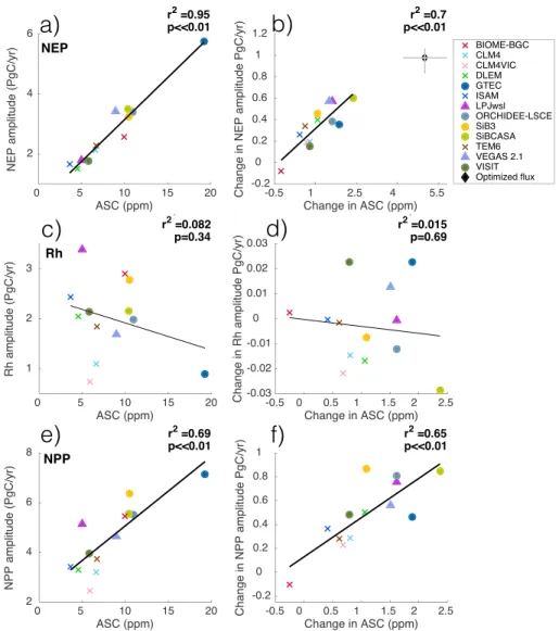
Figure 1. Observed and modeled ASC by latitude for (a) 1958-61, (b) 2009-10 and (c) diﬀerence between 2009-10 and 1958-61. Model type depicted by markers: no nitrogen cycle, no dynamic vegetation (circles), no nitrogen cycle, dynamic vegetation (triangles), and nitrogen cycle, no dynamic vegetation (crosses). Grey shading is observational uncertainty from [Graven et al., 2013].

model and simulation using the TM3 atmospheric transport model at 5∘ × 3.83∘ resolution, forced by National Centers for Environmental Prediction reanalysis data speciﬁc for each year [Heimann and Korner, 2003]. This captures any changes in atmospheric transport, even though transport eﬀects were shown to have little impact on long-term ASC trends [Graven et al., 2013]. Compared to other atmospheric transport models, TM3 does not show large biases in seasonal CO2amplitude or vertical exchange [Gurney et al., 2004; Stephens et al.,

2007]. The simulated CO2concentration from NEP was added to simulated CO2concentrations from monthly

ocean [Patra et al., 2011; Roedenbeck et al., 2003] and fossil fuel [Andres et al., 2011] ﬂuxes for the same years. The total CO2concentration for each model was then detrended for each latitude band using a polynomial

ﬁt, and the mean CO2concentration was subtracted and interpolated to aircraft data at 500 mb.

Monthly modeled fluxes of NPP, Rh, and NEP were each summed over 30–90∘N for 1958–1961 and 2009–2010, and the seasonal amplitude and mean annual flux was calculated for each flux and time period. The flux and CO2concentration amplitudes were calculated as the difference between the maximum and

minimum of the mean seasonal cycle.

Modeled leaf area index (LAI, the projected area of leaves over an area of ground [Murray-Tortarolo et al., 2013]) was converted to fAPAR using the Beer’s Law approximation:

fAPAR = 1 − e−0.5LAI_. ₍₁₎

Modeled GS-fAPAR was calculated in the same way as observed GS-fAPAR (section 2.1.2). Modeled growing season LUE was calculated for land 30–90∘N in 1958–1961 and 2009–2010 as

GS-LUE = GS-NPP

GS-APAR, (2)

where

GS-APAR = GS-fAPAR × PAR. (3)

3. Results

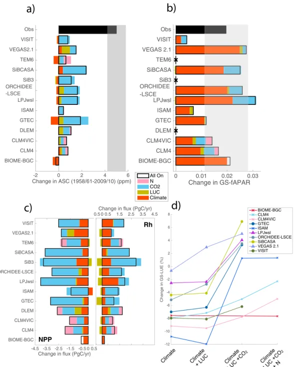
3.1. Seasonal CO2Amplitude Change

MsTMIP models are generally able to reproduce the amplitude of the CO2seasonal cycle and its latitudinal

gra-dient at 500 mb in 1958–1961 but not in 2009–2010 (Figure 1). Models simulate a wide range of ASC change north of 45∘N, −0.5 to 2.4 ppm, all substantially lower than observed (Figures 1 and S2). The models generally

(6)

Figure 2. ASC in 2009–2010 compared to percentage change in ASC from 1958–1961 to 2009–2010 for aircraft observations (black square), MsTMIP models (colored markers), and CMIP5 models for TM3 only (grey markers) (revised from [Graven et al., 2013]). Grey shading is observational uncertainty [Graven et al., 2013].

capture the phase of the CO2seasonal cycle (Figure S3a). The primary driver of the increase in modeled ASC is

CO₂(Figure 4). Coupled carbon-nitrogen cycle (C-N) models have among the smallest changes in ASC and the weakest CO2-driven increases. The small CO2-driven ASC increase in C-N models is likely due to N limitation,

as ASC further increases in simulations when time-varying N deposition is included. LPJwsl is the only model that has a fractional increase in ASC within the observational uncertainty (47%) (Figure 2), but its absolute ASC and ASC change are much too small (Figure 1). The ASC change in the MsTMIP models is similar to the CMIP5 models [Graven et al., 2013, Figure 2], although MsTMIP models tend to have smaller 2009–2010 amplitudes.

3.2. Vegetation Greenness

Models are generally able to reproduce the observed interannual variability in GS-fAPAR and its increase of 0.02 (8.7%) between 30 and 90∘N from 1982 to 2010 (Figures 4b and S3b). Observed and modeled greening was due to an increase in leaves per unit area, rather than vegetated area. Only ISAM showed an increase in vegetated area. All models show that greening is driven by climate (Figure 4b), and models perform best in arctic and boreal regions where greening trends have been driven by increasing temperatures [Piao et al., 2006] (Figure S1). There is little inﬂuence on the overall greening trend from LUC, CO2, and N deposition.

These drivers may be of more importance at lower latitudes where models do not match observed trends well (Figure S1) and where greening trends depend more on how vegetation is represented in models [Eastman

et al., 2013; Murray-Tortarolo et al., 2013; Zhu et al., 2016].

3.3. Terrestrial Carbon Fluxes 3.3.1. NEP

The amplitude of NEP varies from less than 1 Pg C k yr−1_{to more than 5 Pg C yr}−1_{, consistent with previous}

studies showing MsTMIP models have high intermodel variability in NEP, as well as in its constituent ﬂuxes, gross primary production, and ecosystem respiration [Huntzinger et al., 2013; Zscheischler et al., 2014; Schwalm

et al., 2015]. NEP amplitude generally increased (Figure 3b), as shown previously for MsTMIP [Ito et al., 2016]

and TRENDY [Zhao et al., 2016]. NEP amplitude is well correlated to the simulated ASC across the models;

r2_{= 0}_{.95 (Figure 3a). There is also a good correlation between NEP amplitude change and ASC change}

(Figure 3b), though somewhat weaker (r2_{= 0}_{.70), which may be due to additional inﬂuences on ASC change}

from ﬂuxes south of 30∘N.

Figure 3b also shows the optimized ﬂux of NEP, from Graven et al. [2013], where NEP amplitude in arctic, boreal, and temperate regions were adjusted to best match the pattern of observed ASC change in aircraft and surface data. The optimized increase in NEP amplitude from Graven et al. [2013] is larger than any modeled increase, but it lies within the uncertainty of the model regression line, indicating that the relationship between ASC and NEP amplitude change is similar.

(7)

Figure 3. Modeled ASC and amplitude of (a) NEP, (c), NPP and (e) Rh for 2009–2010. This relationship is similar in 1959–1961. Modeled ASC change and change in amplitude of (b) NEP, (d) NPP, and (f ) Rh. All panels except Figure 3b show fluxes for land 30∘N–90∘N and ASC for 45∘N–90∘N at 500 mb and regression lines are plotted, with markers as in Figure 1. In Figure 3b, NEP is for arctic, boreal, and temperate regions only, defined by the biome mask in Graven et al. [2013]. The black diamond is observed ASC change and optimized flux of NEP from Graven et al. [2013].

3.3.2. Rh

There is no signiﬁcant correlation between modeled Rh amplitude and ASC or between Rh amplitude change and ASC change (r2_{≈ 0) (Figures 3e and 3f ); thus, changes in Rh cannot be driving the change in modeled}

NEP amplitude and ASC. Mean annual Rh increased, but changes in Rh amplitude were small because Rh increased throughout the year rather than in the month of maximum Rh (Figures 3f and 4c). The small changes in MsTMIP Rh amplitude are inconsistent with CMIP5 models, which show much larger Rh amplitude changes [Graven et al., 2013, Figure S9], perhaps due to climate feedbacks in CMIP5 models that are not present in the oﬀ-line MsTMIP models.

The largest increase in mean annual Rh is generally from CO₂, although climate is dominant in VEGAS, LPJwsl, and N deposition is dominant in CLM4VIC and CLM4 (Figure 4c).

3.3.3. NPP

The modeled seasonal amplitude of NPP and change in NPP amplitude are signiﬁcantly correlated to mod-eled ASC and change in ASC across the models; r2 _{= 0}_{.69 and r}2 _{= 0}_{.65, respectively (Figures 3c and 3d).}

Mean annual NPP and seasonal NPP amplitude increased for all models between the two periods (except NPP amplitude in BIOME-BGC) (Figure 4c). Hence, changes in modeled NPP, not Rh, are driving the change in modeled NEP amplitude and ASC.

(8)

Figure 4. Contributions from climate, LUC, and CO₂N deposition to modeled changes in (a) ASC, (b) GS-fAPAR, (c) mean annual NPP and Rh, and (d) GS-LUE. ASC is for 45∘N–90∘N at 500 mb between 1958–1961 and 2009–2010 (Figure 4a). Fluxes are for 30∘N–90∘N between 1982–2010 (Figure 4b) and 1958–1961 to 2009–2010 (Figures 4 and 4d). Fluxes are positive into the atmosphere. In Figure 4a, observations and uncertainty (grey shading) are from [Graven et al., 2013]. In Figure 4b, the 95% conﬁdence interval in the observed trend is shown (grey shading). LAI was not available for DLEM and TEM6, and LAI was assimilated from remote sensing for SiB3, so no output is shown in Figures 4b or 4d for these models.

CO2is the primary driver of NPP increase for most models, while climate and LUC generally result in smaller

changes in NPP (Figure 4c). Changes in NPP and NPP amplitude are smallest in C-N models, resulting in small NEP and ASC change (Figures 3b and 4a).

3.4. Light Use Eﬃciency

Models show mixed results for the overall change in GS-LUE (−7.8 to 6.9%, Figure 4d), but the sign of the LUE response to climate change is consistent across models. Climate change decreases GS-LUE in all models, while

(9)

increasing CO₂increases GS-LUE in all models. Increases in LUE result from N deposition in CLM4 and CLM4VIC, and from LUC in VEGAS2.1 and ORCHIDEE-LSCE, while LUC has little inﬂuence on LUE in the other models. Figure 4 shows that CO2is driving increases in modeled NPP, which results in increases in GS-LUE and ASC.

On the other hand, while NPP and greening are also increasing with climate change, this does not translate to increased GS-LUE or ASC.

4. Discussion and Conclusion

Current terrestrial biosphere models simulate greening trends reasonably well, but the large increase in observed ASC at high latitudes remains unexplained. There is little difference in simulated ASC or ASC change between models driven with prescribed climate and CO₂[Zhao et al., 2016; this study], or with modeled climate as in CMIP5 [Graven et al., 2013] (Figure 2), indicating that the disagreement between observations and models lies in the modeling of terrestrial biosphere processes rather than in the climatic forcing. Consistent with previous studies [Graven et al., 2013; Randerson et al., 1997], Figure 3 implies that modeled increases in NEP amplitude lead to increases in modeled ASC. Furthermore, our model-based results suggest NPP as the main driver of NEP amplitude change, also consistent with previous studies [Randerson et al., 1997; Forkel et al., 2016; Zhao et al., 2016]. NEP changes may also be influenced by respiration or disturbance [Zimov et al., 1999], but these effects must be secondary to NPP [Houghton, 1987; Randerson et al., 1997; Graven et al., 2013; Forkel

et al., 2016]. Since the MsTMIP models underestimate ASC changes, they are likely also to have underestimated

increases in the seasonal amplitude of NPP.

Since NPP can increase through vegetation greening (increased APAR) and/or through an increase in ecosys-tem LUE (equation (2)), the models’ ability to capture the greening trends, and the absence of a trend in PAR (Figure S5), suggests that discrepancies with observed ASC result primarily from errors in the models’ representation of LUE. In particular, we suggest that models are capturing the increase in NPP in the early growing season through climate-driven greening but underestimating the GS-LUE-driven increase in NPP in the peak of the growing season when canopies are denser. Our model-data comparison thus provides strong evidence for an increase in GS-LUE across ecosystem in high northern latitudes that is larger than simulated by MsTMIP models.

Increased LUE relates to physiological changes that enhance NPP in addition to, or in the absence of, structural changes through increased leaf area. NPP can increase through CO₂fertilization, as elevated CO₂increases photosynthesis and water use eﬃciency [Ainsworth and Long, 2005; Norby et al., 2003]. CO₂fertilization is included in the MsTMIP models [Huntzinger et al., 2013], and it is the primary driver of simulated NPP increases (Figure 4c). In models, CO2fertilization plays a key role during the peak growing season when canopies

are more dense, as seen in Figure 4 in which CO2-driven NPP increases correspond to GS-LUE and ASC

increases. Large uncertainties remain regarding the magnitude of the CO2fertilization eﬀect [Smith et al., 2016;

Schimel et al., 2015], but studies agree that N dynamics are a key, and often missing, component of this eﬀect

[Terrer et al., 2016; Wieder et al., 2015].

Climate change may aﬀect photosynthesis and respiration in ways that are not well represented in MsTMIP models, particularly through temperature acclimation of photosynthesis and autotrophic respiration (Ra), and through carbon allocation and nutrient availability. Ra acclimates to sustained higher temperatures faster than photosynthesis [Ryan and Law, 2005; Way and Oren, 2010; Reich et al., 2016], potentially increasing the fraction of photosynthesis that results in NPP. The only two MsTMIP models that allow for Ra temperature acclimation, LPJwsl and VISIT, have among the largest climate-driven increases in absolute NPP (Figure 4c). Ra acclimation was also included in the LPJml model, which was shown to reproduce the increase in ASC at ground-based stations [Sitch et al., 2003; Forkel et al., 2016]. Warming has also been shown to increase above-ground allocation of carbon [Poorter et al., 2012; Way and Oren, 2010; Melillo et al., 2011], potentially due to accelerated cycling of N through the soil that reduces the requirement for belowground carbon allocation [Melillo et al., 2011; Wieder et al., 2015]. Most MsTMIP models do not include N cycling, and C-N models may underestimate this eﬀect. Aboveground carbon allocation could also drive structural changes that increase leaf area and contribute to greening, depending on the species and on ecosystem conditions [Ainsworth and

Long, 2005; Way and Oren, 2010; Melillo et al., 2011; McCarthy et al., 2006].

Recent studies have suggested that land use change (LUC) could be responsible for a substantial portion of the ASC increase [Gray et al., 2014; Zeng et al., 2014]. Speciﬁcally, the transition from forest to intensive

(10)

high-yielding crops could increase ASC because such crops can have more concentrated growing seasons and higher NPP than forests [Gray et al., 2014]. In MsTMIP models, LUC is not a large contribution to ASC change (Figure S4), accounting for −8 to 47% of the increase in modeled ASC (Figure 4a). MsTMIP models may not be adequately representing LUC since most models do not explicitly represent crops or land management (Table S1). However, the LPJml model used by [Forkel et al., 2016] does explicitly include crops and also ﬁnds a small contribution to ASC change from LUC (7%) [Forkel et al., 2016]. LUC is unlikely to explain much of the large diﬀerences between models and observations in any case, particularly because most LUC has been at 30–45∘N [Gray et al., 2014], south of the boreal forest region that contributes the most to observed ASC changes [Graven et al., 2013]. Other vegetation changes, such as the observed northward shift of the tree line [Harsch et al., 2009; Elmendorf et al., 2012], may have increased NPP at higher latitudes. This shift is an important driver of the increased ASC in LPJml [Forkel et al., 2016] but may not be captured by MsTMIP models. Several factors may be contributing to the observed increase in ASC over the last 50 years. We conclude that a key factor is an increase in LUE that is larger than simulated by current models. Warming and increases in atmospheric CO2may have caused stronger increases in LUE than in the MsTMIP models through a

combina-tion of CO2fertilization, respiration acclimation, increases in the rate of N cycling, and a shift to aboveground

carbon allocation. Improving the modeled LUE response to CO2and climate change is important not only

for process-based models such as those participating in MsTMIP but also for diagnostic models that use satellite-derived fAPAR to estimate NPP. This study highlights that combining atmospheric CO2measurements

and observed greening trends provides a powerful constraint on terrestrial biosphere models, particularly through the analysis of structural and physiological ecosystem changes using the light use eﬃciency concept and should be included in future model benchmarking exercises.

References

Ainsworth, E. A., and S. P. Long (2005), What have we learned from 15 years of free-air CO₂enrichment (FACE) a meta-analytic review of the responses of photosynthesis, canopy, New Phytol., 165(2), 351–371.

Andres, R. J., J. S. Gregg, L. Losey, G. Marland, and T. A. Boden (2011), Monthly, global emissions of carbon dioxide from fossil fuel consumption, Tellus, Ser. B, 63(3), 309–327.

Buitenwerf, R., L. Rose, and S. I. Higgins (2015), Three decades of multi-dimensional change in global leaf phenology, Nat. Clim. Change, 5(4), 364–368.

Chapin, I., et al. (2006), Reconciling carbon-cycle concepts, terminology, and methods, Ecosystems, 9(7), 1041–1050.

Ciais, P., et al. (2014), Carbon and other biogeochemical cycles, in Climate Change 2013: The Physical Science Basis. Contribution of Working Group I to the Fifth Assessment Report of the Intergovernmental Panel on Climate Change, edited by T. F. Stocker et al., pp. 465–570, Cambridge Univ. Press, Cambridge, U. K., and New York.

Dalmonech, D., and S. Zaehle (2013), Towards a more objective evaluation of modelled land-carbon trends using atmospheric CO₂and satellite-based vegetation activity observations, Biogeosciences, 10(6), 4189–4210.

Eastman, J. R., F. Sangermano, E. A. Machado, J. Rogan, and A. Anyamba (2013), Global trends in seasonality of normalized diﬀerence vegetation index (NDVI), 1982–2011, Remote Sens., 5(10), 4799–4818.

Elmendorf, S. C., et al. (2012), Plot-scale evidence of tundra vegetation change and links to recent summer warming, Nat. Clim. Change, 2(6), 453–457.

Forkel, M., N. Carvalhais, C. Rodenbeck, R. Keeling, M. Heimann, K. Thonicke, S. Zaehle, and M. Reichstein (2016), Enhanced seasonal CO₂ exchange caused by ampliﬁed plant productivity in northern ecosystems, Science, 351(6274), 696–699.

Franks, P. J., et al. (2013), Sensitivity of plants to changing atmospheric CO2concentration: From the geological past to the next century,

New Phytol., 197(4), 1077–1094.

Friedlingstein, P., et al. (2006), Climate–carbon cycle feedback analysis: Results from the (CMIP)-M-4 model intercomparison, J. Clim., 19(14), 3337–3353.

Friedlingstein, P., M. Meinshausen, V. K. Arora, C. D. Jones, A. Anav, S. K. Liddicoat, and R. Knutti (2014), Uncertainties in CMIP5 climate projections due to carbon cycle feedbacks, J. Clim., 27(2), 511–526.

Graven, H. D., et al. (2013), Enhanced seasonal exchange of CO₂by northern ecosystems since 1960, Science, 341(6150), 1085–1089. Gray, J. M., S. Frolking, E. A. Kort, D. K. Ray, C. J. Kucharik, N. Ramankutty, and M. A. Friedl (2014), Direct human inﬂuence on atmospheric

CO₂seasonality from increased cropland productivity, Nature, 515(7527), 398–401.

Gurney, K. R., and W. J. Eckels (2011), Regional trends in terrestrial carbon exchange and their seasonal signatures, Tellus, Ser. B, 63(3), 328–339.

Gurney, K. R., et al. (2004), Transcom 3 inversion intercomparison: Model mean results for the estimation of seasonal carbon sources and sinks, Global Biogeochem. Cycles, 18, GB1010, doi:10.1029/2003GB002111.

Harsch, M. A., P. E. Hulme, M. S. Mcglone, and R. P. Duncan (2009), Are treelines advancing? A global meta-analysis of treeline response to climate warming, Ecol. Lett., 12(10), 1040–1049.

Heimann, M., and S. Korner (2003), The global atmospheric tracer model TM3: Model description and user’s manual, release 3.8a, Tech. Rep., Max-Planck-Inst. for Biogeochemistry, Jena, Germany.

Houghton, R. A. (1987), Biotic changes consistent with the increased seasonal amplitude of atmospheric CO₂concentrations, J. Geophys. Res., 92(D4), 4223–4230.

Huntzinger, D., et al. (2014), NACP MSTMIP: Global 0.5-deg Terrestrial Biosphere Model Outputs (Version 1) in Standard Format, Oak Ridge Natl. Lab. Distrib. Active Arch. Cent., Oak Ridge, Tenn.

Huntzinger, D. N., et al. (2013), The north american carbon program multi-scale synthesis and terrestrial model intercomparison project–Part 1: Overview and experimental design, Geosci. Model Dev., 6(6), 2121–2133.

Acknowledgments

This work was supported by the Grantham Institute: Climate Change and the Environment–Science and Solutions for a Changing Planet DTP, grant NE/L002515/1 and is a contri-bution to the AXA Chair Programme in Biosphere and Climate Impacts. All data used for this analysis are publicly available with full sources detailed in the supporting information. We thank Peter Rayner and an anonymous reviewer for their helpful comments on the manuscript. Funding for the Multiscale synthesis and Terrestrial Model Intercomparison Project (MsTMIP; http://nacp.ornl.gov/ MsTMIP.shtm) activity was provided through NASA ROSES grant NNX10AG01A. Data management support for preparing, documenting, and distributing model driver and output data was performed by the Modeling and Synthesis Thematic Data Center at Oak Ridge National Laboratory (ORNL; http://nacp.ornl.gov), with funding through NASA ROSES grant NNH10AN681. Finalized MsTMIP data products are archived at the ORNL DAAC (http://daac.ornl.gov). Biome-BGC code was provided by the Numerical Terradynamic Simulation Group at University of Montana. The computational facilities were provided by NASA Earth Exchange at NASA Ames Research Center. CLM4 and GTEC simulations were supported in part by the U.S. Department of Energy (DOE), Office of Science, Biological and Environmental Research. Oak Ridge National Laboratory is managed by UTBATTELLE for DOE under contract DE-AC05-00OR22725. CLM4-VIC research is supported in part by the U.S. Department of Energy (DOE), Office of Science, Biological and Environmental Research. PNNL is operated for the U.S. DOE by BATTELLE Memorial Institute under contract DE-AC06-76RLO1830. DLEM developed in International Center for Climate and Global Change Research, Auburn University has been supported by NASA Interdisciplinary Science Program (IDS), NASA Land Cover/Land Use Change Program (LULUC),NASA Terrestrial Ecology Program, NASA Atmospheric Composition Modeling and Analysis Program (ACMAP), NSF Dynamics of Coupled Natural-Human System Program (CNH), Decadal and Regional Climate Prediction using Earth System Models (EaSM), DOE National Institute for Climate Change Research, USDA AFRI Program, and EPA STAR program. LPJwsl work was conducted at LSCE, France, using a modified version of LPJ version 3.1 model, originally made available by the Potsdam Institute for Climate Impact Research. ORCHIDEE is a global land surface model developed

(11)

Ito, A., et al. (2016), Decadal trends in the seasonal-cycle amplitude of terrestrial CO₂exchange resulting from the ensemble of terrestrial biosphere models, Tellus, Ser. B, 68, 28968, doi:10.3402/tellusb.v68.28968.

Keeling, C. D., J. F. S. Chin, and T. P. Whorf (1996), Increased activity of northern vegetation inferred from atmospheric CO₂measurements, Nature, 382(6587), 146–149.

Keenan, T. F., D. Y. Hollinger, G. Bohrer, D. Dragoni, J. W. Munger, H. P. Schmid, and A. D. Richardson (2013), Increase in forest water-use eﬃciency as atmospheric carbon dioxide concentrations rise, Nature, 499(7458), 324–327.

Keppel-Aleks, G., et al. (2012), The imprint of surface ﬂuxes and transport on variations in total column carbon dioxide, Biogeosciences, 9(3), 875–891.

Le Quere, C., et al. (2015), Global carbon budget 2014, Earth Syst. Sci. Data, 7(1), 47–85.

Long, S. P., E. A. Ainsworth, A. Rogers, and D. R. Ort (2004), Rising atmospheric carbon dioxide: Plants face the future, Annu. Rev. Plant Biol., 55, 591–628.

McCarthy, H. R., R. Oren, A. C. Finzi, and K. H. Johnsen (2006), Canopy leaf area constrains CO₂-induced enhancement of productivity and partitioning among aboveground carbon pools, Proc. Natl. Acad. Sci. U.S.A., 103(51), 19,356–19,361.

Mcguire, A. D., et al. (2001), Carbon balance of the terrestrial biosphere in the twentieth century: Analyses of CO₂, climate and land use eﬀects with four process-based ecosystem models, Global Biogeochem. Cycles, 15(1), 183–206.

Melillo, J. M., et al. (2011), Soil warming, carbon-nitrogen interactions, and forest carbon budgets, Proc. Natl. Acad. Sci. U.S.A., 108(23), 9508–9512.

Murray-Tortarolo, G., et al. (2013), Evaluation of land surface models in reproducing satellite-derived LAI over the high-latitude northern hemisphere. Part I: Uncoupled DGVMS, Remote Sens., 5(10), 4819–4838.

Myneni, R. B., C. D. Keeling, C. J. Tucker, G. Asrar, and R. R. Nemani (1997), Increased plant growth in the northern high latitudes from 1981 to 1991, Nature, 386(6626), 698–702.

Norby, R. J., J. D. Sholtis, C. A. Gunderson, and S. S. Jawdy (2003), Leaf dynamics of a deciduous forest canopy: No response to elevated CO₂, Oecologia, 136(4), 574–584.

Norby, R. J., et al. (2005), Forest response to elevated CO₂is conserved across a broad range of productivity, Proc. Natl. Acad. Sci. U.S.A., 102(50), 18,052–18,056.

Notaro, M., Z. Y. Liu, R. Gallimore, S. J. Vavrus, J. E. Kutzbach, I. C. Prentice, and R. L. Jacob (2005), Simulated and observed preindustrial to modern vegetation and climate changes, J. Clim., 18(17), 3650–3671.

Patra, P. K., Y. Niwa, T. J. Schuck, C. A. M. Brenninkmeijer, T. Machida, H. Matsueda, and Y. Sawa (2011), Carbon balance of south asia constrained by passenger aircraft CO₂measurements, Atmos. Chem. Phys., 11(9), 4163–4175.

Penuelas, J., J. G. Canadell, and R. Ogaya (2011), Increased water-use eﬃciency during the 20th century did not translate into enhanced tree growth, Global Ecol. Biogeogr., 20(4), 597–608.

Piao, S., P. Friedlingstein, P. Ciais, L. Zhou, and A. Chen (2006), Eﬀect of climate and CO₂changes on the greening of the northern hemisphere over the past two decades, Geophys. Res. Lett., 33, L23402, doi:10.1029/2006GL028205.

Piao, S., et al. (2008), Net carbon dioxide losses of northern ecosystems in response to autumn warming, Nature, 451(7174), 49–53. Poorter, H., K. J. Niklas, P. B. Reich, J. Oleksyn, P. Poot, and L. Mommer (2012), Biomass allocation to leaves, stems and roots: Meta-analyses of

interspeciﬁc variation and environmental control, New Phytol., 193(1), 30–50.

Randerson, J. T., M. V. Thompson, T. J. Conway, I. Y. Fung, and C. B. Field (1997), The contribution of terrestrial sources and sinks to trends in the seasonal cycle of atmospheric carbon dioxide, Global Biogeochem. Cycles, 11(4), 535–560.

Rayner, P. J., A. Stavert, M. Scholze, A. Ahlstrom, C. E. Allison, and R. M. Law (2015), Recent changes in the global and regional carbon cycle: Analysis of ﬁrst-order diagnostics, Biogeosciences, 12(3), 835–844.

Reich, P. B., K. M. Sendall, A. Stefanski, X. R. Wei, R. L. Rich, and R. A. Montgomery (2016), Boreal and temperate trees show strong acclimation of respiration to warming, Nature, 531(7596), 633–636.

Roedenbeck, C., S. Houweling, M. Gloor, and M. Heimann (2003), Time-dependent atmospheric CO₂inversions based on interannually varying tracer transport, Tellus, Ser. B, 55(2), 488–497.

Ryan, M. G., and B. E. Law (2005), Interpreting, measuring, and modeling soil respiration, Biogeochemistry, 73(1), 3–27.

Sawa, Y., T. Machida, and H. Matsueda (2012), Aircraft observation of the seasonal variation in the transport of CO₂in the upper atmosphere, J. Geophys. Res., 117, D05305, doi:10.1029/2011JD016933.

Schimel, D., B. B. Stephens, and J. B. Fisher (2015), Eﬀect of increasing CO₂on the terrestrial carbon cycle, Proc. Natl. Acad. Sci. U.S.A., 112(2), 436–441.

Schwalm, C. R., et al. (2015), Toward “optimal” integration of terrestrial biosphere models, Geophys. Res. Lett., 42, 4418–4428, doi:10.1002/2015GL064002.

Sitch, S., et al. (2003), Evaluation of ecosystem dynamics, plant geography and terrestrial carbon cycling in the LPJ dynamic global vegetation model, Global Change Biol., 9(2), 161–185.

Sitch, S., et al. (2015), Recent trends and drivers of regional sources and sinks of carbon dioxide, Biogeosciences, 12(3), 653–679.

Slayback, D. A., J. E. Pinzon, S. O. Los, and C. J. Tucker (2003), Northern hemisphere photosynthetic trends 1982–99, Global Change Biol., 9(1), 1–15.

Smith, W. K., S. C. Reed, C. C. Cleveland, A. P. Ballantyne, W. R. L. Anderegg, W. R. Wieder, Y. Y. Liu, and S. W. Running (2016), Large divergence of satellite and earth system model estimates of global terrestrial CO₂fertilization, Nat. Clim. Change, 6(3), 306–310.

Stephens, B. B., et al. (2007), Weak northern and strong tropical land carbon uptake from vertical proﬁles of atmospheric CO₂), Science, 316(5832), 1732–1735.

Sweeney, C., et al. (2015), Seasonal climatology of CO₂across north America from aircraft measurements in the NOAA/ESRL global greenhouse gas reference network, J. Geophys. Res. Atmos., 120, 5155–5190, doi:10.1002/2014JD022591.

Terrer, C., S. Vicca, B. A. Hungate, R. P. Phillips, and I. C. Prentice (2016), Mycorrhizal association as a primary control of the CO₂fertilization eﬀect, Science, 353(6294), 72–74.

Way, D. A., and R. Oren (2010), Diﬀerential responses to changes in growth temperature between trees from diﬀerent functional groups and biomes: A review and synthesis of data, Tree Physiol., 30(6), 669–688.

Wei, Y., et al. (2014), The north american carbon program multi-scale synthesis and terrestrial model intercomparison project—Part 2: Environmental driver data, Geosci. Model Dev., 7(6), 2875–2893.

Wieder, W. R., C. C. Cleveland, W. K. Smith, and K. Todd-Brown (2015), Future productivity and carbon storage limited by terrestrial nutrient availability, Nat. Geosci., 8(6), 441–444.

Xu, L., et al. (2013), Temperature and vegetation seasonality diminishment over northern lands, Nat. Clim. Change, 3(6), 581–586. Zeng, N., F. Zhao, G. J. Collatz, E. Kalnay, R. J. Salawitch, T. O. West, and L. Guanter (2014), Agricultural green revolution as a driver of

increasing atmospheric CO₂seasonal amplitude, Nature, 515(7527), 394–397. at the IPSL institute in France. The

simulations were performed with the support of the GhG Europe FP7 grant with computing facilities provided by “LSCE” or “TGCC.” SiB3 research was carried out at the Jet Propulsion Laboratory, California Institute of Technology, under a contract with the National Aeronautics and Space Administration. TEM6 research is sup-ported in part by the U.S. Department of Energy (DOE), Oﬃce of Science, Biological and Environmental Research. Oak Ridge National Laboratory is managed by UT-BATTELLE for DOE under contract DE-AC05-00OR22725. VISIT was developed at the National Institute of Environmental Studies, Japan. This work was mostly conducted during a visiting stay at Oak Ridge National Laboratory. This study was supported by KAKENHI Grand No. 26281014 by the Japan Society of Promotion of Science.

(12)

Zhao, F., et al. (2016), Role of CO₂, climate and land use in regulating the seasonal amplitude increase of carbon ﬂuxes in terrestrial ecosystems: A multimodel analysis, Biogeosciences Discuss., 13, 5121–5137.

Zhu, Z., et al. (2016), Greening of the Earth and its drivers, Nature Clim. Change, 6, 791–795.

Zhu, Z. C., J. Bi, Y. Z. Pan, S. Ganguly, A. Anav, L. Xu, A. Samanta, S. L. Piao, R. R. Nemani, and R. B. Myneni (2013), Global data sets of vegetation leaf area index (LAI)3g and fraction of photosynthetically active radiation (FPAR)3g derived from global inventory modeling and mapping studies (GIMMS) normalized diﬀerence vegetation index (NDVI3g) for the period 1981 to 2011, Remote Sens., 5(2), 927–948.

Zimov, S. A., S. P. Davidov, G. M. Zimova, A. I. Davidova, F. S. Chapin, M. C. Chapin, and J. F. Reynolds (1999), Contribution of disturbance to increasing seasonal amplitude of atmospheric CO₂, Science, 284(5422), 1973–1976.

Zscheischler, J., et al. (2014), Impact of large-scale climate extremes on biospheric carbon ﬂuxes: An intercomparison based on MsTMIP data, Global Biogeochem. Cycles, 28, 585–600, doi:10.1002/2014GB004826.