HAL Id: hal-01668186
https://hal.inria.fr/hal-01668186
Submitted on 19 Dec 2017
HAL is a multi-disciplinary open access
archive for the deposit and dissemination of
sci-entific research documents, whether they are
pub-lished or not. The documents may come from
teaching and research institutions in France or
L’archive ouverte pluridisciplinaire HAL, est
destinée au dépôt et à la diffusion de documents
scientifiques de niveau recherche, publiés ou non,
émanant des établissements d’enseignement et de
recherche français ou étrangers, des laboratoires
On the Stability of Functional Maps and Shape
Difference Operators
Ruqi Huang, Frédéric Chazal, Maks Ovsjanikov
To cite this version:
Ruqi Huang, Frédéric Chazal, Maks Ovsjanikov. On the Stability of Functional Maps and Shape
Difference Operators. Computer Graphics Forum, Wiley, 2017, pp.1 - 12. �10.1111/cgf.13238�.
�hal-01668186�
Volume 0(1981), Number 0 pp. 1–12 COMPUTER GRAPHICSforum
On the Stability of Functional Maps
and Shape Difference Operators
R. Huang1and F. Chazal1and M. Ovsjanikov2
1DataShape, INRIA 2LIX, Ecole Polytechnique
N
M
T
f
1V (f
1)
f
2V (f
2)
(a)
(b)
M
T
N
˜
N
k = 100
k = 50
k = 30
Figure 1: (a) Given two shapes M, N and a map T between them, the functional operator V is generated as one of the shape difference operators introduced in [?]. Intuitively, the real-valued function f2, which is supported on a region that undergoes deformation via T , is significantly distorted by V . Whereas f1, being supported in area-preserved region, remains the same after V acting on it. (b) Given perturbed shapes N to ˜N, we generate highlighted functions with the multi-scale framework of [?], which takes high values (indicated by warm color) in the significantly distorted region. In our paper we prove two types of consistency: horizontally, as the scale k increases, the highlighted functions remain stable, i.e., the regions where high function value takes place are consistent; vertically, at each scale, the highlighted functions are stable with respect to the changes of the input shapes.
Abstract
In this paper, we provide stability guarantees for two frameworks that are based on the notion of functional maps – the shape difference operators introduced in [?] and the framework of [?] which is used to analyze and visualize the deformations be-tween shapes induced by a functional map. We consider two types of perturbations in our analysis: one is on the input shapes and the other is on the change inscale. In theory, we formulate and justify the robustness that has been observed in practical implementations of those frameworks. Inspired by our theoretical results, we propose a pipeline for constructing shape differ-ence operators on point clouds and show numerically that the results are robust and informative. In particular, we show that both the shape difference operators and the derived areas of highest distortion are stable with respect to changes in shape representation and change of scale. Remarkably, this is in contrast with the well-known instability of the eigenfunctions of the Laplace-Beltrami operator computed on point clouds compared to those obtained on triangle meshes.
Categories and Subject Descriptors(according to ACM CCS): I.3.3 [Computer Graphics]: —Shape Analysis.
1. Introduction
Shape comparison is a fundamental problem in geometry process-ing. In the most general setting, this problem consists of encod-ing and quantifyencod-ing similarities and differences across pairs or collections of shapes. This can be especially useful for shape re-trieval [?,?], interpolation [?,?], or visualization [?]. However, even when a map between shapes is given, encoding and visualizing the
differences between them is still challenging. Approaches based on the point-to-point correspondences usually suffer from issues such as sensitivity to noise, difficulty of selecting an appropriate scale of analysis and inconvenient visualization. The discrete nature of point correspondences is one of the major reasons of these issues. The framework of functional maps, which is introduced in [?], alle-viates these issues to some extent by considering more general lin-ear mappings between functions, which can be encoded in a
multi-c
scale fashion with functional bases. As demonstrated in [?], func-tional maps provide a compact, informative representation, which can naturally incorporate tools from spectral analysis.
Based on the notion of functional maps, several approaches have been proposed to analyze pairs or collections of shapes along with maps between them. In this paper we consider two of them, which are intimately related to each other. One is the framework of shape difference operatorsintroduced in [?], which encodes the differ-ences between a pair of shapes as linear operators acting on the functions on one of the shapes (see Figure1(a) for an illustration of one of the operators). And the other is proposed in [?], which generates a collection of multi-scale distortion functions indicating the areas on one of the shapes which undergo deformations. The latter framework can be integrated into the former in the sense that its output, which is a set of highlighted functions, correspond, in essence, to eigenfunctions of shape difference operators.
Though the theoretical formulations of both frameworks are well-established, the associated stability analyses remain absent. In practice, however, we observe the robustness of the outcomes of these frameworks. For example, as shown in Figure1(b), two types of consistency are evidenced: horizontally, as the highlighted func-tions are consistent with respect to the change in scale; vertically, at fixed scales, the highlighted functions are stable with respect to the changes of the input shapes. In this paper, we initiate a rigorous theoretical analysis of these stability properties. In particular, our contributions are three-fold:
• We provide the first rigorous formulations and theoretical guar-antees of stability properties of the shape difference operators. • We propose a new multi-scale scheme for extracting information
from the shape difference operators, which comes with rigorous stability guarantees.
• Inspired by our theoretical results, we design a practical pipeline for computing the shape difference operators on shapes rep-resented by point clouds, and we show numerically that this pipeline is relevant and robust, even when individual spectral quantities such as eigenfunctions of the Laplace-Beltrami oper-ator might not be.
1.1. Overview
We assume that we are given a pair M and N of connected, compact, smooth shapes without boundary. Given a map T : M → N, the au-thors of [?] introduce a pair of linear operators acting on real-valued functions on N, each of which captures one type of differences or distortion between the two shapes induced by T . We first study the stability of these operators with respect to perturbations on metrics and measures on M and on N (Section4).
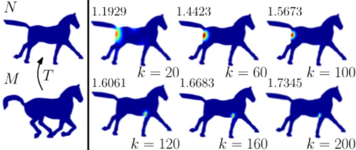
Then we consider the multi-scale framework based on shape dif-ference operators. For one of the shape difdif-ference operators – V as illustrated in Figure1(a), the authors of [?] propose a functional for evaluating the deviation from a function on N to its image un-der V and search for a function that maximizes the functional as a distortion indicator. Then they introduce a multi-scale framework by restricting the search to a subspace spanned by the first k eigen-functions of the Laplace-Beltrami operator (LBO) on N. Figure2
shows typical outputs of this framework: a collection of multi-scale
1.1929 1.4423 1.5673
1.6061 1.6683 1.7345
N
M
T
k = 20
k = 60
k = 100
k = 120
k = 160
k = 200
Figure 2: While being more and more localized with increasing k, the functions from k= 20 to 100 consistently highlight the hip of the horse, whereas the ones from k= 120 to 200 highlight the root of its front right leg. The corresponding quantitative measurements of distortion are marked above of each shape.
highlighted functions on the shape N and a sequence of the corre-sponding maxima of the energy functional shown above the high-light functions with respect to different scales ranging from k = 20 to 200. In this example, we observe consistency in the output at different scales, which are similar to the observations from Fig-ure1(b). Therefore, in the second part of our analyses (Section5), we provide a rigorous stability analysis with respect to the change in scale. One challenge, however, is that the scale in the original framework is controlled by an integer k, and as we will demon-strate in Section5.1, the discrete nature of scale is not suitable for stability analysis. Indeed, as we show below, the result might not be stable with respect to changes of k. To overcome this issue, we introduce a new multi-scale framework whose scale is controlled by a continuous parameter C ∈ R+, and discuss the connection be-tween the two multi-scale frameworks in Section5.4. Within this continuous multi-scale framework, we provide rigorous theoretical guarantees of the stability with respect to C.
Moreover, at any fixed scale C, we prove that the new multi-scale framework is stable with respect to perturbations on the input shapes as well. Figure3illustrates this property: we perturb the input shapes and show the highlighted functions at the same scale k= 50. Note both the stability of the highlighted regions and the proximity among the maxima of the distortion energy shown above the meshes.
(a) Original (b) Densified (c) Simplified 1.2897 1.2947 1.2857
Figure 3: Highlighted functions at a fixed scale for different meshes. We densify the original shape (a) by adding points in the body of the horse (b) and simplify it by down-sampling the limbs (c). The corresponding distortion energy values are shown above.
As an extension, we adapt the other shape difference operator – the one capturing conformal distortion – to the multi-scale frame-work of [?] and prove the stability of this extension with respect to the change in scale as well (Section5.5).
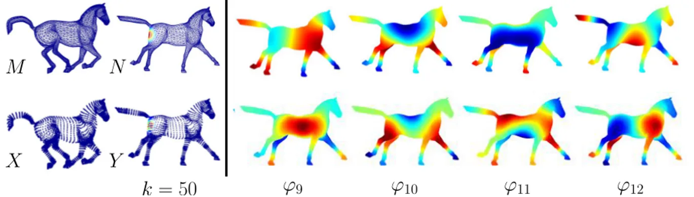
Lastly, we notice that in practice the two frameworks have so far only been constructed on shapes which are discretized as triangle meshes. In Section6.3we extend these constructions by design-ing a pipeline for computdesign-ing shape difference operators on shapes represented as point clouds. As shown in Figure4, although the eigenfunctions of the LBO generated on the mesh N and on the point cloud Y are distinct, the highlighted function generated with M, N are comparable with the one from comparing X ,Y at a fixed scale. This supports the stability results we obtain in theory, and suggests a remarkable robustness of measures based on functional maps and the derived shape difference operators.
To summarize, we provide a rigorous theoretical justification for the stability of shape difference operators in the continuous set-ting. We also propose a new functional sub-domain construction, which we show to be more stable than the classical truncation of eigenspace, in particular leading to provably stable solutions of cer-tain energy functionals used for highlighting distorted regions. Fi-nally, we demonstrate the relevance of our pipeline by applying the shape difference operators to point clouds, which suggests the pos-sibility of extending the existing frameworks to deal more general geometric objects.
1.2. Paper Organization
After discussing related works in Section2, we introduce the pre-liminaries and the notations in Section3. We then study the stabil-ity of shape difference operators in Section4, and provide stability analysis for the framework of [?], by analyzing the perturbations of scale, in Section5.2(Figure2) and of the shapes in Section5.3
(Figure3). We present experimental results showing the stability properties in Section6.
2. Related Work
The two frameworks we analyze in this paper are based on the no-tion of funcno-tional maps, which has been a key ingredient of various applications in geometry processing, including analyzing maps be-tween shapes [?], vector field processing [?, ?] and image segmen-tation [?] to name a few.
Our main focus is to perform perturbation analysis on both shape difference operators (which are linear operators, see [?] for an in-troduction of perturbation analysis on them) and a spectral method based on such operators. Closely related to our analysis is the framework of [?], whose authors conduct perturbation analysis on eigenspace with respect to the Laplace-Beltrami operator on shapes with missing parts. The spectral methods have long been applied in various areas: spectral clustering [?], shape analysis [?] and so on. Besides demonstrating practical usefulness of the spectral meth-ods, providing theoretical justifications is attracting more and more research interest. Theoretical guarantees for spectral clustering al-gorithms often stem from Cheeger’s inequality, which is powerful if there exists a significant spectral gap. Assuming such a gap, sev-eral works [?, ?, ?, ?, ?] present theoretical guarantees on the quality (measured by some graph conductance) of the output of the respec-tive algorithms. It is worth noting that the works above only con-sider the case of a single object, while in this paper, we study op-erators and quantities derived from pairs of shapes. From this point
of view, our work has a similar flavor to the ones by Mémoli [?, ?], who proposes metrics between shapes based on spectral invariants and discusses their robustness with respect to perturbations on the input shapes.
Beyond spectral methods, in geometric and topological data analysis, several approaches have been proposed for guaranteeing stability of the data processing and analysis techniques. In partic-ular, stability has been theoretically proven in many works aimed at estimating geometric quantities. For example, in [?], the authors provide a theoretical and practical analysis of stability and accu-racy of normal estimation process. In [?], a sharp feature detection algorithm is presented with guarantees of stability with respect to Hausdorff noise. In the same noise model, the stability of the cur-vature measures is proven under certain conditions in [?]. Similar problems are also actively studied in the community of topolog-ical data analysis (TDA). The stability of persistence diagram is verified in [?], which has been instrumental in establishing a solid theoretical foundation for data analysis using topological methods. Some more recent developments in TDA also come with stability guarantees, including, e.g, the notion of distance to a measure [?].
A rich body of research has also been devoted to providing anal-ysis for convergence properties of various discrete Laplacian opera-tors. In [?,?,?] the converging behaviors of the cotangent Laplacian operators on meshes to the underlying Laplace-Beltrami operators are investigated from diverse perspectives. While in [?,?,?,?], simi-lar problems are considered in a different setting, where the discrete Laplacian operators are built on point clouds. In particular, our dis-cretization scheme proposed in Section6.3is based on the result from [?], where convergence of graph Laplacian on non-uniformly sampled point clouds is proven. Lastly, we point out that unlike the frameworks of [?, ?], our scheme does not require constructing any local mesh structure.
3. Preliminaries and Notations
In this section, we introduce the fundamental notions from dif-ferential geometry involved in this work, and refer the readers to [?] for more details. Let N be a connected, compact, smooth 2-dimensional Riemannian manifold endowed with a metric gN. The volume (or Riemannian measure) νNis induced by gN. Given a pos-itive smooth function ρNon N, we obtain a weighted Riemannian manifold (N, gN, µN) by letting dµN= ρNdνN.
Remark 3.1 In this paper, by a Riemannian manifold we mean a triple(N, gN, νN), where the volume νN is induced by the met-ric. We use the term weighted Riemannian manifold to denote (N, gN, µN), where µNis an arbitrary measure having a density with respect to the volume measure on N.
The Laplace-Beltrami operator (LBO) on N, ∆N, is semi-negative definite and self-adjoint. Since we assume that N is com-pact, the spectrum of ∆Nis discrete. In fact, we can order the eigen-values of −∆N such that 0 = λ1< λ2≤ · · · ≤ λk≤ · · · (only the first eigenvalue is zero as N is connected).
'
9'
10'
11'
12k = 50
M
N
Y
X
Figure 4: Left: highlighted functions from the mesh setting (top) and the PCD setting (bottom) both at scale k = 50; Right: the 9th to the 12th eigenfunctions of the Discrete LB operator on mesh (top) and those of the Graph Laplacian on PCD (bottom).
Since N is compact and without boundary, the classic Green for-mula implies that for any smooth functions u, v on N.
Z N u(−∆N)vdνN= Z N h∇u, ∇vigNdνN (1)
On the other hand, it is well-known that the eigenfunctions of −∆N form an orthonormal basis of function space L2(N) = { f : R
Nf 2
dνN< +∞}, and we have the following classical result: Proposition 3.1 Let {ϕi}i≥1be an orthonormal basis of L2ν(N) consisting of eigenfunctions of ∆N. Then any function u ∈ L2ν(N) admits a decomposition u= ∑i≥1aiϕi, ai=
R NuϕidνN. Moreover: Z N u2dνN=
∑
i≥1 a2i (2)If we further assume that u is differentiable, then
Z
N
h∇u, ∇uigNdνN=
∑
i≥1
a2iλi (3)
Here and throughout the rest of this paper we use L2ν(N) to de-note the space of square integrable functions.
Functional Maps. A functional map, TF, is simply a pull-back from the function space of N to that of M induced by the map T . Namely, given a function w : N → R, TF(w) = w ◦ T returns a func-tion on M. As demonstrated in [?], TF is a linear operator across the function spaces on M and N.
Shape Difference Operators In [?], a pair of Shape Difference Operatorswas introduced, which encode the change of inner prod-ucts under functional map TF.
The area-based shape difference operator, V : L2(N) → L2(N), is a linear operator such that for any f , g ∈ L2(N),
Z N f V(g)dνN= Z M TF( f )TF(g)dνM (4) Rustamov and colleagues proved in [?] that such a linear operator V is well-defined for any TF.
Note that unless T is an area-preserving map,R
Nf gdνNdoes not
always equal toR
MTF( f )TF(g)dνM, the linear operator V captures and compensates for the discrepancy.
Similarly, the so-called conformal-based shape difference opera-tor, R, is a linear operator such that for any f , g in the Sobolev space H01(N) = { f : R Nf 2 + k∇ f k2dνN< +∞,RNf dνN= 0}, we have: Z N h∇ f , ∇R(g)igNdνN= Z M h∇TF( f ), ∇TF(g)igMdνM (5)
It follows from the Riesz representation theorem that given smooth shapes M, N and a map T , the operators V and R exist and are unique. Particularly, if M, N are 2-dimensional Riemannian manifolds without boundary, the authors of [?] show that T is lo-cally area-preserving (resp., conformal) if and only if V (resp., R) is an identity operator.
Map Analysis In [?], an energy measuring distortions induced by a map is defined on the function space on N. Namely, for any real-valued function w on N, the authors define:
E(w) = R MTF(w)2dνM R Nw2dνN (6)
As discussed in [?], E(w) should be large if TF(w) is supported on areas of M which undergo large distortion via T . Therefore, the problem of map analysis is turned into optimization of E(w). More-over, instead of optimizing E(w) over all w in L2(N), a multi-scale approach is taken by adding a constraint such that w must lie in a subspace spanned by the first k eigenfunctions of −∆N, which we denote by S(k).
S(k) = span{ϕ1, · · · , ϕk}. (7) (a, b)-closeness We now introduce our model for characterizing perturbations on the input shapes.
Definition 3.1 A Riemannian manifold (N, ˜gN, ˜νN) is a-close to another one(N, gN, νN) if the following holds: For any x ∈ N and any tangent vector η in TxN, the tangent plane at x: a−1≤hη,ηihη,ηig
˜ g≤
Definition 3.2 A weighted Riemannian manifold (N, gN, µN) is b-close to a Riemannian manifold(N, gN, νN) if the following holds: µNis obtained by perturbing νN(the volume induced by gN) with ρN: dµN= ρNdνN. And b−1≤ ρN≤ b holds for a constant b ≥ 1. It is clear that the (a, b)-closeness characterizes perturbations on the metric and on the measure, respectively. Combining them to-gether, a weighted Riemannian manifold, (N, ˜gN, ˜µN), is said to be (a, b)-close to a Riemannian manifold (N, gN, νN) if
• (N, ˜gN, ˜µN) is b-close to the corresponding Riemannian manifold (N, ˜gN, ˜νN).
• (N, ˜gN, ˜νN) is a-close to (N, gN, νN).
Intuitively, we view (N, ˜gN, ˜µN) as a perturbed version of (N, gN, νN). It is obvious that (1, 1)-closeness implies that the two are isometric. Furthermore, the following proposition provides a quantitative relation between the perturbed and original manifolds. Proposition 3.2 If (N, ˜gN, ˜µN) is (a, b)-close to (N, gN, νN), then for any smooth function w on N.
a−1≤h∇w, ∇wigN
h∇w, ∇wig˜N
≤ a, and
(ab)−1d˜µN≤ dνM≤ abd ˜µN.
The detailed proof of this proposition and all of the other results mentioned below are provided in the supplementary material to im-prove readability. At the same time, we provide the outlines of the proofs of all the main theorems in the appendix.
Remark 3.2 Note that the gradient operator on a Riemannian manifold is defined directly by the metric. Thus the first inequal-ity in this proposition is not simply a corollary of the condition of (a, b)-closeness.
Bounded-distortion Condition. Throughout our analysis in the following sections, we assume that the input Riemannian mani-folds, (M, gM, νM) and (N, gN, νN), together with the map T be-tween them satisfy the following bounded-distortion condition. Condition 3.1 (Bounded-distortion) Let TF be the functional map induced by T: M → N, the distortions induced by TF (or equiva-lently by T ) are bounded:
For any w∈ L2(N), Z MTF (w)2dνM≤ BT Z Nw 2 dνN For any w∈ H01(N), Z M h∇TF(w), ∇TF(w)igMdνM≤ DT Z N h∇w, ∇wigNdνN
where BTand DTare finite positive constants.
In particular, the following proposition suggests that this condi-tion is satisfied in a fairly general case.
Proposition 3.3 If M, N are compact and TFis induced by a point-wise T which is a diffeomorphism, then Condition3.1is satisfied.
4. Stability of the Shape Difference Operators
In this section, we first consider the stability of the shape difference operators with respect to perturbations on the metrics and the mea-sures. For the sake of simplicity, from now on we denote by N the original Riemannian manifold (N, gN, dνN) and by ˜Nthe perturbed one (N, ˜gN, ˜µN), unless stated otherwise.
We have defined the area-based shape difference operator V with respect to M, N and T in Eq.4. Similarly, the perturbed pair of shapes ˜M, ˜Ntogether with T give rise to another shape difference operator ˜Vacting on L2( ˜N), which satisfies
Z N f ˜V(g)d ˜µN= Z M TF( f )TF(g)d ˜µM, ∀ f , g ∈ L2( ˜N) (8) The stability of the area-based shape difference operator with respect to perturbations on the metrics and measures is stated in the following theorem:
Theorem 4.1 Let M, N be two smooth shapes, and T be a map from M to N. Let ˜M be(aM, bM)-close to M and ˜N be(aN, bN )-close to N. If aM, aN, bMand bNare finite real numbers not smaller than 1, then L2(N) = L2( ˜N). Moreover, if M, N and T satisfy con-dition3.1, we have the following convergence guarantee
lim aM,aN,bM,bN→1+
Z
N
(V g − ˜V g)2dνN= 0
As mentioned above, the outline of the proof of this theorem and of the others hereinafter are provided in the appendix.
Similar stability guarantee holds for the conformal shape differ-ence operators as well. We start with defining the conformal shape difference operator, ˜R, for the perturbed input shapes.
Z N h∇ f , ∇ ˜R(g)ig˜Nd˜µN= Z M h∇TF( f ), ∇TF(g)ig˜Md˜µM (9)
The following theorem suggests that as aM, bM, aN, bNconverge to 1 simultaneously, the norm of the gradient of ˜R f− R f converges to zero, which in turn means that it converges to a constant function. Theorem 4.2 Let M, N and ˜M, ˜N be smooth shapes under the same assumptions of Theorem4.1, then H01(N) = H01( ˜N). Moreover, we have lim aM,bM,aN,bN→1+ Z Nh∇(R f − ˜ R f), ∇(R f − ˜R f)igNdνN= 0
Remark 4.1 Our proofs for theorems4.1and4.2do not require the shapes involved to be compact or boundaryless. The stability properties proven in this section are valid for any pair of smooth shapes and maps satisfying Condition3.1.
In practice, we also observe the robustness of the shape differ-ence operators with respect to shapes with missing part(s). For in-stance, in Figure5, we compare shapes that are similar to the ones in Figure2, but with missing parts on shape M. First on the left, M1is obtained by cutting the head of the horse, and the highlighted function at scale k = 50 is plotted on N next to it, which is con-sistent with the one generated with full shapes. Furthermore, we removed the area highlighted on the left (the hip), and compared
M1
M2
M
k = 50 k = 110
N
Figure 5: Top row: comparing full shapes M, N without bound-ary. We plot the highlighted functions at scales k= 50, 110 respec-tively. Middle row: removing a large part of M does not affect the highlighted function generated from the area-based shape differ-ence operator at the same scales. Bottom row: if we further cut the most distorted part of M1, the highlighted area at scale k= 50 shifts to the one captured at higher scale (k= 110) in the full shape case (See Figure2for comparison).
M2and N. Interestingly, the highlighted function at k = 50 detects the area that is captured in the full shape case but at higher scale (see the bottom row of Figure2for comparison).
5. Stability of the Shape Difference Operators in a Multi-Scale Framework
In this section, we study the stability properties of the shape differ-ence operators in the framework of [?], where they are employed in a multi-scale way.
We start by pointing out the connection between the multi-scale framework and the shape difference operators. Recall that Eq.6
defines a functional measuring the distortion induced by T for a given function w ∈ L2(N). Given a pair of manifolds M, N and a map T : M → N, let V be the area-based shape difference operator formulated in Eq.4. It follows directly from the definitions that:
E(w) = R MTF(w)2dνM R Nw2dνN = R NwV(w)dνN R Nw2dνN .
Since V is a positive-definite self-adjoint operator acting on L2(N), the maximum of E(w) within L2(N) is simply the L2-norm of V , or equivalently the largest eigenvalue of V . The framework of [?] computes the constrained norm of V with respect to a special collection of subdomains of L2(N): {S(k)}k∈N+. In general, given
a subdomain Ω of L2(N), the maximum of E(w) constrained in Ω provides a quantitative characterization of to what extent V can dis-tort functions in Ω. The maximizer (which we call the highlighted function), w∗, is a function in Ω that is the most distorted by V . An illustration of a typical output of this framework has been given in Figure2.
N M
T l = 10 l = 11 l = 12
Figure 6: Highlighted functions with respect to conformal-based shape difference operator depicted on shape N at scales l= 10, 11 and 12. The 10th to the 13th eigenvalues are 0.5497, 0.6130, 0.6130, 0.6802, notice the small eigen gap between λ11 and λ12, which causes the instability in the highlighted functions.
5.1. A New Subdomain Construction
A good selection of Ω is beneficial for abstracting information from the shape difference operators.
Despite several advantages of choosing S(k) demonstrated in [?], the subdomain construction suffers some issues that are rooted in its discrete nature.
First, since k must be integer, the minimal perturbation on scale is 1. In practice, we observe that the output can change a lot when kis increased by 1, i.e., the original multi-scale framework is not stable with respect to the changes in scale.
Second, it can lead to confusing results when k is not selected appropriately. If there is a degenerate eigenvalue, say, λl= λl+1< λl+2, then using the subdomain S(l) can be problematic. That is because the eigenspace formed by the eigenfunctions with respect to the degenerate eigenvalue can be of more than one dimension. Truncating in this subspace introduces randomness in basis con-struction, therefore the space spanned by the first l eigenfunctions is not even well-defined. For example, instability in the more subtle case of analyzing conformal differences is illustrated in Figure6.
To overcome these issues, we construct a new collection of multi-scale subdomains which evolves continuously. It follows from Proposition3.1that for any w ∈ S(k), −R
Nh∇w, ∇wigNdνN≤ λk R Nw 2 dνN
It is then natural to consider the following multi-scale subdo-mains controlled by a continuous scalar-valued parameter C:
A(C) = {w : Z N h∇w, ∇wigNdνN≤ C Z N w2dνN} (10) From this point of view, this expression suggests that (the nor-malized) Dirichlet’s energy of w ∈ A(C) is upper-bounded by C. In general, a small C prohibits large variations of w over a short dis-tance with a global control of the magnitude of the gradient of w, therefore it forces w ∈ A(C) to be smooth.
In particular, the following proposition indicates the relationship between the original and the new subdomain constructions. Proposition 5.1 If C ≥ λk, then S(k) is a proper subset of A(C).
5.2. Stability with Respect to the Changes in Scale
We first verify the stability with respect to the change in scale, which only involves the original input shapes M and N. As demon-strated in Figures1and2, the results show consistency of the areas on N indicated by the highlighted functions across a range of scales.
It is then tempting to validate the stability of the maximizer of the energy. However, it is not always the case. For example, imagine that we deform the bottom of shape M in Figure1so that the de-formations from M to N are symmetrical. In this case, at every scale, the maximum of E(w) is realized by two highlighted func-tions wt, wb which highlight respectively the top and the bottom of shape N, therefore we will no longer observe consistency in the highlighted functions.
We then turn to study the stability of the maxima of the energy E(w) with respect to the change in scale. Our stability analysis is performed on the new multi-scale framework. For a subspace A(C), we define:
kV kC= max E(w) s.t. w ∈ A(C) where E(w) is the functional defined in Eq.6.
Let C go through interval [0, +∞), and consider the curve (C, kV kC). The following theorem suggests its continuity. Theorem 5.1 Let us be given two connected compact smooth Rie-mannian manifolds M and N, and a map T between them. If M, N, T satisfy Condition3.1, then for any positive constant C> 0,C0= C+ ε > 0, we have:
kV kC0− kV kC ≤ 4BTp|ε|/C + 2BT|ε|/C.
Notice that BT is in fact an upper-bound for the constrained norms, i.e., kV kC≤ BT, ∀C > 0. Thus the inequality proven in the-orem5.1only makes sense when ε is close to zero. At the same time, the inequality suggests that for a perturbation of fixed magni-tude |ε|, the larger C is, the more stable kV kCis.
5.3. Stability with Respect to Perturbed Inputs
On the other hand, we can also fix the scale C and add perturbations on the shapes M and N in the same way as we did in Section4. I.e., we perturb M and N to ˜M and ˜N, which are (aM, bM)-close and (aN, bN)-close to the unperturbed ones respectively. Let V and ˜Vbe the corresponding area-based shape difference operators defined in Eq.4and Eq.8.
In order to define the constrained norm for ˜V, we first construct the corresponding functional ˜E(w):
˜ E(w) = R Nw ˜V(w)d ˜µN R Nw2d˜µN = R MTF(w)2d˜µM R Nw2d˜µN (11) The construction of the corresponding subdomain ˜A(C) follows the same spirit of Eq.10:
˜ A(C) = {w : Z N h∇w, ∇wig˜Nd˜µN≤ C Z N w2d˜µN} (12)
Based on the above constructions of ˜A(C) and ˜E(w), the constrained norm in the perturbed case is defined as k ˜VkC = max ˜E(w) s.t. w ∈ ˜A(C). The main result of this section is stated in the following theorem, which claims that at each scale C, the con-strained norm is stable with respect to perturbations on the input shapes.
Theorem 5.2 Let M, N be two connected compact smooth shapes without boundary, and T be a map from M to N. Let ˜M(resp. ˜N) be a smooth manifold that is(aM, bM)-close (resp. (aN, bN)-close) to M (resp. N). V and ˜V are the area-based shape difference opera-tors constructed with M, N and ˜M, ˜N respectively. If M, N, T satisfy condition3.1, then at any fixed scale C, we have:
lim aM,bM,aN,bN→1+
k ˜VkC= kV kC
5.4. Approximating kV kC
By investigating the behavior of the operators within the continu-ously evolving subdomains A(C), we have a more stable and poten-tially richer understanding of V than that arising from S(k). How-ever, in practice, calculating kV kCis far from being obvious. Since neither E(w) nor A(C) is convex, there is no guarantee on achieving the global optimum with the constraint A(C).
For the sake of consistency, we denote by kV kkthe maximum of E(w) within subdomain S(k) . As discussed in [?], computing kV kkin the case where M and N are finite discrete meshed shapes is straightforward.
First note that the construction of A(C) and S(k) are closely re-lated. The following proposition quantifies this relationship. Proposition 5.2 Let M, N and T be a pair of manifolds and a map, which satisfy Condition3.1. IF λk, λk+1are two consecutive eigen-values of the LB operator on N, then the constrained norms with respect to A(λk) and S(k) satisfy the following inequality:
0 ≤ kV kλk− kV kk≤ 4BT p
λk/λk+1+ 2BTλk/λk+1
As a direct corollary, the smaller λk/λk+1 is, the better kV kk approximates to kV kλk. It is also worth noting that this proposi-tion indicates a general criterion of choosing a discrete scale: it is preferable to choose k such that the gap between λkand λk+1 is significant. And as we will discuss soon, this proposition suggests that if the spectral gap is clear, then the maximizer realizing kV kk is a nice candidate of initial guess for iterative algorithms for max-imizing E(w) constrained in A(λk).
Secondly, a major obstacle of optimizing within A(C) is that it is of infinite dimension. Even in the discrete case, the problem scale is still determined by the number of points, which can range in the tens or hundred of thousands. The following proposition suggests that there is a trade-off between accuracy and complexity in this optimization.
Proposition 5.3 For a fixed parameter C, let ε > 0 and λl+1be the smallest eigenvalue of the LB operator on N such that C≤ ελl+1. Now denotekV kC,lby the optimum of the following problem:
max E(w) s.t. w ∈ A(C) ∩ S(l). (13) ThenkV kC− kV kC,lis of order
√ ε.
5.5. Analysis for the Conformal Shape Difference Operator In essence, with the energy functional E(w), the framework of [?] casts the problem of extracting information from the area-based shape difference operator as a series of constrained optimization problems.
Note that the framework of [?] introduces two shape differ-ence operators which encode different types of distortion between shapes. A natural extension of the multi-scale framework of [?] is to construct parallel functionals and subdomains with respect to the conformal shape difference operators, R.
We first define a functional, F, acting on H0,ν1 (N) as the follow-ing: F(w) = R Nh∇w, ∇R(w)igNdνN R Nh∇w, ∇wigNdνN = R Mh∇TF(w), ∇TF(w)igMdνM R Nh∇w, ∇wigNdνN . (14) where w is not a constant function so thatR
Nh∇w, ∇wigNdνN6= 0.
On the other hand, modifying the multi-scale subdomain con-struction is necessary to suit the new functional. If we use A(C) in the conformal case, then F(w) is not well-defined if w is the constant function. In fact, following the same idea proving Proposi-tion5.1, for any w ∈ A(C), we can find ¯w∈ A(C −ε) such that w− ¯w is a constant function, which in turn means that F(w) = F( ¯w). To obtain multi-scale results, we construct another subdomain, Acon f(C), for the conformal case.
Acon f(C) = A(C) ∩ {w :
Z
N
wdνN= 0} (15) and we define kRkC= max F(w) s.t. w ∈ Acon f(C). It is worth not-ing that if C < λ2, the second eigenvalue of −∆N, then Acon f(C) is empty. Thus C must be at least λ2so that kRkCis well-defined. In practice, it is easier computationally to maximize F(w) in the subdomains spanned by finite number of eigenfunctions. Follow-ing the same arguments above, we modify S(k) to obtain Scon f(k) = span{ϕ2, · · · , ϕk}, where k must be at least 2.
After the above formulations, we validate the stability of R with respect to the change in scale.
Theorem 5.3 Let M, N be two connected compact smooth Rieman-nian manifolds, and T be a map between them. Let λ2be the first non-zero eigenvalue of−∆N. If M, N, T satisfy condition3.1, then for C> λ2,C0= C + ε > λ2we have: kRkC0−kRkC ≤ 4DT s λ2|ε| (C − λ2)(C − |ε|) +2DT λ2|ε| (C − λ2)(C − |ε|) Then we consider perturbations on the input manifolds. As be-fore, we denote by ˜M and ˜N the perturbed version of M and N. The perturbed conformal shape difference operator, ˜R, is defined in Eq.9. The associated functional, ˜F(w), is defined as follows:
˜ F(w) = R Mh∇TF(w), ∇TF(w)ig˜Md˜µM R Nh∇w, ∇wig˜Nd˜µN . (16)
Accordingly, we define ˜Acon f(C) = ˜A(C) ∩ {R
Nwd˜µN = 0} and k ˜RkC= max ˜F(w) s.t. w ∈ ˜Acon f(C).
Unfortunately, the strategy of proving Theorem 5.2does not work in this case. That is because the interleaved structure is not guaranteed between the new subdomains Acon f(·) and ˜Acon f(·): a function satisfying R
NwdνN = 0 does not necessarily fulfill R
Nwd˜µN= 0 simultaneously.
6. Experimental Results
In this section, we demonstrate experimental results that are related to our theoretical analyses. Notice that implementing the frame-works of [?,?] on a pair of meshed shapes M, N requires essentially an approximation of the LBO on each of the shape. That is usually done by computing two matrices AM,WM, the former is a diagonal matrix whose (i, i)-th entry is the area element (see [?]) around the i-th vertex in M, and the latter is the stiffness matrix computed with the cotangent scheme (see [?]). The LBO is then approximated by A−1MWM.
6.1. Approximating kV kC
Now suppose that we are given a pair of meshed shapes, we demon-strate how to search for a local optimum of the constrained non-linear optimization with the barrier function method. Let M, N be two meshed shapes consisting of nMand nN vertices respectively. The functional map TF induced by T is represented by a matrix P∈ RnM×nN in the discrete setting. Let Φ
k∈ RnN×kbe a matrix whose columns are the first k eigenvectors solved by WNf= λANf. Then calculating kV kCin this setting is equivalent to maximize the following function:
max f T PTAMP f fTA Nf , s.t.f T LNf fTA Nf ≤ C Based on that a barrier function is constructed
G(β, f ) = −f TPTA MP f fTA Nf − βlog(C − f TL Nf fTA Nf )
As suggested in proposition5.2, we take the optimizer that realizes kV kkas the initial guess for minimizing G(1, f ). After obtaining f1as a local minimizer, we take it as the initial guess for G(12, f ). The iterations continue until there is no more significant improve-ment or β is sufficiently small. Note that this method, while being easy to implement can potentially be improved with more advanced constrained optimization techniques. We leave the exploration of alternatives as an interesting direction for future work.
As mentioned in section5.1, both subdomains S(k) and A(C) are designed to control the Dirichlet energy of feasible solutions. The difference between them is that in the former case the energy is controlled by truncating high frequency components while in the latter case high frequency components are allowed but with implicit bounds on their weights. To demonstrate this, we consider the pair of deformed spheres shown in Figure1and the map therein and compute the local maxima and maximizers of kV kCwith different scales C ranging from 0 to 2.
First, we applied the algorithm described above to compute the maximum of E(w) constrained in A(C), and then computed the maximum constrained in S(k), k = 1, 2, · · · , 36, where λ36< 2 < λ37. Figure7shows the plots representing the maximal energy with
respect to the old and the new subdomain construction, note that since shape N (undeformed sphere) admits several sets of repeated eigenvalues, the energy plot is irregular, while the curve (C, kV kC) is continuous and always above the points (λk, kV kk). On the other hand, Figure8shows the portion of each of the four local maximiz-ers expressed by the first k eigenfunctions (k = 1 ∼ 300). It can be seen that the four local highlighted functions are well-expressed by the first 300 eigenfunctions (with λ300= 15.20). The blue curve in-dicates that the local maximizer at C = 0.5 is almost fully spanned by the first 50 eigenfunctions, whereas the purple curve indicates that the first 50 only represent around 75 percent of the norm of the one at C = 2.
Figure 7: Plots of energy at changing scales with respect to differ-ent subdomain constructions.
3.16 8.37 12.48
Figure 8: The X-axis indicates the index of eigenval-ues/eigenfunctions, and the Y-axis represents the ratio ∑ki=1a2i/ ∑i≥1a2i, where the maximizer is decomposed as ∑i≥1aiϕi. Three eigenvalues, λ50, λ150 and λ250, are labeled accordingly along the X-axis.
Note that since the barrier function method is a gradient-based technique, the results depend on the initial guess and can get trapped in local maxima. Such issues will be amplified when deal-ing with more sophisticated input shapes, where the global maxima are not as clear as in the simple shapes demonstrated above.
In fact, the new subdomain construction enjoys better theoreti-cal properties, while loses computational simplicity as a trade-off. However, as suggested in Proposition5.2, the original optimization problem is closely related to the new one. From this point of view, we will use the original framework which optimizes within S(k), and reduces to solving a generalized eigenvalue problem in analyz-ing more complicated shapes in the followanalyz-ing experiments, which also illustrates remarkable stability.
6.2. Robustness of the Area-based Shape Difference Operator We have observed robustness of the frameworks of [?] with respect to perturbations on the input meshes in Figures1and3. In Figure9, we generated Ns by simplifying mesh N: the former consists of 6250 vertices while the latter consists of 12499 vertices. Locally, the mesh connectivity is significantly changed, however, as shown in the top two rows of Figure9, the highlighted functions at scales k= 20, 50, 200 are all consistent.
Besides changing the mesh structure, we now perturb the input meshes by introducing noise in the vertex positions. In the bottom row of Figure9, M0and Ns0are obtained by perturbing the vertices on M and Nsalong the respective normal directions. In particular, we perturb a point p to p0= p + 1/2 ¯dxpnp, where ¯dis the mean edge length of the mesh, xp is i.i.d N (0, 1) and np is the normal vector at point p. Under the additional point perturbations, the re-sulting highlighted functions are still consistent.
k = 20 k = 50 k = 200 M N Ns N0 s M0
Figure 9: Top row: we compared two shapes in one-to-one cor-respondence, M and N, and depicted the highlighted functions at scales k= 20, 50, 200 on N. Middle row: we preserved M while simplifying N so that the number of vertices was reduced by half. Bottom row: the same result after perturbing the vertices of both M and Nswith Gaussian noise.
6.3. Pipeline for Point Cloud Data
Inspired by the stability of the shape difference operators and the highlighted distortion functions in theory and in the case of trian-gle meshes, below we aim to apply this framework to point cloud data. Approximating the LBO of a manifold with a certain Lapla-cian of a graph built on top of points sampled from the manifold is a problem that has been well-studied. In particular, our pipeline
takes advantage of the results in [?], where the authors show that given a point cloud X sampled from a Riemannian manifold N, the un-normalized graph Laplacian of a certain weighted graph (which we estimate with WXbelow) approximates to −ρ−1∆N, where ρ is the sampling density of X . On the other hand, we use the frame-work in [?] to estimate the sampling density. The matrix AX below, serves as an estimator of ρ−1, therefore we use A−1X WX as an ap-proximation of the LBO.
Our pipeline for implementing the frameworks above on shapes represented as point clouds is described in Algorithm1, where we compute for an input point cloud X two matrices AX,WXand then use them as AM,WMin the same way as in the mesh setting. In all the experiments involving point cloud inputs, we always use K= 40, i.e., we compute 40-NN graphs on all point clouds.
Algorithm 1: Pipeline for Point Cloud Inputs
input : A point cloud X = {x1, x2, · · · , xn} and an integer K output: Two matrices AX and WX
AX, KX,WX ←− zero matrices of dimension n × n for xi∈ X do
N(xi, K) ←− the K nearest neighborhoods of xiin X \xi AX(i, i) ←− (
∑
xj∈N(xi,K) kxi− xjk2)3/2 t←− n∑
i=1xj∈N(x∑
i,K) kxi− xjk/Kn if xj∈ N(xi, K) or xi∈ N(xi, K) then KX(i, j) ←− exp(−kxi− xjk2/2t2) for i = [1..n] dodi←− mean of non-zero elements in the i-th row of KX for KX(i, j) 6= 0 do ˜ KX(i, j) ←− KX(i, j)/didj if i = j then WX(i, j) ←−
∑
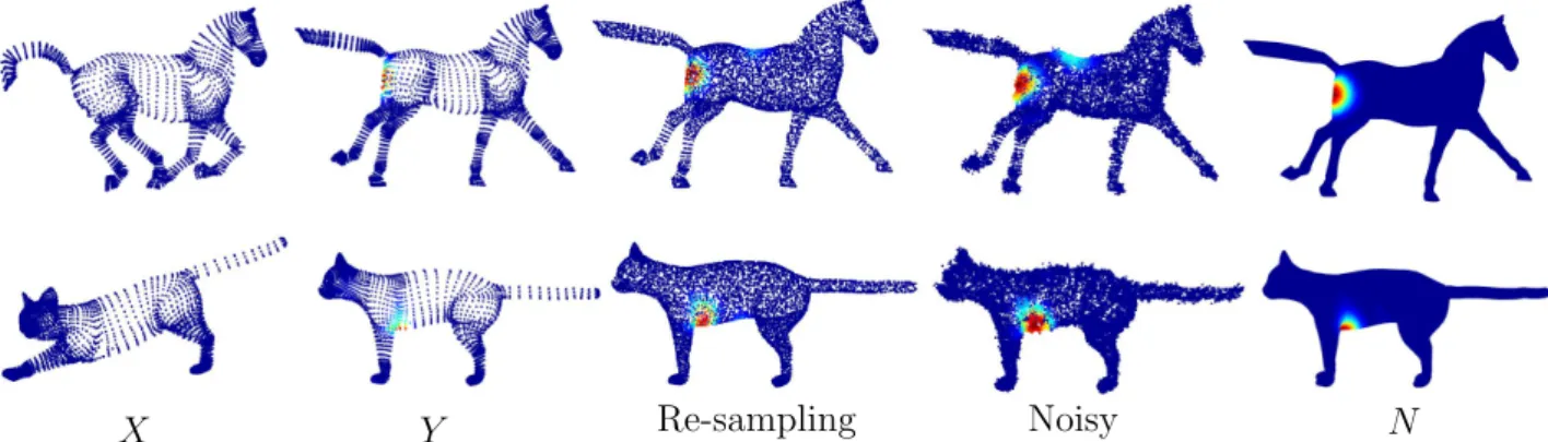
j ˜ KX(i, j) else WX←− − ˜KX(i, j).Using these constructions, we observe that the robustness is evi-denced in the results from our PCD setting as well. In Figure10, we tested with point clouds sampled from horses (8431 points) and cats (7207 points). Point clouds X ,Y come from two meshes in point-to-point correspondence, the highlighted functions on Y are shown to be consistent with the ones computed in the mesh setting on N (see the right-most column). We then resampled point clouds on shape Y while keeping the total number of points unchanged, and computed the highlighted function with respect to X and the resam-pled point cloud. At the end, a further step was taken to add noisy points on the resampled point clouds. Given a point cloud, we first randomly select nppoints from it. Then for a selected point p, we perturb p = (px, py, pz) ∈ R3to (px+ dx, py+ dy, pz+ dz) where dx, dy, dz are one-dimension random variables distributed normally with mean 0, and standard deviation ¯d , which is the median of the distances from a point to its nearest neighbor. Repeating the
displacements r times for each selected point, we enlarge the origi-nal point cloud with nprmore points. The stability of (area-based) shape difference operator is again verified by the consistency of areas highlighted by the functions.
On the other hand, we have seen in Figure4that although the eigenfunctions of the graph Laplacian on the point cloud are dis-tinct from those of the LBO on the mesh, the eigenfunctions of the shape difference operators are comparable. We further explore this by considering the pair of cats taken from the bottom row of Figure10. In particular, we computed the eigenfunctions of the LBO on mesh N and of the graph Laplacian on Y and the per-turbed resampled point cloud. The highlighted functions and part of the eigenfunctions with respect to the three representations are depicted in Figure11. Again, changing the representation of the shape causes significant perturbations on the eigenfunctions, how-ever, as illustrated in Figure10, the areas indicated by the respective highlighted functions remain similar to each other.
6.4. Analyzing Shape Collections
The experiment above shows the stability of the shape difference operators for analyzing maps between a single pair of shapes in a multi-scale way. As we prove in Section4, the shape difference op-erators are stable with respect to perturbations on the input shapes. To demonstrate this, we repeat one of the experiments in [?] (see Figure 3 on page 7 therein), but in the point cloud setting. We com-pute the shape difference operators and then vectorize them so that we can apply PCA. The PCA embeddings in R2are depicted in the right two columns of Figure12.
The top row of Figure 12depicts the embeddings for the de-formed spheres. Both layouts uncover the grid structure of the orig-inal shape collection. The results in [?] suggest that in both area and conformal cases, the variances of the first two principal components are evenly close to 50 percents. In our results: (1) Area-based case: though the sum of percentages add up to almost 100, the grid is unbalanced and stretched along the direction of the first principal component; (2) Conformal case: balance preserved, the shapes of the first and the second rows are not well differentiated, suggesting that the operators are less sensitive to small changes.
The bottom row shows the layouts for the galloping horse se-quence, which consists of two cycles of continuous movement of the horse. Our results successfully capture the circular structure of the sequence, as depicted in the layout. The plot also reveals the fact that there are more conformal distortions than area distortions in this data, as the range of layout in the third column is larger than that in the second one.
Overall, we conclude from these experiments that although the results from the PCD setting are not always as accurate as those from the mesh setting, our results capture most of the basic and significant information hidden in the data. Considering that we start from a much coarser understanding of the input shapes , these re-sults are non-trivial and quite remarkable, especially given the well-known instability in the eigenfunctions of the LBO.
Re-sampling
Noisy
Y
X
N
Figure 10: Robustness of results from the PCD setting: X and Y are the original point clouds extracted from meshes. In the third column, we resampled point clouds on the polygonal mesh, and then we added noisy point displacements to that in the forth column, which are both generated with np= 400, r = 20, i.e. there are 8000 more noisy points (see the text for details). All the area-based highlighted functions are computed at scale k= 50. On the rightmost column are the highlighted functions from the mesh setting.
Highlighted Function
Figure 11: Left: the highlighted functions on the mesh (top), the noiseless point cloud (middle) and the noisy point cloud (bottom). The 11th to the15theigenfunctions of the LBO on mesh (top), the graph Laplacian constructed on top of the original point cloud (middle) and of the resampled noisy point cloud (bottom).
7. Conclusion and Future Work
In this paper we present two types of stability guarantees for the shape difference operators. We also introduce a new multi-scale scheme for extracting information from the shape difference oper-ators, which is provably stable in contrast to the original one pro-posed in [?]. From a practical point of view, we present a pipeline for constructing shape difference operators on point clouds, which extends the range of applications of the related frameworks.
Several follow-up problems arise along our investigation. We especially remark the optimization problem attached to our new multi-scale scheme. As the new scheme provides more stable re-sults in theory, it is appealing to design an efficient implementa-tion. It is as well appealing to consider more rigorous analysis of our pipeline for point cloud data.
Acknowledgement The authors would like to acknowledge the ANR TopData (ANR project TopData ANR-13-BS01-0008), the ERC Gudhi project (Geometric Understanding in Higher Dimen-sions), Marie-Curie CIG-334283, a CNRS chaire d’excellence,
chaire Jean Marjoulet from Ecole Polytechnique, FUI project TAN-DEM 2, a grant from the Direction Générale de l’Armement (DGA) and a Google Focused Research Award.
References Appendix A:
Here we outline the proofs for the main theorems in this paper. We refer interested readers to the corresponding supplemental material for detailed proofs.
Theorem4.1 and Theorem 4.2: First we can prove L2(N) = L2( ˜N) with proposition3.2. To verify the convergence, we first prove that R
Nf V f dνN−RNf ˜V f dνN vanishes as aM, aN, bM, bN converge to 1 simultaneously. Then due to the fact that V is self-adjoint, we prove R
NgV f dνN− R
Ng ˜V f dνN vanishes under the same condition. Lastly, we let g = V f − ˜V fand finish the proof.
The idea of proving in the case of conformal shape differ-ence operator is analogous to the area-based one, but proving
PCA layout for the area-based Shapes in dataset, indexed left
to right and top to bottom shape difference operators.
PCA layout for the conformal shape difference operators. Figure 12: PCA plot of the two shape difference operators.
R
Nh∇ f , ∇R f igNdνN− R
Nh∇ f , ∇ ˜R figNdνN→ 0 is slightly more
complicated as both the measure and the inner-product are per-turbed.
Theorem5.1and Theorem5.3: Given parameters C0> C, our strategy is to find for any function w ∈ A(C0) a function ¯w∈ A(C), such that |E(w) − E( ¯w)| is upper-bounded by some variable with respect to C0− C, which vanishes as C0→ C. Regarding the con-formal case, we apply the same idea, i.e., find for any function w∈ Acon f(C0) a function ¯w∈ Acon f(C), such that |F(w) − F( ¯w)| is uniformly bounded by a variable depending on C0−C.
Theorem5.2: The key observations to proving this theorem are: first, A(C) and ˜A(C) are interleaving, i.e., for any C > 0 we can find a C0 such that A(C) ⊂ A(C0) and vice versa; second, given a w∈ L2(N) = L2( ˜N), the ratio of E(w) to ˜E(w) is two-side bounded with respect to aM, bM, aN and bN. The theorem is obvious then after verifying those observations.
![Figure 1: (a) Given two shapes M,N and a map T between them, the functional operator V is generated as one of the shape difference operators introduced in [?]](https://thumb-eu.123doks.com/thumbv2/123doknet/13402390.406401/2.892.127.778.313.560/figure-given-functional-operator-generated-difference-operators-introduced.webp)