Clustering in Dynamic Causal Networks as a Measure of Systemic Risk on the Euro Zone

(1)

HAL Id: halshs-01339826

https://halshs.archives-ouvertes.fr/halshs-01339826v2

Submitted on 7 Dec 2016

HAL is a multi-disciplinary open access

archive for the deposit and dissemination of

sci-entific research documents, whether they are

pub-lished or not. The documents may come from

teaching and research institutions in France or

L’archive ouverte pluridisciplinaire HAL, est

destinée au dépôt et à la diffusion de documents

scientifiques de niveau recherche, publiés ou non,

émanant des établissements d’enseignement et de

recherche français ou étrangers, des laboratoires

Clustering in Dynamic Causal Networks as a Measure of

Systemic Risk on the Euro Zone

Monica Billio, Lorenzo Frattarolo, Hayette Gatfaoui, Philippe de Peretti

To cite this version:

Monica Billio, Lorenzo Frattarolo, Hayette Gatfaoui, Philippe de Peretti. Clustering in Dynamic

Causal Networks as a Measure of Systemic Risk on the Euro Zone. 2016. �halshs-01339826v2�

(2)

Documents de Travail du

Centre d’Economie de la Sorbonne

Clustering in Dynamic Causal Networks as a

Measure of Systemic Risk on the Euro Zone

Monica B

ILLIO,

Lorenzo F

RATTAROLO,

Hayette G

ATFAOUI,

Philippe D

e

P

ERETTI

2016.46R

(3)

Clustering in Dynamic Causal Networks as a

Measure of Systemic Risk on the Euro Zone

Monica Billio, Lorenzo Frattarollo

y

_{, Hayette Gatfaoui,}

z

_{, Philippe de Peretti}

x

September 27, 2016

Abstract

In this paper, we analyze the dynamic relationships between ten stock exchanges of the euro zone using Granger causal networks. Considering returns for which we allow the variance to follow a Markov-Switching GARCH or a Changing-Point GARCH process, we …rst show that over di¤erent periods, the topology of the network is highly unstable. In partic-ular dynamic relationships vanish over very recent years. Then, expanding on this idea, we analyze patterns of information transmission within the network. Using rolling windows to study networks’ topology in terms of information clustering, we …nd that the nodes’state changes continually. Moreover, the system exhibits periods of ‡ickering in information trans-mission. During these periods of ‡ickering, the system also exhibits desyn-chronization in the information transmission process. These periods do precede tipping points or phase transitions on the market, especially before the global …nancial crisis, and can thus be used as early warnings. To our knowledge, this is the …rst time that ‡ickering in information transmission

Department of Economics, University Ca’Foscari of Venice, Fondamenta San Giobbe 873, 30121, Venice, Italy.

y_{Department of Economics, University Ca’Foscari of Venice, Fondamenta San Giobbe 873,}

30121, Venice, Italy.

z_{IESEG School of Management (LEM-CNRS) and Labex ReFi, Socle de la Grande Arche,}

1 Parvis de la Défense, 92044 Paris La Défense and Centre d’Economie de la Sorbonne, University Paris 1 Panthéon-Sorbonne, gatfaoui@univ-paris1.fr, h.gatfaoui@ieseg.fr.

x_{Corresponding author, Centre d’Economie de la Sorbonne, University Paris 1}

Panthéon-Sorbonne, 106-112 Boulevard de l’Hôpital, 75013 Paris. Tel: 00 33 1 44 07 87 63, peretti@univ-paris1.fr.

(4)

is identi…ed on …nancial markets, and that ‡ickering is related to phase transitions.

Keywords: Causal Networks ; Topology ; Flickering ; Desynchronisa-tion ; Phase TransiDesynchronisa-tions.

JEL codes: C1, C4, G1.

1 Introduction

Consider an electronic component designed to emit a signal which is about to fail, that is about to switch from one state to an other. This component is likely to start emitting abnormal signals, or signals in an abnormal way before the failure, rather than abruptly failing. For instance, we are likely to observe a ‡ickering signal before a phase transition occurs. Consider further the compo-nent as part of an electronic device, which is connected to other compocompo-nents, forming then a complex interdependent dynamic system. Two questions then arise: i) What will be the impact of the component’s failure on the whole sys-tem? In other words, will the electronic device fail because of the failure of one component ? and ii) Is it possible to know in advance that a failure will occur ? One way to answer the …rst question is to look at the integrated circuit of the device (i.e. the topology) and to focus on the importance of the component in terms of centrality and/or the number of components connected to it (i.e. the degree). To answer the second question, one …rst needs to recover the topology of the system, and next to look at the information di¤usion processes (i.e. the signals) so as to identify abnormal periods prior to the failure at the individual and/or the macro level (i.e. component versus circuit level).

Turning to …nancial systems and systemic risk, the …rst question has been adressed by a number of authors using networks. Relating systemic risk to the concepts of connectedness, contagion, and therefore di¤usion of exogenous and/or endogenous shocks within and/or across …nancial sectors (see Bisias et al. 2012), Allen and Gale (2000) as well as Acemoglu et al. (2013) show that highly interconnected networks are more resilient to small shocks but not to large ones. Battiston et al. (2013) focus on the frailty of nodes, and then study cascading e¤ects as Motter and Lai (2002) do. In such models, the focus is set on the impact of the failure of one or several nodes on the whole system.

(5)

Furthermore, Hackett et al. (2011) and Payne et al. (2009) emphasize the importance of networks’topology while studying clustered and degree-correlated networks respectively.

Our paper clearly relates to the second question, that is on early warning indicators prior to a phase transition (i.e. non-crisis versus crisis periods). We consider …nancial systems as being possibly critically self-organized (Bak et al., 1987, Bianconi and Marsili, 2004). In particular, local interrelations between the system’s components build up a coordinated system or network. Such self-organised network/system will turn into a critical behavior (i.e. tipping point and phase transition) without the e¤ect of external forces or drivers. In this light, our main contribution is to provide early warnings of phase transitions for the whole system (or network), which is highly suggestive of systemic risk. To detect early warnings, we adopt a two-step methodology. First, we recover the network topology using non-causality tests as suggested in Billio and al. (2012). Nevertheless, we use a di¤erent class of Granger non-causality tests, within the framework of independence tests for time series1. Such tests are per-formed on normalized innovations of Generalized Auto-Regressive Conditional Heteroskedastic (GARCH) models in which we allow the variance processes to have recurrent (Markov-Switching GARCH) or non-recurrent states or regimes (Changing-Point GARCH). To model series, we adopt the Bayesian Bauwens et al. (2014) methodology. Independence tests for time series are very versa-tile and provide a very rich information concerning instantaneous correlations, non-causality over a given number of lags, or at a given lag. They thus allow for capturing the complex interplay such as feedbacks and spillover e¤ects, and are used to build directed and undirected, as well as weighted and binary net-works here. Despite its apparent simplicity, it has been suggested by Zhou et al. (2014) in integrate-and-…re neuronal systems (see also Winterhalder et al., 2005) that Granger non-causality can capture non-linear relationships.

Once the topology is recovered, we …rst propose a period-speci…c analysis of the contagion process within the network while discriminating between crisis and non-crisis periods. We mainly show that the nodes’ states are highly

un-1_{See Hong (1996), Duchesne and Roy (2001), Koch and Yang (1986), El Himdi and Roy}

(6)

stable over time. Expanding on this idea, we identify phase transitions based on the very short-term dynamic di¤usion process of information/shocks accross nodes. Such nodes’ short-term di¤usion processes are interpreted as signals. Our dynamic signal analysis relies on a six-month rolling window, and focuses on triangular clustering patterns or motifs of information di¤usion as de…ned by Faggiolo (2007), including spillover and feedback e¤ects.

Considering daily data about ten main European stock indices form 1994 to 2014, our …ndings are manyfold: i) With respect to period-speci…c analysis, correlations prevail over the data sample and are regime-dependent. Such corre-lations increase up to the period following the crisis, and then start decreasing, ii) Besides, the number of causal relationships as well as their strength increases up to the crisis period but vanishes after the crisis period. Over the remain-ing sample history, there exist very few and very weak causal relationships, iii) Based on a rolling window analysis, we …rst show that periods of clustering precede periods of ‡ickering in clustering, which are followed by a tipping point and a phase transition. The phase transition begins with an abrupt clustering phenomenon for all stock exchanges. Such sudden phenomenon indicates a si-multaneous phase transition of all stock markets (i.e. synchronized clusters). Interestingly, ‡ickering periods also highlight times when stock exchanges ex-hibit desynchronized information ‡ow processes. In particular, Euro zone stock exchanges exhibit clusters’desynchronization approximately one year before the Global Financial Crisis. At last, the end-of-crisis period exhibits an exceptional and speci…c clustering phenomenon, which is followed by the sudden disappear-ance of clusters. Hence European stock exchanges seem to stop interacting together. To our knowledge, we are the …rst to study clustering, or equiva-lently, information di¤usion patterns within causal networks. Clearly, ‡ickering in clustering as well as desynchronization in information transmission patterns could serve as early warnings indicators of phase transition on the market.

This paper is structured as follows. Section 2 introduces the econometric methodology. Section 3 focuses on the statistical properties of the data and applies the Bauwens et al. (2014) methodology. Section 4 implements period-speci…c independence and non-causality tests on …ltered and orthogonalized data. Section 5 focuses on early warning indicators of crisis. Finally, Section 6

(7)

concludes.

2 Econometric methodology

Let r = f(r(1)t 0; r (2)0 t ; :::; r (N )0

t )0; t 2 Zg be a set of N log-returns of a main index

of a stock-exchange, observed over T periods. Assume that each component of r admits a Generalized Auto-Regressive Conditional Heteroskedastic process (GARCH) representation (Bollerslev, 1986):

r(i)_t p P l=1 (i) l r (i) t l c (i) ₌ q_h(i) t (i) t (1) (i) t = q h(i)t (i) t (2)

h(i)_t = !(i)+ (i) (i)2_{t 1}+ (i)h(i)_{t 1} (3)

(i)

t iid(0; 1) (4)

Moreover, as T becomes large, consider that returns might also exhibit breaks in their volatility process. Then, de…ne a more realistic Data Generating Process (DGP) as: r(i)_t p P l=1 (i) l r (i) t l c (i) ₌ q_h(i) t (i) t (5) (i) t = q h(i)_t (i)_t (6) h(i)t = !(i)st + (i) st (i)2 t 1+ (i) sth (i) t 1 (7) (i) t iid(0; 1) (8)

Equation (7) allows the parameters in the variance equation to switch from one value to another. We focus on two kinds of switching processes: i) Switch-ing processes with recurrent states, i.e. Markov-SwitchSwitch-ing (MS-) GARCH (see Francq and Zakoian, 2008), ii) Switching processes with non-recurrent states, i.e. Change-Point (CP-) GARCH (He and Maheu, 2010). Let ST = fs1; s2; :::; sTg0,

the latent process fstg is a …rst-order Markovian process with transition matrix

(8)

PS = 0 B B B B B B B B B @ p11 p12 p13 p1K 1 PK_j=1p1j p21 p22 p23 p2K 1 PK_j=1p2j pK1 pK2 pK3 pKK 1 PKj=1pKj pK+1;1 pK+1;2 pK+1;3 pK+1;K 1 PKj=1pK+1j 1 C C C C C C C C C A ; where pij = P [st= jjst 1= i]; or by: PC= 0 B B B B B B B B B @ p11 1 p11 0 0 0 0 p22 1 p22 0 0 0 0 0 pKK 1 pKK 0 0 0 0 1 1 C C C C C C C C C A :

where PScorresponds to a Markov switching process with K +1 regimes, and

PCdescribes a change-point process with K breaks. Then, de…ne the estimated

normalized return_b(i)_t = (bh(i)_t ) 1=2_b(i)

t , i = 1; 2; :::; N:

Next, we build binary and weighted undirected networks (BUN, WUN) as well as binary and weighted directed networks (BDN, WDN). A binary network is described by a graph G = (N; A), where N is the number of nodes, here the number of stocks, and A = faijg is the N N adjacency matrix. For binary

networks, nodes i and j are connected by an edge if aij = 1. For a graph

G = (N; A), de…ne the indegree, outdegree and total degree for node i as: din_i = X j6=i aji= (A0)i1 (9) dout_i = X j6=i aij= (A)i1 (10) dtot_i = din_i + dout_i = (A0+ A)i1 (11)

where A0 _{is the transpose of A:}

Also of interest are the bilateral edges between i and j, i.e. aij = 1 and

aji= 1:

d$_i =X

j6=i

aijaji= A2ii (12)

The weighted networks parallel the binary one. They are de…ned by the graph G = (N; W) where W = fwijg is a matrix of weights ranging from 0 to 1.

(9)

Then, replacing in (9) to (11) A by W one can focus on the strength of a node, and the strength of the net.

To build BUN, WUN, BDN and WDN, i.e. to recover the topology of the network, we use non-correlation, or independence tests for time series. These tests are very versatile and are based on normalized residuals cross-correlations of models (1) or (5). They encompass several tests: i) Non-signi…cance of a cross-correlation at a lag k = 0 or k 2 f1; Mg, ii) Portmanteau test to check for overall independence, i.e. non-signi…cance of all leads and lags, iii) Portmanteau tests to check for non-causality in the Granger sense. Independence tests for time series have been introduced by Haugh (1976). They have been extended by Hong (1996), Duchesne and Roy (2003) or Koch and Yang (1986), this latter also taking into account patterns in cross-correlations. El Himdi and Roy (1997), Pham et al. (2001) or Hallin and Saidi (2001) among other present multivariate extensions. Also, El Himdi et al. (2003) propose a nonparametric test. In this paper we have used the El Himdi and Roy (1997), Hallin and Saidi (2001) and El Himdi et al. (2003) approaches, as well as several re…nements2. Having obtained very similar results, in the sequel, only the ones based on the El Himdi and Roy (1997) methodology are presented.

Generally, let _b(1) _{= fb}(1)_t _{; t 2 Zg and b}(2) _{= fb}(2)_t _{; t 2 Zg be two sets of} …ltered series using univariate or multivariate models, i.e. (normalized) residuals of models estimated independently with values in Rd1 _{and R}d2_{. De…ne the}

covariances and cross-covariances C(hh)_b (0) and C(12)_b (k) as:

C(hh)_b (0) = T 1 T X i=1 b(h)t b (h)0 t ; h = 1; 2 (13) C(12)_b (k) = 8 < : T 1PT i=1b (1) t b (2)0 t k 0 k T 1 T 1PT i=1b (1) t b (2)0 t k 1 T k 0: (14) the correlations and cross-correlations are de…ned as:

R(hh)_b _{(0) = fdiag C}(hh)_b _(0)g 1=2C(hh)_b _{(0)fdiag C}(hh)_b _(0)g 1=2 (15) and:

R(12)_b _{(k) = fdiag C}(11)_b _(0)g 1=2C(12)_b _{(k)fdiag C}(22)_b _(0)g 1=2 (16)

2_{In particular, instead of cross correlations, we have also used partial cross-correlations}

(10)

Then the null of non-correlation or independence can be tested using the port-manteau statistic: QM = T M P k= M T T _jkj vec R (12) b (k) 0 R(22)_b (0) R(11)_b (0) 1 vec R(12)_b (k) (17) Under the null of non-signi…cance of cross correlations at all leads and lags, QM

is distributed as a Chi-square with (2M + 1)d1d2 degrees of freedom.

Using the above statistic,Granger non-causality tests are easy to derive by summing over f1; Mg or f M; 1g. For instance, testing for Granger non-causality from X(2) _{to X}(1) _(X(2) _{; X}(1)_{) amounts to computing the test}

statistic: Q+_M = T M P k=1 T T k vec R (12) b (k) 0 R(22)_b (0) R(11)_b (0) 1 vec R(12)_b (k) (18) Similarly, to test for non-causality from X(1) _{to X}(2) _(X(1) _{; X}(2)_{), one is to}

use: Q_M = T M P k= 1 T T _jkj vec R (12) b (k) 0 R(22)_b (0) R(11)_b (0) 1 vec R(12)_b (k) (19) Under the null, both tests (18) and (19) are chi-square distributed with M d1d2 degrees of freedom.

All above tests are portmanteau tests. It is also useful to look at the signif-icance of an individual lead/lag. A natural test statistic is given by:

Q(k) = T T T _jkj vec R (12) b" (k) 0 R(22)_b_" (0) R(11)_b_" (0) 1 vec R(12)_b_" (k) (20) which is also chi-square distributed with d1d2 degrees of freedom.

In this paper, to build BUN and WUN we use (17) with k = 0 and M = 7 and (20) with k = 0. Therefore, an edge exists between two nodes, if the test is rejected at the 5% threshold. For BDN and WDN we use (18), (19) and (20) with k 6= 0; M = 7 (and M = 1 for 20), and this for each pair of the set b.

3 Data properties and orthogonalization

Table (1) displays benchmark stock market indices as well as related ARCH-LM test statistics for the ten European countries under consideration as well

(11)

as U.S.A. (SP500 index return). The analysis is based on daily data spanning January 1998 to May 2014. Except for one return series, all series exhibit non-null skewness and excess kurtosis. Moreover, as expected, all series exhibit second-order dependence.

Please insert Table (1) about here

To test for breaks in volatility processes, and discriminate between recurrent (MS-GARCH) and non-recurrent (CP-GARCH) regimes, we follow Bauwens et al. (2014). The methodology on a Bayesian approach which combines sequential Monte Carlo (SMC) and Markov Chain Monte Carlo (MCMC) methods. For each model, we perform 10,000 particle Gibbs iterations. After convergence in the Geweke sense (Geweke, 1992), we then compute the marginal likelihood by bridge sampling (1,000 iterations). The number of particles is set to 150 for changing point models, and 250 for Markov Switching models. Finally, we select the model for which the marginal likelihood is maximal.

Please, insert Table (2) about here

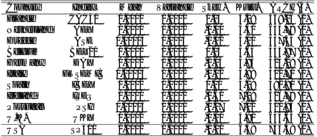
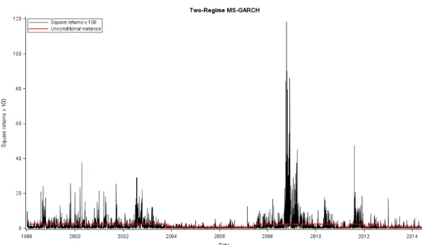
Table (2) displays the results of the Bauwens et al. (2014) Bayesian pro-cedure. Results support a no-break model for AEX and a two-break model (i.e. three non-recurrent states) for ASE. All other series exhibit a recurrent two-state Markov-Switching process (i.e. high and low volatility regimes). In the sequel, normalized residuals will be based on these models. With regard to SP500, our results are similar to Bauwens et al. (2014), as shown by Figure (1).

Please insert Figure (1) about here

Using the above procedure, we build two sets of normalized residuals b = fb(1)t 0;b (2)0 t ; :::;b (10)0 t ; t 2 Zg =f((bh (1) t ) 1=2b (1) t )0; ((bh (2) t ) 1=2b (2) t )0; :::; ((bh (10) t ) 1=2b (10) t )0; t 2

Zg corresponding to European stock exchanges, and bBench = fb(11)t 0; t 2

Zg =f((bh(11)t ) 1=2b (11)

t )0; t 2 Zg corresponding to the SP500. Once data are

…ltered by the proper Data Generating Process, we further need to adress a key issue. To build networks, we use non-correlation and non-causality tests between each pair of nodes, i.e. between each pairs of _{b. Nevertheless, it is} well known that in bivariate systems, non-causality and non-correlation tests

(12)

might be biased due to the omitted variable problem (i.e. spurious relation-ships, see e.g. Triacca, 1998). To tackle this issue, we consider the SP500 index as a central variable which in‡uences all European exchanges. We then adopt the Duchesne and Nkwimi (2013) methodology to orthogonalize series with re-spect to the causal structure of another series. The orthogonalization method is a two-step procedure. First, we compute the cross-correlations between each component of _{b and b}Bench_{. For each k 2 f0; :::; Mg, we compute the test} statistics (20) and keep the signi…cant lags. Then, we regress fb(i)t gTt=1 on the

signi…cant lags of fb(bench)t gTt=1,and keep the corresponding residuals fb" (i)

t gTt=1.

Doing this for each European stock index i = 1; 2; :::; N , we build a set of N = 10 orthogonalized series _{b" = f(b"}(1)0_t ;_b"(2)0_t ; :::;_b"(N )0_t )0_{; t 2 Zg with regard to SP500}

index. In the sequel, all tests are implemented on this set.

4 Period-based analysis

We …rst perform our analysis over 6 di¤erent periods given by Table (3). As mentioned above, three kinds of networks can be built: i) Networks where nodes are connected if the null of independence is rejected at 5%, ii) Networks where nodes are connected if non-causality is rejected at 5%, also called functional connectivity, iii) Networks where nodes are connected if for a given lead/lag the null of non-signi…cance of the individual cross-correlation is rejected.

Please insert Table (3) about here

Results are summarized by both heatmaps and networks. To build heatmaps, we use both total degrees (11) and weights. To compute weights ranging from 0 to 1 for a single node, and as all tests of connectivity are based on sums of individual (squared) cross-correlations or on individual cross-correlations at a given lag, we proceed as follows. For independence and non-causality tests and for each period, we divide the test statistics by the maximal value obtained over one period. For individual lags, we just take the absolute value of the cross-correlations.

(13)

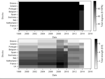
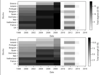
Figure (2) displays the heatmaps resulting from independence tests for K = 7. Focusing on degrees (upper panel), all stock exchanges are highly intercon-nected over the …rst 5 periods whereas, over the last period, Greece disconnects from the network of Euro zone stock exchanges. Moreover, the total degree slightly decreases (i.e. less interconnections) for all stock markets except for Ireland and Portugal. As regards strength (lower panel), which ranges from 0 to 9, the main striking feature is the abrupt change in the strength of depen-dence among stock exchanges after the post-crisis period. During the crisis, the strength of the network increases, remains high during the post-crisis period, and then seems to vanish. As a result, the closer we get to the crisis period, the more mutually dependent stock exchanges become, due to the increasing strength of their network. All stock exchanges being connected during the cri-sis, connections’ strength reaches their highest level by that time. However, some stock exchanges start disconnecting after the crisis period. Furthermore, Greece exhibits a weak connection to the Euro zone network of stock exchanges. Thus, even if the Greek stock exchange is risky, its has a reduced impact on other Euro zone stock exchanges.

Figures (3) and (4) provide a deeper analysis of the Euro zone network of stock exchanges while focusing solely on either non-correlation or non-causality tests. Focusing on non-correlation tests, Figure (3) provides a similar informa-tion as previous heatmaps because Euro zone stock exchanges are highly cor-related. Speci…cally, all stock exchanges are strongly interrelated, and strength begins to increase before the Global Financial Crisis, being maximal during and just after the Global Financial Crisis. Such clustering phenomenon emphasizes the strong simultaneous and joint reaction of stock exchanges. However, there is an abrupt downturn in the network’s strength after the post-crisis period so that some stock exchanges start disconnecting.

As regards non-causality tests (K = 7), Figure (4) provides key informations about both the reception (i.e. incoming information) and transmission (i.e. outgoing information) of …nancial shocks across stock market places. Before the Global Financial Crisis, the degrees of the network are quite high up to the crisis period, and then vanish. A similar result appears when one focuses on the strength of the network. Strikingly at the end of sample (over period

(14)

6) only three stock exchanges are weakly interconnected from a causal point of view. Such feature suggests the absence of dynamic interrelations over the recent periods, and thus a low risk of contagion (i.e. almost non-existing spillover and no feedback e¤ects).

Please insert here Figures (3) and (4)

The network representations corresponding to heatmaps in Figure (4) are illustrated by Figures (5), (6) and (7). Corresponding network representations are provided for the six periods covering the data sample (see Table 3). Such …gures emphasize the evolution of the dynamic causal network of Euro zone stock exchanges over time. Speci…cally, the network’s density increases up to the crisis period, diminishes during the post-crisis period, starts increasing during the sovereign debt crisis period, and then strongly drops over the post-sovereign debt crisis period. Over the last period of the sample, there are very few causal relationships between Euro zone stock exchanges. Moreover, previous …gures display incoming and outgoing connections between the network’s nodes (i.e. between stock exchanges). Thus, we observe clearly the directional propagation of shocks across stock market places over time.

Please insert here Figures (5), (6) and (7)

5 Flickering in information transmission

One major result of the previous section is that the topology of the network changes from one period to another. Speci…cally, information transmission chan-nels within the network are unstable over time, which leads to complex patterns of transmitted and emitted signals. It is therefore of interest to focus on such an unstability in order to: i) Check if the evolution of certain patterns of infor-mation transmission match with the di¤erent phases of the …nancial market as reported in Table (3), ii) Determine early warning indicators, preceding tipping points or phase transitions.

(15)

We use a six-month rolling window, and focus on the very short-term (K 1) information di¤usion schemes, and in particular, on speci…c triangular patterns or motifs as de…ned by Faggiolo (2007). Table (4) introduces the de…nitions for four types of clustering coe¢ cients (C_ij; j = Cyc; Out; M id; In) as well as the total clustering coe¤cient (C_iD) for BDNs and WDNs. For a node i, the cycle pattern (Cyc) corresponds to feedback e¤ects and the out pattern (Out) to spillovers. In the middleman pattern (M id), the node i appears to be a relay in the information propagation (i.e. intermediate transmitter). In the in pattern (In) , the node receives information from its neighbors (i.e. receiver). Thus, all complex interactions are well captured by the various clustering coe¢ cients under consideration.

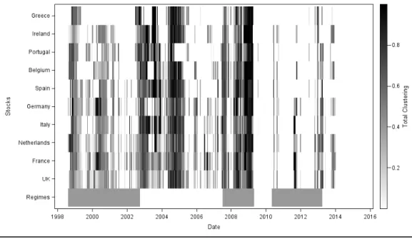
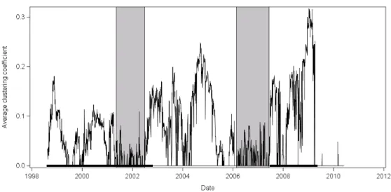
Results are displayed in Figures (8), (10) and (11). Figure (8) plots the heatmap of total clustering for BDNs (upper panel), ranging from 0 to 1. This Figure also displays an indicator of crisis (grey) and non crisis (white) peri-ods as mentionned in Table (3). Such indicator is labelled ’Regimes’. For a comparison purpose, we also plot the time-path of the density of the network (lower panel). Figure (10) plots heatmaps for each kind of triangular patterns for BDNs. At last, we average the total clustering coe¢ cients of WDNs over each rolling window (see Figure 11).

Interpreting clustering in dynamic networks as emitted or received signals, allows to study the whole dynamics of the system. The heatmap of total clus-tering (Figure 8) unveils key information. Starting from the Dot.com bubble, each return series, except for Greece, does exhibit very large periods of clus-tering with variable intensities. Then, around March 2001, clusclus-tering abruptly stops, and the system turns into a ‡ickering period so that some nodes alter-nate between clustering and non-clustering states. During such periods, each node ‡ickers between being in and out the information di¤usion process. At the same time, periods of clustering become shorter. In other words, the net-work’s nodes continually become active or inactive, emphasizing that we face an ever-changing network (Odum and Barret, 2005) in terms of information trans-mission. This rapid alternation of states does precede a phase transition, the market entering then the pre-crisis period. The beginning of the transition is characterized by a sudden rise of clustering for all stock exchanges at nearly the

(16)

same time. Focusing on the pre-crisis period, similar patterns are found. From the beginning of the pre-crisis period to early 2005, the whole system exhibits a high degree of clustering, especially after 2004. Then, abruptly in early 2005, the system starts to ‡icker, alternating between clustering and non-clustering states. Such feature is also re‡ected in the density of the network in early 2006, and more speci…cally in the average clustering coe¢ cient (Figure 11). Hence, compared to Billio et al. (2012), the relevant information, may not be the in-crease in degrees before a …nancial crisis, but rather the ‡ickering in degrees, which occurs after their increase (e.g. during the pre-crisis period).

Focusing on the Global Financial Crisis period, it is interesting to notice that it begins with an abrupt change in clustering (phase transition) for the whole system, and also ends with an abrupt change. Over the post crisis period, clustering totaly disappears, which is line with our previous causality tests. Anecdotal results show that the sovereign debt crisis period begins and ends with a sudden rise in clustering. As a consequence, our methodology’s added-values are twofold. First, we are able to detect forthcoming phase transitions, and second, we are able to date crises’ beginnings and ends. Such dating matches with the di¤erent market phases reported in Table (3). Therefore ‡ickering precedes a phase transition and acts as an early warning.

Flickering phenomena as early warning signals have been reported in complex systems, especially in ecology (e.g. Dakos et al., 2013) as well as in climatology (Livina et al., 2010). Interestingly, Dakos et al. (2013) noticed that ‡ickering between basins of attraction may appear far before bifurcation or tipping points, and could then be used as early warnings. To our knowledge, this is the …rst time that ‡ickering in information di¤usion processes is studied, exhibited and described in …nancial systems.

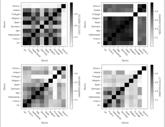
In addition to rapid ‡ickering, before a tipping point occurs, the informa-tion di¤usion process starts desynchronizing accross nodes. We observe either asynchonicity of signals or arising noises within the system. To handle such pattern, we compute a dummy variable taking a unit value if the node enters total clustering, and 0 otherwise. Then, we divide the pre-crisis period into four equal sub-samples, and compute the Jaccard similarity coe¢ cient over each sub-sample to capture the transition from synchronicity to asynchronicity. The

(17)

Jaccard similarity coe¢ cient is a pairwise correlation index which checks for the similarity in the date of appearance of clusters. Corresponding results are displayed in Figure (12). The darker the color, the more synchronous the nodes become. Synchronization is strong over the two …rst sub-periods (except for Portugal), and then vanishes. Indeed, over the third sub-sample, the network starts desynchronizing. Over the fourth sub-period, there is a disconnection in the information transmission patterns, shown by a decrease of most pairwise correlations. However, the network still exhibits a weak synchronous core, which is composed of Germany, Italy, France and UK. Such feature suggests that, just before the Global Financial Crisis, we have a core network that remains weakly synchronized, and a periphery network, which is fully desynchronized.

Please insert Figure (8) about here

As a conclusion, shocks are continually di¤used and absorbed within the network a long time before the crisis occurs. All the system’s components (i.e. stock exchanges) interact in a synchronous way. Di¤erently, before the crisis, shocks are di¤used and absorbed in a discontinuous and asynchronous manner by network’s components. Information di¤usion patterns become intermittent (i.e. ‡ickering phenomenon), which announces a forthcoming phase transition (i.e. a crisis). The ‡ickering phenomenon appears approximately one year before the crisis. Therefore our results suggest that ‡ickering acts as an early warning signal, and the degree of desynchonization reveals the vicinity of the tipping point.

Please insert Figures (11) (12) (10), and about here

6 Conclusion and discussion

In this paper, we have analyzed the dynamic relationships among ten European stock exchanges. We have focused on networks where two nodes are connected by functional or causal connectivity. Instantaneous correlations are also consid-ered. Our major …ndings are manyfold. Using a period-based analysis, we have found that the network of Euro zone stock exchanges was unstable over time,

(18)

so that the number of connections and their related strength were highly time-varying. Strikingly, there remain very few causal relationships at the end of our data sample (i.e. post-sovereign debt crisis period), indicating that contagion over these recent years seems to be low. Such information is of huge signi…cance to the regulatory authority (e.g. monitoring and marking-to-market processes, assessment of risk exposures, gauging contagion risk). Expanding on the un-stability of the topology, we have focused on motifs of information di¤usion processes (i.e. triangular clusters) in order to capture early warnings of phase transition. We have shown that the whole system exhibited ‡ickering informa-tion clusters with a high degree of desynchronizainforma-tion before a phase transiinforma-tion occurs. As a consequence, ‡ickering in information transmission can act as an early warning signal, and the degree of desynchonization reveals the vicinity of a tipping point. Our analysis, also allows to date crisis periods. To our knowledge, this is the …rst time that ‡ickering in clusters is identi…ed in complex …nancial systems. The ability to extract early warnings about forthcoming crises is use-ful to regulators in order to take preventive measures and mitigate contagion risk. Such tool could e¢ ciently help regulators undertake their monitoring and supervisory activities.

There is an avenue for future research within this area. One would consist in enlarging our dataset to include credit defaults swaps as well as bonds. Another direction could be to study cascading errors, and then relating our network to the riskiness of nodes.

Acknowledgement 1 The research leading to these results has received fund-ing from the European Union Seventh Framework Programme (FP7-SSH/2007-2013) under grant agreement n 320270 SYRTO. This documents re‡ects only the author’s view. The European Union is not liable for any use that may be made of the information contained therein. This work was achieved through the Laboratory of Excellence on Financial Regulation (Labex ReFi) supported by PRES heSam under the reference ANR10LABX0095. It bene…ted from a French government support managed by the National Research Agency (ANR) within the project Investissements d’Avenir Paris Nouveaux Mondes (investments for the future Paris New Worlds) under the reference ANR11IDEX000602.

(19)

References

[1] Acemoglu, D., Ozdaglar, A., and A. Tahbaz-Salehi (2012): Systemic risk and …nancial stability in …nancial networks, NBER Working Paper No. 18727.

[2] Allen, F. and D. Gale (2000), Financial Contagion, Journal of Political Economy 108, 1-33.

[3] Bak, P., Tang, C. and K. Wiesenfeld (1987): Self-organized criticality: An explanation of the 1/f noise, Phys. Rev. Lett. 59, 381-384.

[4] Battiston, S., Bersini, H., Caldarelli, G., Pirotte, H. and T. Roukny (2013) Default Cascades in Complex Networks: Topology and Systemic Risk, Na-ture, Scienti…c Reports 3, Article number: 2759.

[5] Bauwens, L., Dufays, L. and J.V.K. Rombouts (2014): Marginal likeli-hood for Markov-switching and change-point GARCH models, Journal of Econometrics 178, 508-522.

[6] Bianconi, G. and M. Marsili (2004): Clogging and self-organized criticality in complex networks, Phys. Rev. E 70.

[7] Billio, M., Getmansky, M., Lo, A.W. and L. Pelizzon (2012): Econometric measures of connectedness and systemic risk in the …nance and insurance sector, Journal of Financial Economics 104, 535-559.

[8] Bisias, D., Flood, M., Lo, A.W. and S. Valavanis: A survey of systemic risk analytics, O¢ ce of Financial Research, Working paper #0001

[9] Haugh, L.D. (1976): Checking the independence of two covariance-stationary time series: A univariate residual cross-correlation residual ap-proach, Journal of the American Statistical American association 71, 378-385.

[10] Hong, Y. (1996): Testing for independence between two covariance station-ary time series, Biometrika 83, 615-625.

[11] Dakos, V., Van Nes, E.,H. and M. Sche¤er (2013): Flickering as an early warning signal, Theoretical Ecology 6, pp 309-317

(20)

[12] Duchesne, P. and R. Roy (2003): Robust tests of independence between two time series, Statistica Sinica 13, 827-852.

[13] Duchesne, P. and H. Nkwimi (2013): On testing for causality in variance between two multivariate time series, Journal of Statistical Computation and Simulation 83, 2064-2092.

[14] El Himdi, K. and R. Roy (1997): Tests for non-correlation of two multi-variate ARMA time series. Canadian Journal of Statistics 25, 233-256. [15] El Himdi, K., Roy, R. and P. Duchesne (2003): Tests for non-correlation of

two multivariate time series: a nonparametric approach, Research Report CRM-2912.

[16] Faggiolo, G. (2007): Clustering in complex directed networks, Phys. Rev. E 76.

[17] Geweke, J. (1992): Evaluating the accuracy of sampling-based approaches to the calculation of posterior moments, Bayesian Statistics 4, 169-193. [18] Hackett, A., Gleeson, J.-P and S. Melnik (2011): How clustering a¤ects the

bond percolation threshold in complex networks, Physical Review E 83. [19] Hallin, M. and A. Saidi (2005): Testing independence and causality between

multivariate ARMA time series, Journal of Time Series 26, 521-276 [20] Koch, P. and S. Yang (1986): A method for testing the independence

be-tween two time series that accounts for a potential pattern in the cross-correlation function, Journal of the American Statistical Analysis 81, 533-544.

[21] Livina, V. N., Kwasniok, F., and Lenton, T. M., Potential analysis reveals changing number of climate states during the last 60 kyr. Clim. Past 6 (1), 77 (2010).

[22] Motter, A. and Y.-C. Lai (2002): Cascade-based attacks on complex net-works, Physics Review 66, 1-4.

[23] Odum, E. P., and G. W. Barret (2005): Fundamentals of Ecology. Thomson Brooks/Cole, Belmont, California.

(21)

[24] Payne, Joshua, L., Dodds, P.S. and M.J. Eppstein (2009): Information Cascades on Degree-Correlated Random Networks, Physical Review E , 80.

[25] Pham, D.T. and Roy, R and L. Cédras et al. (2003): Tests for non-correlation of two co-integrated ARMA time series, Journal of Time Series Analysis 24, 553-577.

[26] Triacca, U (1998), Non-causality: The role of the omitted variables, Eco-nomics Letters 60, 317-320.

[27] Winterhalder, M., Schelter, B., Hesse, W., Schwab, K., Leistritz, L., Klan, D., Bauer, R., Timmer, J., Witte, H. (2005): Comparison of linear signal processing techniques to infer directed interactions in multivariate neural systems, Signal Process 85, 2137–2160.

[28] Zhou, D., Xiao, Y., Zhang, Y., Xu, Z. and D. Cai (2014): Granger Causal-ity Network Reconstruction of Conductance-Based Integrate-and-Fire Neu-ronal Systems, PLoS ONE 9 doi:10.1371/journal.pone.0087636.

(22)

7 Tables and graphs to be included in the paper

Table 1: Description and statistical properties of index returns Country Index Mean Variance Skew. Kurt. ARCH(4) France CAC40 0.0002 0.0002 0.05 4.29 469.06 (0) Netherland AEX 0.0001 0.0002 -0.10 5.50 634.78 (0) Greece ASE 0.00003 0.0003 -0.02 3.11 337.43 (0) Belgium BEL20 0.0001 0.0001 0.05 5.63 555.97 (0) Germany DAX 0.0002 0.0002 -0.05 3.83 524.29 (0) Italy FTSEMIB 0.00005 0.0002 -0.12 3.88 512.71 (0) Spain IBEX 0.0002 0.0002 0.00 4.19 482.80 (0) Ireland ISEQ 0.0001 0.0002 -0.61 7.19 526.78 (0) Portugal PSI 0.00005 0.0001 -0.27 7.02 301.96 (0) U.K. UKX 0.0002 0.0001 -0.10 5.81 634.65 (0) USA SP500 0.0002 0.0001 -0.20 6.58 745.58 (0)

(23)

Table 2: Marginal likelihoods Regimes 1 2 3 4 5 AEX MS-GARCH -6293.57 -6294.14 -6296.68 AEX CP-GARCH -6293.57 -6298.78 -6297.46 -6302.92 -6307.9 ASE MS-GARCH -7484.95 -7440.39 -7462.49 ASE CP-GARCH -7484.96 -7464.58 -7433.67 -7437.97 -7437.66 BEL20 MS-GARCH -5855.88 -5845.54 -5859.66 BEL20 CP-GARCH -5855.88 -5856.19 -5855.08 -5854.99 -5857.82 CAC40 MS-GARCH -6575.57 -6570.94 -6576.87 CAC40 CP-GARCH -6575.58 -6579.27 -6579.17 -6576.07 -6582.44 DAX MS-GARCH -6672.93 -6671.32 -6680.63 DAX CP-GARCH -6672.93 -6677.58 -6681.49 -6684.95 -6688.8 FTSEMIB MS-GARCH -6587.34 -6579.35 -6587.89 FTSEMIB CP-GARCH -6587.34 -6586.1 -6579.63 -6579.42 -6589.55 IBEX MS-GARCH -6678.06 -6669.91 -6675.54 IBEX CP-GARCH -6678.15 -6679.26 -6673.07 -6675.38 -6681.4 ISEQ MS-GARCH -6155.85 -6141.69 -6157.37 ISEQ CP-GARCH -6155.83 -6155.25 -6155.85 -6145.67 -6156.4 PSI MS-GARCH -5749.94 -5728.98 -5750.49 PSI CP-GARCH -5749.93 -5747.45 -5732.02 -5736.89 -5731.67 UKX MS-GARCH -5692.76 -5691.33 -5698.55 UKX CP-GARCH -5692.75 -5691.44 -5694.12 -5697.48 -5698.27 SP500 MS-GARCH -5775.66 -5765.51 -5776.65 SP500 CP-GARCH -5775.66 -5777.91 -5771.92 -5767.62 -5768.15

Table 3: Periods of the analysis

Name Dates

1 Dot.com bubble 07JAN98-09OCT02 2 Pre-crisis 10OCT02-02JUL07 3 Crisis 03JUL07-01MAY09 4 Post-crisis 02MAY09-30APR10 5 Sovereign debt crisis 01MAY10-31MAR13 6 Post-sovereign debt crisis 01APR13-20MAY14

(24)

Table 4: Patterns of triangles and clustering coe¢ cients (CC) Patterns CCs for BDNs CCs for WDNs Cycle C_iCyc= (A)3ii

din i douti d$i C_iCyc= (W )3ii din i douti d$i Middleman C_iM id= (AA0A)ii din i douti d$i C M id i = (W W0_{W )} ii din i douti d$i In CIn i = (A0_A2₎ ii din i (dini 1) CIn i = (W0_W2₎ ii din i (dini 1) Out COut i = (A2_A0₎ ii dout i (douti 1) C Out i = (W2_W0₎ ii dout i (douti 1) Total C_iD= (A+A0)3ii 2TD i C D i = (W +W0₎3 ii 2TD i Note: TD