HAL Id: hal-02535233
https://hal.archives-ouvertes.fr/hal-02535233
Submitted on 7 Apr 2020
HAL is a multi-disciplinary open access
archive for the deposit and dissemination of
sci-entific research documents, whether they are
pub-lished or not. The documents may come from
teaching and research institutions in France or
abroad, or from public or private research centers.
L’archive ouverte pluridisciplinaire HAL, est
destinée au dépôt et à la diffusion de documents
scientifiques de niveau recherche, publiés ou non,
émanant des établissements d’enseignement et de
recherche français ou étrangers, des laboratoires
publics ou privés.
of the Gironde estuary
Vanessya Laborie, Sophie Ricci, Matthias de Lozzo, Nicole Goutal, Yoann
Audouin, Philippe Sergent
To cite this version:
Vanessya Laborie, Sophie Ricci, Matthias de Lozzo, Nicole Goutal, Yoann Audouin, et al..
Quantify-ing forcQuantify-ing uncertainties in the hydrodynamics of the Gironde estuary. Computational Geosciences,
Springer Verlag, 2019, 24 (1), pp.181-202. �10.1007/s10596-019-09907-7�. �hal-02535233�
(will be inserted by the editor)
Quantifying forcing uncertainties in the hydrodynamics of the
Gironde estuary
Vanessya LABORIE · Sophie RICCI · Matthias DE LOZZO · Nicole GOUTAL · Yoann AUDOUIN · Philippe SERGENT
Received: 2018 07 07 / Accepted: date
Abstract High tide combined with high meteorologi-cal surge levels and discharges in the Garonne and Dor-dogne rivers in the Gironde estuary (south-west France), may lead to high water levels and flooding near the Blayais nuclear power plant and the city of Bordeaux, with significant economic and social impacts. A global sensitivity analysis (GSA) was performed with a Telemac2D numerical model currently used for operational water level forecasts. The major sources of uncertainties were identified by computing the Sobol’ indices for uncer-tain inputs with an analysis of variance (ANOVA) ap-proach for a 7-day storm event in 2003. The generation of the GSA ensemble of simulations consists of sampling scalar and field random variables: constant and uniform friction coefficients, as well as time-varying hydrologi-cal and maritime forcings. The temporal perturbation of time-dependent upstream hydrological and
down-Vanessya LABORIE
Saint-Venant Hydraulics laboratory, Cerema, 134, route de Beauvais, CS 60039, 60280 Margny Lès Compiègne, France Tel.: +33-3-44416508
E-mail: vanessya.laborie@cerema.fr Sophie RICCI
Ceci, Cerfacs/Cnrs, 42 avenue Gaspard Coriolis, 31057 Toulouse Cedex 01, France
Matthias DE LOZZO
Ceci, Cerfacs/Cnrs, 42 avenue Gaspard Coriolis, 31057 Toulouse Cedex 01, France
Nicole GOUTAL
Saint-Venant Hydraulics laboratory, Edf R&D, LNHE, 6 quai Watier, 78401 Chatou, France
Yoann AUDOUIN
Edf R&D, LNHE, 6 quai Watier, 78401 Chatou, France Philippe SERGENT
Cerema, 134, route de Beauvais, CS 60039, 60280 Margny Lès Compiègne, France
stream maritime forcings is assumed to be represented by a Gaussian Process characterized by a correlation time scale calculated from observations. A Karhunen-Loève decomposition was then applied to retain a lim-ited number of eigenmodes. The GSA is performed for 20 random variables using GENCI HPC computational resources for task parallelism and domain decomposi-tion. This requires the use of 250 000 runs for an elapsed simulation time of 101 days on 32768 cores. The per-formance of the ensemble was assessed with a rank di-agram and a reliability curve in comparison to a set of measured water levels at 12 observing stations along the estuary. It was shown that, for this event, the mar-itime boundary conditions and the Strickler coefficients have a predominant role along the length of the estu-ary with an influence driven by the tidal cycle. In the upstream fluvial areas, the friction coefficient and hy-drological inputs are predominant.
Keywords uncertainty quantification · global sensitivity analysis · time-dependent forcings · Karhunen-Loève decomposition · Sobol’ indices · Gironde estuary
Acknowledgements We would like to thank the service in charge of flood forecasting in the Garonne, Adour and Dor-dogne watersheds (SPC GAD), as well as METEO-FRANCE and the Great Maritime Port Councils of Bordeaux (GPMB) for the bathymetric and observational data they provided for this study. The sea level observations along the Gironde estuary are the property of GPMB and the French Ministry in charge of sustainable development (MTES). This work was granted ac-cess to the HPC resources of IDRIS under the allocation 2017-A0030110292. The authors sincerely thank Sylvie THEROND and Isabelle DUPAYS at IDRIS, for technical support, as well as Marissa YATES-MICHELIN for helping out with the proof-reading of this article.
1 Introduction
Environmental, economical and security issues are at stake in the Gironde estuary catchment located in South-West France near the city of Bordeaux and the nuclear power plant of Blayais. The Dordogne and Garonne rivers meet at Bec d’Ambès and the estuary reaches the Atlantic Ocean coastline about 75 km further down-stream. The estuary is subject to maritime influences and the combination of strong tidal amplitudes with high fluvial inflows can lead to strong flood events [1]. Governmental agencies are responsible for the safety of people and property. They rely on Decision Support Systems to take preventive measures to alert commu-nities and to coordinate crisis management. Since the most severe flood event on record in the Gironde es-tuary in 1770, infrastructures were built to limit the consequences of flooding, yet these failed to protect fully the area during strong events such as Lothar and Martin in 1999 and Xynthia in 2010. The overflowing of dikes protecting the Blayais nuclear power plant in 1999 demonstrated the strong need for water level fore-casts in the estuary. In France, the SCHAPI (Service Central d’Hydrométéorologie et d’Appui à la Prévision des Inondations) and Flood Forecast Services (FFS) are in charge of monitoring and forecasting water levels and discharge over 22 000 km of rivers. They produce a twice-daily vigilance colored-risk map available on-line for governmental authorities and the general pub-lic (http://www.vigicrues.gouv.fr). To create these risk maps, they rely on numerical models and in-situ mea-surements [2].
Hydrodynamic numerical software packages based on the Shallow-Water Equations (SWE) are commonly used tools to aid in the management and protection of urban infrastructures located near rivers and coasts. They are also used for operational flood forecasting. Yet, these numerical codes remain imperfect as uncertainties in the models and in the inputs (model parameters, bound-ary conditions, geometry, etc.) propagate into uncer-tainties in the outputs (water levels, discharge). Quan-tifying physical uncertainties goes beyond the limits of deterministic forecasting and represents a significant challenge. The FFS Garonne-Adour-Dordogne (GAD) is in charge of the Gironde estuary area. In order to meet operational expectations, especially for extreme events, FFS GAD moved from a statistical model based on climatological data to a numerical model that solves the SWE based on the hydraulic software Telemac2D [3]. The Gironde estuary model was limited to the non-overflowing area, excluding the floodplains owing to computational constraints in an operational context. Despite this limitation, it resulted in improving water
level forecast skill and increasing alert lead-times. While this model provides good results for past events in re-analysis mode, with errors of less than 10 cm for non-overflowing scenarios, simulating high tides periods is more challenging and in overflowing situations, errors of the order of 30 cm remain near Bordeaux. The ‘Gironde project’ [4] recommended areas for improvement includ-ing updatinclud-ing the model state and parameters with data assimilation algorithms. To do so, the major sources of uncertainty amongst the numerous uncertain numerical data, input data and forcing data should be identified, quantified and reduced.
This paper presents a Sensitivity Analysis (SA) study in the context of flood forecasting in the Gironde estuary. It aims at identifying and classifying the major sources of uncertainties that limit the predictive capability of water levels and discharge from the fluvial upstream boundaries to the downstream Atlantic coastline, focus-ing on locations of interest where safety and economical assets are at stake [5].
A wide range of SA methods are proposed in the lit-erature [6] to estimate the contribution of uncertain model parameters and inputs to the uncertainty in the model Quantities of Interest (QoI). On the one hand, local SA approaches provide the sensitivity of the model outputs with respect to the model inputs around a refer-ence value using the tangent linear of the model (when available) or finite differences techniques. On the other hand, Global SA approaches (GSA) provide the con-tribution to the QoI’s uncertainty from the uncertain input parameter when varying over the whole input pa-rameter space. The ANOVA (ANalysis Of VAriance) method consists in estimating the QoI variance decom-position in terms of elementary variances associated with the different parameters and their interactions [7]. This decomposition is obtained from a Proper Orthog-onal Decomposition of the uncertain QoI over the prob-abilized parameter space [8]. Sensitivity indices, called Sobol’ indices, represent the contribution of each pa-rameter and their interactions to the model output vari-ance. The ANOVA approach is suited even for non lin-ear and non monotonic models ([9], [10]) provided that the uncertain parameters are uncorrelated and indepen-dent [11].
GSA requires the integration of a large number of sim-ulations with a direct model. In spite of increasing High Performance Computing (HPC) resources, the ensem-ble’s computational cost is still incompatible with op-erational or industrial applications. Monte Carlo ran-dom sampling techniques are often used as they are generic, robust, and easily portable on massively paral-lel architectures. Yet, they remain computationally ex-pensive due to their slow convergence rate, which scales
as the inverse of the square root of the number of mem-bers [12]. Using a Sobol’ sequence space-filling strategy is prefered to compute first and total Sobol’ sensitiv-ity indices [10] and to assess the contribution of each uncertain variable and their interactions to the total variability of the system. When uncertainties are as-sociated with field inputs, for instance discretized over timeand/orspace, the cost of Monte Carlo-based GSA becomes untrackable and advanced solutions should be adopted. One approach consists in replacing the direct solver with a meta (or surrogate) model built from a limited number of integrations of the direct solver ([13], [14], [15], [16], [17]). The quality of the surrogate de-pends on the complexity of the physics, for instance the non-linearity between inputs and outputs of the model, the size of the learning sample, and the surrogate strat-egy. Various metamodeling algorithms are proposed in the literature. [18] gives an overview of metamodel-ing approaches adapted to uncertainty propagation and GSA. This approach is beyond the scope of the present study. When the dimension of the uncertain space is large, the GSA is carried out in a reduced space with a Proper Orthogonal Decomposition [19]. The Proper Orthogonal Decomposition (also refereed to as Princi-pal Component Analysis or Karhunen-Loève (KL) de-composition) is a procedure for extracting a basis of a modal decomposition from an ensemble of signals [20]. Its power lies in the mathematical properties that sug-gest that it is the appropriate basis, as it is a linear procedure and makes no assumptions on the linearity of the problem to which it applies. The KL decomposition minimizes in the mean squared sense the representation error.
GSA is often used to classify the sources of uncertainties for large scale hydrology as well as for hydrodynamics at the scale of French rivers, assuming the uncertainties originate from scalar inputs. A multivariate GSA based on the ANOVA technique was applied in the Amazon River basin by [21] to highlight the major sources of errors in the river water level and discharge simulated by the river-routing scheme Total Runoff Integrating Pathways (TRIP). By assuming a particular input un-certainty distribution, it was shown that geomorpholog-ical parameters explain most of the water level variance with purely additive contributions from the river Man-ning coefficients, riverbed slope and river width. [22] presented a Sobol’ SA for flow simulation by a SWAT (Soil And Water Assessment Tool) model of river, for a complex environmental system controlled by a large number of parameters (about 30). It was shown that even with a limited number of direct solver evaluations, the GSA identified the most significant parameters and improved the understanding of the model behavior. [23]
presents an overview of SA studies for the Garonne river in steady flow conditions with both local SA and GSA. The details for the local SA are given in [24]. The 1.5D hydraulic model SIC (Irstea) is used within a varia-tional framework implying its tangent linear and ad-joint codes to acknowledge the impact of the geometry, friction coefficient and upstream discharge on the wa-ter level and discharge discretized along the 50-km river reach. The GSA was carried out with both 1D and 2D solvers Mascaret-Telemac (Electricité de France) with a Monte Carlo approach as well as with a polynomial surrogate model. When uncertainties stem from field data, such as meteorological (wind, pressure, temper-ature) fields or river discharges for example, the cost of Monte Carlo-based GSA drastically increases, and the computation of the surrogate becomes challenging. [25] presents solutions to perform GSA with field in-puts and outin-puts to the numerical code NOE which is a spatial model for cost-benefit analysis of flood risk management plans and which is used to assess, through simplified equations, the economic impact of flood risk [26]. [27] uses empirical orthogonal functions and an-alyzes the combined impact of uncertainties in initial conditions and wind forcing fields in ocean general cir-culation models using polynomial chaos (PC) expan-sions.
In the context of the Gironde estuary study, the uncer-tainties depend on the time-varying hydrological up-stream forcing and on maritime boundary conditions, the space and time-varying bathymetry, and wind and pressure forcing, the space-varying bottom friction co-efficients (4 scalars defined by uniform areas), and the wind drag coefficient (scalar). Only uncertainties that relate to friction and wind drag coefficients, hydrolog-ical and maritime forcing are taken into account here. The SA with respect to surface forcing is beyond the scope of the present study. A KL expansion is used to reduce the size of the time-dependent uncertain inputs, assuming that each perturbation of the observed forc-ing is a gaussian process characterized by a correlation function and a correlation time scale. The originality of the present study is that a GSA is performed on un-steady flows simulations using the Telemac2D solver, while accounting for the maritime influence of the Gironde estuary. Beyond the central objective of the GSA, the scope of the study is to build a reference case which will enable future work with data assimilation techniques, but also on metamodels or multi-fidelity simulations applied to the Gironde estuary site. Moreover, the hy-drodynamics of the Gironde estuary results from vary-ing power balancvary-ing between the space- and/or time-dependent friction, geometry and both upstream and downstream boundary conditions, which complicate the
immediate and intuitive interpretation of the complex hydrodynamics of the estuary. Quantifying uncertain-ties both in space and time, and identifying the most influential variables can thus help to understand the dominant physical processes in the estuary.
The structure of the paper is as follows.Section2 presents the materials and methods for the GSA. Section 2.1 presents the Gironde estuary, SWE and the hydrody-namic model implemented with Telemac2D.Section2.2 describes the computation of sensitivity indices. The ensemble generation and sensitivity analysis with field inputs techniques are described in Sect. 2.3. Details on the HPC resources and performance of the ensemble are also detailed. Statistics drawn from the ensemble are presented in Sect. 3: the water level probability den-sity function is shown at specific locations along the estuary and the Sobol’ indices are plotted as a func-tion of time and space. The focuses on the sensitivity to the maritime boundary forcing eigenmodes, conclusions and perspectives for the study are finally presented.
2 Framework
2.1 Hydrodynamic model of the Gironde estuary
2.1.1 Presentation of the Gironde estuary
The Gironde estuary is the largest macrotidal estuary in France and Western Europe. The Gironde estuary extends from the Bay of Biscay approximately 170 km inland and covers a surface of 635 km2. It is located in
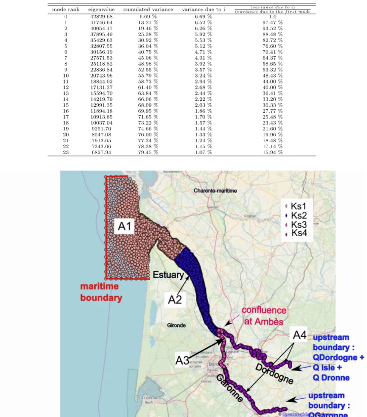
southwest France. Created from the confluence of two rivers (Garonne and Dordogne rivers), it extends 75 km to reach the mouth of the estuary at the Atlantic coast-line (Fig. 1). On average, it is oriented from south-east to north-west in a valley, and its width ranges from 1 km near Bordeaux to 15 km at the coast. The Gironde estuary can be divided [28] into three subdomains: the upstream river area, the central estuary area and the downstream offshore area [29]. The estuary can be clas-sified as macrotidal, hypersynchronous, and with an asymmetric tide (4 h for the flood and 8 h 25 min for the ebb). The tide in the Bay of Biscay is semidiur-nal, with a period of 12 h 25 min and is dominated by the principal semidiurnal lunar (M2) component. The open ocean induces a strong tidal forcing with a tidal amplitude near the mouth of the estuary ranging from 2.2 to 5.4 m over the spring-neap cycle. The Garonne (resp. Dordogne) river discharge typically ranges from 50 (resp. 20) up to 2 000 (resp. 1 000) m3.s-1. During
flood events, the Garonne flow rate occasionally exceeds 5 000 m3.s-1. The economic importance of the Gironde
estuary is evidenced by the presence of large cities and
ports, including the city of Bordeaux and the Harbor of Bordeaux, as well as by the presence of various indus-tries, such as the Blayais nuclear power plant, fisheries and tourism activities. The flooding risk has been a ma-jor concern for authorities along the Gironde estuary [1] for a long time, as shown by historical documents dating from the XIIIth century. The most damaging
flood occurred in April 1770, when about 24 000 km2
were covered by water along the Garonne river and the Gironde estuary, causing about 4,669 million euros in damage exclusively in the city of Bordeaux (35 million euros using purchasing power parity for primary goods). From this point, flood protection structures were built to limit the consequences of flooding. However, this did not prevent strong floods in 1835, 1855 and 1856. In 1930, floods caused the destruction of 1 000 houses and more than 300 casualties. In recent decades, three no-table events were observed: the December 1981 event, which was caused by strong river discharges during high tides, and the Lothar and Martin storms in 1999 and Xynthia in 2010 [30].
2.1.2 Shallow water equations in Telemac2D
TheSWEare commonly used in environmental hydro-dynamics modelling. They are derived from the Navier-Stokes equations and express mass and momentum con-servation averaged in the vertical dimension. The non-conservative form of the equations are written in terms of the water depth (h [m]) and the horizontal compo-nents of velocity (u and v [m.s-1]).
∂h ∂t + ∂ ∂x(hu) + ∂ ∂y(hv) = 0 (1) ∂u ∂t + u ∂u ∂x + v ∂u ∂y =−g ∂H ∂x + Fx+ 1 hdiv ( hνe−−→grad (u) ) (2) ∂v ∂t + u ∂v ∂x+ v ∂v ∂y =−g ∂H ∂y + Fy+ 1 hdiv ( hνe−−→grad (v) ) (3) where: Fx=− g Ks2 u√u2+ v2 h43 − 1 ρw ∂Patm ∂x +1 h ρair ρw Cd Uw,x √ U2 w,x+ Uw,y2 (4)
Fy=− g Ks2 v√u2+ v2 h43 − 1 ρw ∂Patm ∂y +1 h ρair ρw Cd Uw,y √ U2 w,x+ Uw,y2 (5)
and ρair/ρw [kg.m-3] are the air/water density, Patm
[Pa] is the atmospheric pressure, Uw,x and Uw,y [m.s-1]
are the horizontal wind velocity components, Cd [-] is
the wind drag coefficient that relates the free surface wind to the shear stress, Ks[m
1
3.s-1] is the river bed and
floodplain friction coefficient, using the Strickler formu-lation [31]. Fxand Fy [m.s-2] are the horizontal
compo-nents of external forces (friction, wind and atmospheric forces), H [m NGF69] is the water level (h = H− zf
if zf [m NGF69] is the bottom level) and νe [m2.s-1] is
the water diffusion coefficient. div and−−→grad are
respec-tively the divergence and gradient operators. To solve the system of equations Eq. (1) to Eq. (3), initial condi-tions h(x, y, t = 0) = h0(x, y); u(x, y, t = 0) = u0(x, y); v(x, y, t = 0) = v0(x, y) are provided. Boundary condi-tions (BC) both at the coastline (slip and impermeabil-ity conditions) and at the upstream and downstream boundaries (h(xBC, yBC, t) = hBC(t)) are also given.
In the present study, the SWE are solved with the par-allel numerical solver Telemac2D (www.opentelemac.org) with an explicit first-order time integration scheme, a fi-nite element scheme and an iterative conjugate gradient method [3]. In the following, we will take into account parametric uncertainties, that are due to the stochastic nature of the atmosphere-surface system. These include the forcing fields and epistemic uncertainties that come from a lack of knowledge concerning the physical pro-cesses of the hydrodynamic system, leading to a simpli-fied parametrization, such as friction or turbulence, but also the imperfect description of the system, such as the geometry of the river. These uncertainties can be repre-sented by independent scalars (friction coefficients) or timeand/orspace correlated discretized fields (fluvial, atmospheric and maritime forcings).
2.1.3 The Gironde estuary numerical model
A hydrodynamic numerical model of the Gironde estu-ary (Fig. 1), based on Telemac2D and on a bathymetry / topography field (Fig. 2), is used operationally to com-pute the water depth and velocity in the estuary and along the Garonne and Dordogne rivers. The maritime boundary is located in the Gascogne Gulf, 35 km away from le Verdon. The upstream boundaries are located at La Réole on the Garonne River and at Pessac on the Dordogne River. It should be noted that inflows from the Isle and Dronne rivers are artificially injected at
Pessac [4] and that floodplains are not taken into ac-count. The operational numerical model used by FFS GAD covers about 125 km from east to west, features 12838 finite elements and is composed of 7351 nodes (coarse mesh). Refined meshes (27546 nodes, 106450 nodes and 418314 nodes) were built for a convergence study. It was shown that mesh convergence is obtained for water levels (using a 5 cm error threshold) in the en-tire estuary except in the fluvial areas for meshes with more than 106450 nodes. The 418314 node fine mesh was thus used in the following for SA. Hydrological up-stream forcings for the Dordogne and Garonne rivers are provided by the DREAL (Direction Régionale de l’Environnement, de l’Aménagement des Territoires et du Logement) Nouvelle Aquitaine at a 1-hour time step. Surface wind velocity and pressure fields from the re-gional meteorological model ALADIN [32] are provided by Meteo-France at a 3-hour time step. Water levels at the maritime boundary are the sum of the predicted astronomical tide and surge levels; these data are also provided in real-time by Meteo-France every 10 to 15 min. The friction coefficient is uniformly defined over 4 areas as shown in Fig. 1. The model calibration was achieved during the non-flooding 2003 event to optimize either the water level Root Mean Square Error (RMSE, Eq. (6)) or the Nash criteria at high tide (NashHT,
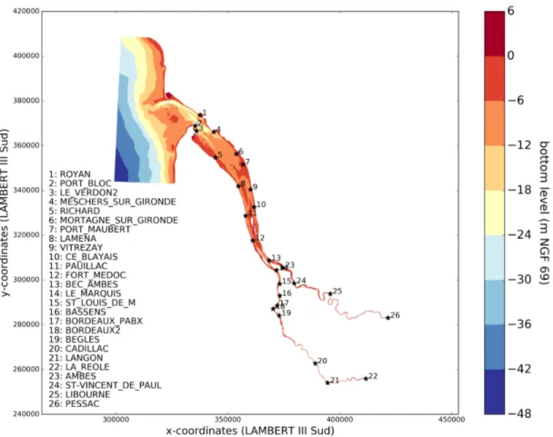
Eq. (7)) computed between simulated and observed wa-ter levels available at the 12 stations among the 26 sta-tions of interest shown with red stars in Fig. 2. Two sets of friction coefficients were obtained from the calibra-tion and are presented in Table 1. The resulting RMSE and NashHT scores for the 2003 event are presented in
Table 2 along with the evaluation scores for the 1999 flooding event. The NashHT (Eq. (7)) is evaluated at
high tide and the RMSE (Eq. (6)) (resp. RMSEHT) is
evaluated by summing over the entire flood event (resp. at high tide): RM SE = v u u t 1 n n ∑ i=1 (Hi− cHi)2 (6) N ashHT = 1− ∑n i=1(Hi− cHi)2 ∑n i=1(cHi− H)2 , (7)
where n is the time index, Hiand cHi are the simulated
and observed water levels and H the time-averaged ob-served water levels. As expected, the RMSE and NashHT
scores are significantly better for the 2003 non-flooding calibration event than for the 1999 flooding evalua-tion event. The water level RMSE reaches 16 cm at Le Verdon and 36 cm at Laména in 2003 and 2.0 m
at Le Verdon and 1.49 m at Laména for the overflow-ing event in 1999. These errors remain higher than the target 10 cm precision expected by FFS GAD. These re-sults are computed over past events in reanalysis mode using perfect meteorological and hydrological forcing. Additional errors due to imperfect forecasting are ex-pected in operational mode, especially with increasing lead time [4]. The scores obtained for calibration and evaluation events, especially in flooding conditions, ad-vocate further improvement of the Gironde model with the assimilation of observed water levels.
The wind drag coefficient formulates the wind shear stress at the free surface from the wind velocity [33]. A uniform and constant value was chosen here (Cd =
2.14 10−3) consistently with the calibration of the surge level numerical model for the Atlantic Ocean, English Channel and North Sea [34].
2.2 Computation of sensitivity indices
2.2.1 Variance decomposition and Sobol’ indices
Sobol’ indices [35] measure the contributions of the dif-ferent independent inputs X1, X2, . . . , Xd and their
in-teractions in the variance V(Y) of the output Y = f (X) with X = (X1, X2, . . . , Xd), E((f (X))2) < ∞ and f
the model.Si = V (Y )Vi is the first-order Sobol’ index of
Xi, representing the normalized elementary
contribu-tion of Xi to V (Y ). Si,j = V (Y )Vi,j is the second-order
Sobol’ index of Xiand Xj, representing the normalized
contribution of the interaction between Xi and Xj to
V (Y ), and so on. As described in Appendix A, using Eq. (8): 1 = ∑ i⊆Id Si+ ∑ {i,j}⊆I2d j>i Si,j+ . . . + S1,2,...,d = ∑ u⊆Id Su (8)
where: Id={1, . . . , d} is the set of input indices, the
to-tal Sobol’ index STi gathering all contributions related to Xi is then defined as:
ST i= Si+ ∑ j∈Id j>i Si,j+ . . . + S1,2,...,d= ∑ u⊆Id u∋i Su (9)
It should be noted that ∑iSi = 1 if there is no
interaction between the input parameters.
2.2.2 Implementation of Sobol’ indices computation
The main steps for the stochastic estimation of the Sobol’ indices of the different independent inputs X1, X2, . . . , Xdwith X = (X1, X2, . . . , Xd) are described in
Ap-pendix B according to [10], which the reader can refer
to for more details.
It should be noted that the calculation of the first and total Sobol’ indices for an ensemble of size N requires the integration of two independent samples. Given d un-certain variables and Ne perturbed members for each
variable, the total number of simulations is thus N =
Ne(d + 2).
If (Xi)i=k,,k+m correspond to the m uncertain modes
of a field input, the contribution of each mode can be estimated separately with the methodology described in Appendix B, but also the whole contribution of the field input. If kmdenotes the number of uncertain field
variables whose contribution is estimated in addition to the contribution of each mode, then the total number of simulations is N = Ne(d + 2 + km).
2.3 Ensemble generation with field inputs
2.3.1 Uncertain space for SA in the Gironde estuary
The GSA study was carried for the 7-day February 2003 event with a tide coefficient in the range [43 ; 90], Dor-dogne upstream discharge (resp. Garonne) in the range [600 ; 2200] m3.s-1(resp. [1200 ; 5900] m3.s-1).
The present study has d = 8 uncertain sources: the 4 zone-distributed scalar friction coefficients (Ks1, Ks2, Ks3, Ks4), the scalar wind drag coefficient Cd, and the time-dependent boundary conditions at the hydrolog-ical limits (QDOR and QGAR for the Dordogne and Garonne rivers respectively) and at the maritime limit (CLMAR). Additional sources of uncertainty, such as space- and time-varying meteorological forcing or bathymetry, exist and have not been considered in the study. The uncertain input vector is denoted by X = (Xi)i∈I8
where X1 = Ks1, X2 = Ks2, X3 = Ks3, X4 = Ks4, X5 = Cd, X6 = QDOR, X7 = QGAR and X8 =
CLMAR. The QoI is the water level defined over the simulation domain at a given time, with 26 stations that are of particular interest (see Fig. 2). The water level at a given location is a scalar denoted by Y in the following.
The wind drag coefficient and friction coefficients are supposed to follow uniform distributions with ranges described in Table 1. [33] presents a review of paramet-ric formulations of the wind drag coefficient based on [36], [37], [38]. These parametric formulations were used for the Gironde case using climatological wind intensi-ties (Climate Forecast System Reanalysis from NOAA) to define the range for the Cd uniform distribution. The ranges of the friction coefficients are chosen so as to include the calibration values for the 2003 event us-ing both the NashHT and RMSE criteria. The interval
corresponds to the commonly accepted uncertainty on friction for engineering studies.
The time-dependent hydrological forcing is assumed to be perturbed by an additive centered Gaussian pro-cess q(t). The covariance of q(t) is defined by a squared exponential kernel κ(t, t′) = σ2exp(−ℓ−2(t−t′)2), where ℓ is the correlation time scale estimated from
obser-vations over the 1981-2016 period, and the standard deviation σ is the amplitude of the perturbation. The time dependent maritime forcing is also assumed to be perturbed by an additive Gaussian Process h(t) with a gaussian covariance function. A truncated form qp(t)
(resp. hp(t)) of q(t) (resp. h(t)) is formulated with aKL
decomposition [20] of q(t) (resp. h(t)).
Numerically, as explained in Appendix C, the eigen-function problem defined by the Fredholm equation is approximated by the eigenvector problem defined over the discretized time series{t1, t2, . . . , tN}:
KΦi= λiΦi (10)
where Φi = (ϕi(t1) . . . ϕi(tN))T, K = (κ(ti, tj))1≤i,j≤p
and (λi, ϕi) are the ith eigenvalue and eigenfunction of
κ, the solution of the Fredholm equation [39].
The solution (λi, Φi) of Eq. (10) is obtained from a
sin-gular value decomposition (SVD) and contributes to the truncated expansion of q(t) (and h(t)) discretized over the discretized time series:
qp= (qp(t1), . . . , qp(tN))T = p ∑ i=1 √ λiΦiϵi. (11)
where ϵi are independent standard Gaussian variables.
Last but not least, based on the property∑pi=1λi = σ2,
the degree of truncation p is chosen such that the frac-tion of the total variance∑pi=1λiσ−2 exceeds a
thresh-old the closest to one.
Sampling the perturbation q(t) (resp. h(t)) associ-ated with the time-dependent hydrological (resp. mar-itime) forcing over the discretized time series{t1, t2, . . . , tN}
sums up sampling the random vector qp (resp. hp), as
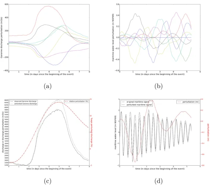
sampling p independent standard Gaussian variables. Fig. 3-a and Fig. 3-b present a set of 7 perturbations of the boundary condition q(t) at the Garonne upstream location and h(t) at the maritime boundary.
The boundary condition resulting from the afore-mentioned perturbed signal is displayed in Fig. 3-c for the Garonne and in Fig. 3-d for the maritime bound-ary. The autocorrelation time scale was estimated for about 10 discharge signals during major flood events on the Garonne and Dordogne rivers. The correlation time scales ℓQGARand ℓQDORare thus set to 3 days for
the 2003 event and the correlation time scale ℓCLMAR
is set to 6 hours (approximately half a tidal cycle) for
the maritime boundary. The amplitudes σQDOR and σQGARof the perturbations of the upstream discharges
are set proportional (20 %) to the observed discharges as the uncertainties of the rating curves used to trans-late the water levels into discharges are larger for high flow time series. The amplitude σCLMAR of the
mar-itime boundary condition perturbation is set to 50 cm, representing the sum of the uncertainties in surge lev-els and in the predicted offshore tide, at the maritime boundary of the numerical model. The KL decompo-sitions of the hydrological and maritime forcings are respectively truncated to pQDOR = pQGAR = 4 and pCLMAR = 7 modes, retaining respectively 90 % and 45 % of the Gaussian process variability. This value, associated to ℓCLMAR, will be discussed in Sect. 3.4.
Moreover, the KL modes will be either aggregated or treated separately in the following for Sobol’ indices formulation. The GSA is thus carried out in an un-certain space described by 20 variables: Ks1, Ks2, Ks3, Ks4, Cd, 4 modes for each hydrological boundary condi-tion (QGAR and QDOR) and 7 modes for the maritime boundary condition CLMAR.
2.3.2 High Performance Computing resources
The GSA for the 2003 event was performed using both coarse and fine meshes. Due to computational constraints, it was only carried out over one tidal cycle with the fine mesh. Yet the conclusions drawn for the GSA over this period with the fine mesh are similar to those drawn for the coarse mesh over the 7-day event. As a consequence, in the following, illustrations for the GSA are given for the coarse mesh model. Computational resources for the GSA are given in Table 3. For the fine mesh, the convergence of the GSA results was investigated with increasing number of members Ne ranging from 100
to 10000. The Sobol’ indices reach convergence for all variables over the simulation time period (not shown) from Ne = 2000. The simulations were performed on
the HPC resources from GENCI-IDRIS (grant 2017-A0030110292).
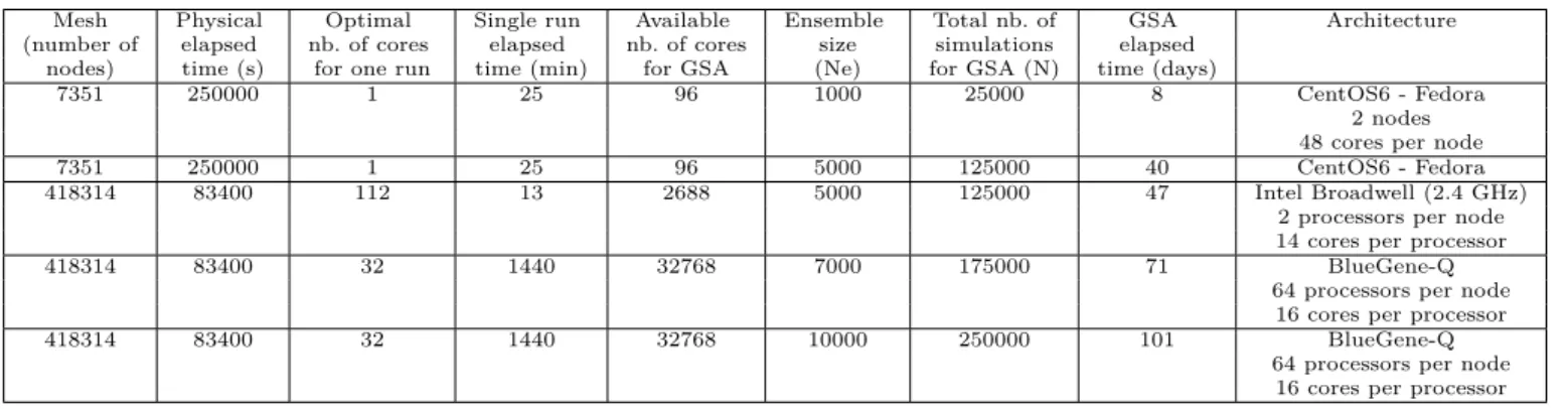
For coarse and fine meshes (Table 3 - Col. 1), the sim-ulated period is indicated in Table 3 - Col. 2. For each HPC architecture (Table 3 - Col. 9), a scalability study was performed for a single run with domain decomposition: the optimal number of cores is shown in Table 3 -Col. 3 along with the elapsed time in Table 3 --Col. 4. The GSA involves both domain decomposition and task parallelism. The total number of available cores for the GSA is shown in Table 3 - Col. 5. As Sobol’ indices are computed for field inputs considering the contribution of each mode only and also the whole contribution of the uncertain variable, the ensemble size Ne and the
total number of simulations N are given in Table 3 -Col. 6 and -Col. 7 respectively. Finally, the elapsed time for the GSA is given in Table 3 - Col. 8.
3 GSA results
The GSA study was carried for the 7-day February 2003 event with a tide coefficient in the range [43 ; 90], Dor-dogne (resp. Garonne) upstream discharge in the range of [600 ; 2200] m3.s-1 (resp. [1200 ; 5900] m3.s-1).
3.1 Performance of the ensemble
3.1.1 Description of the criteria
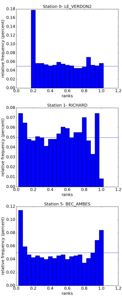
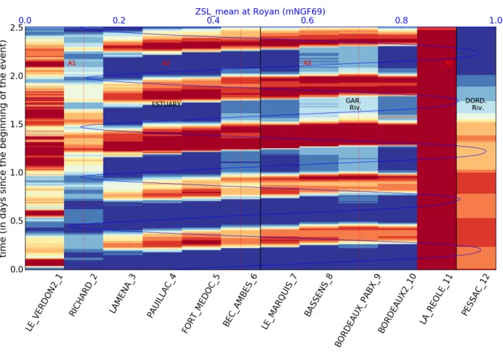
The performance of the ensemble forecasts is commonly assessed with criteria such as consistency and reliabil-ity [40]. The former measures the average spread of an ensemble compared to observations, whereas the latter generally reflects the accuracy of a forecast model. The consistency criterion characterizes the coherence between the distribution of the ensemble members and a set of observations through the use of the rank his-togram [41] for a given simulation time or over a simula-tion period. The ensemble values are ranked in classes, and the occurrence of the observed value within these classes is computed and represented with a rank his-togram. Fig. 4 displays the rank histogram at stations Le Verdon, Richard and Bec d’Ambès for all time steps during the 2003 event. It is expected to be flat when the ensemble members and the observations follow similar distributions, U-shaped when the ensemble is under-dispersive, and bump-shaped when the ensemble is over-dispersive. Here, the occurrence is normalized by the ensemble size and is displayed in Fig. 5 with a blue-red color bar along the curvilinear abscissa (x-axis) of 12 observing stations as a function of time (y-axis). This time and space distributed representation allows the de-termination of when and where the ensemble is consis-tent with the observations (ranks uniformly distributed from 0.1 to 0.9) or not (extreme rank values equal to 0 when the ensemble over estimates water levels, and rank values equal to 1 when the ensemble under esti-mates water levels).
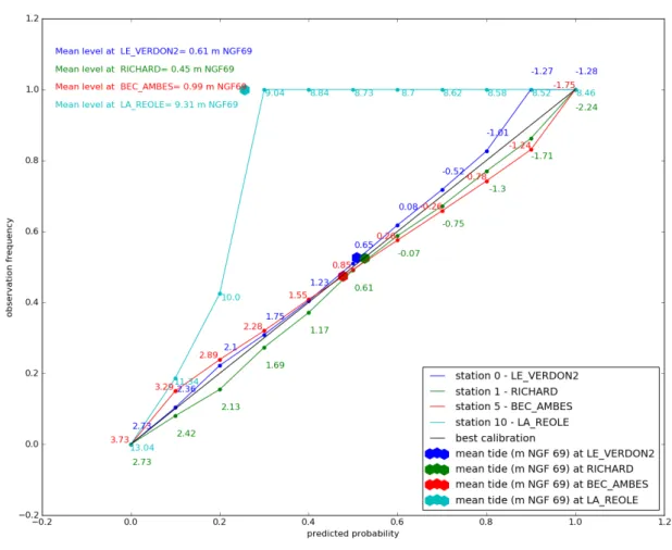
The reliability criterion evaluates the coherence between the forecasted and the observed probabilities of an event [42]. An event is defined as Z >= ZT, where Z is the
random value simulated in the ensemble and ZT is the
threshold value. The reliability plot represents the ob-servation probability for the events with respect to the simulated probability. The ensemble is reliable if the re-lation follows the first bisector line; it is under or over
dispersive otherwise. The reliability criterion for 4 ob-serving stations (Le Verdon, Richard, Bec d’Ambès and La Réole) is represented in Fig. 6. Over each curve, the observation quantiles (q10 to q90) are represented
with circles (q50 represented by a larger symbol).
Reli-ability curves under (resp. above) the perfect reliReli-ability diagonal curve reveal an over-predictive (resp. under-predictive) ensemble.
3.1.2 Interpretation of water level ensemble performance
Considering both performance criteria in Fig. 4, Fig. 5 and Fig. 6, it appears that the performance of the en-semble is closely related to the tidal cycle and the lo-cation in the estuary. At Le Verdon (resp. Richard), at the mouth of the estuary, the reliability curve (blue (resp. green) curve) shows that the ensemble is slightly under- (resp. over-) predictive for all quantiles with wa-ter levels that are under- (resp. over-) estimated. Con-sidering the corresponding locations of Fig. 5 for each of them shows respectively a predominance of red and blue nuances independent of the tidal cycle. For wa-ter levels lower than the mean tide wawa-ter level, this can be explained at Le Verdon by a truncated observed signal during the 2003 event. Moreover, calibration re-sults (Table 2) have shown the trend of the numerical model to under-estimate water levels at Le Verdon and to over-estimate them at Richard during flood tide, as the mean error for high tides are respectively negative (-12 cm at Le Verdon) and positive (+21 cm at Richard). In the middle part of the estuary, from Laména to Bor-deaux, Fig. 4 shows a tide-dependent rank. The ensem-ble is over-predictive at low tide and under-predictive at high tide, as suggested in Fig. 6 by the reliability curve at Bec d’Ambès (red line). The Bec d’Ambès re-liability curve is under the perfect diagonal rere-liability curve for water quantiles lower than the mean tide level and above this curve for quantiles higher than the mean tide level. This reflects calibration choices for a better representation of high tides leading to under-dispersive behavior. Indeed, the reliability curve exhibits smaller distances to the diagonal for higher water levels than for lower ones. At the upstream part of Garonne and Dordogne rivers, Fig. 4, Fig. 5 and Fig. 6 show a strong under-predictive signature of the ensemble at La Réole and an over-predictive signature at Pessac (for the end of the storm). This highlights the need for a more re-fined mesh in the fluvial part of the model.
The ensemble performance has been assessed. It shows that the over/under predictive signature or non-reliability is directly linked to the numerical model calibration or to the mesh refinement in the fluvial areas.
3.2 Water level probability density function
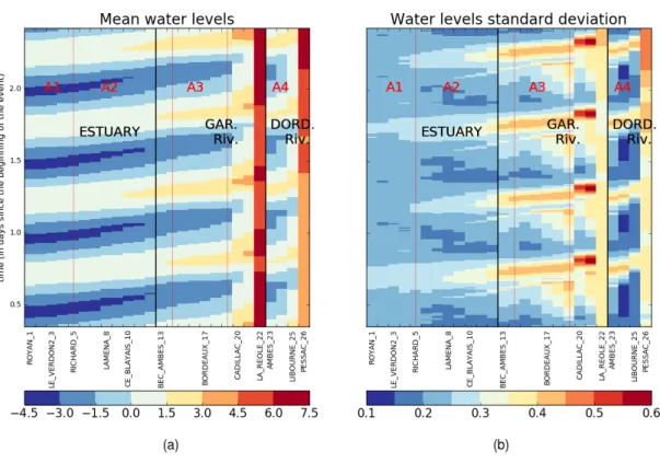
The water level mean and standard deviation are dis-played with a blue-red color bar along the curvilinear abscissa (x-axis) of the 26 stations of interest as a func-tion of time (y-axis) in Fig. 7. Fig. 7-a shows the en-semble mean water level; it illustrates the propagation of tides from the mouth of the estuary to the upstream part of the Garonne and Dordogne rivers. The hyper-synchronic characteristic of the Gironde estuary due to a funnel effect leads to the amplification of high tides in the estuary from the decreasing water depth in bathymetry. The absolute differences of the median with 95%-quantile and 5%-quantile (not shown) shows a nearly perfect symmetry of the distribution of QoIs between its extreme quantiles. The standard deviation plotted in Fig. 7-b increases from 20 cm at Royan to 45 cm at Pessac and La Réole for high tides.
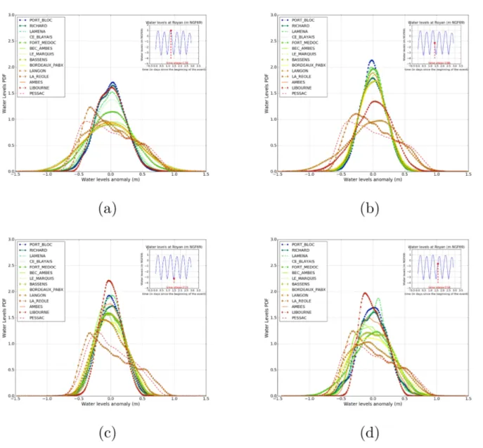
Fig. 8 displays the PDF of water level anomalies (with respect to the ensemble mean) at the storm peak (a), ebb tide (b), low tide (c) and flood tide (d) for 14 ob-serving stations (blue curves for the maritime bound-ary, green for the estubound-ary, yellow, orange and red for the Garonne and Dordogne rivers). Upstream of the fluvial areas, the PDF is asymmetric for all times with a me-dian value of about -40 cm, a mean value of 10 cm, and a fat tail for positive anomalies at La Réole, Langon and Pessac. Upstream of La Réole, Langon and Pessac, the PDF is symmetric on the Garonne and Dordogne rivers with a standard deviation of about 1.8 m for the flood rise and storm peak, leading to anomalies up to 1 m and a standard deviation of about 0.6 m for ebb tide and low flow. Along the estuary and in the maritime area, the PDF is rather symmetric. The standard de-viation decreases from the confluence at Bec d’Ambès to the mouth of the estuary. The standard deviation over the estuary, except in the fluvial area, is larger for flood tide and storm peak than for ebb tide and low flow. This behavior can be explained by the hypersyn-chronous shape of the estuary which amplifies pertur-bations from the maritime boundary conditions along the estuary at flood tide. Moreover, it reflects respec-tively the predominance of the gaussian perturbation of the maritime signal and the uniform perturbation of the Strickler coefficient with a non-linear behavior in the fluvial part.
3.3 Global sensitivity analysis indices for aggregated modes
3.3.1 Temporal analysis
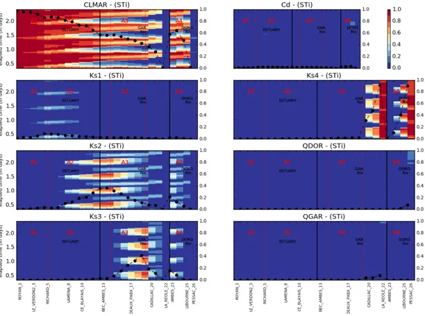
Sobol’ indices are displayed with a blue-red color bar for the 8 uncertain inputs Xi (Sect. 2.3.1) in Fig. 9, along
the curvilinear abscissa (x-axis) and over time (y-axis). The total Sobol’ indices are plotted for each input vari-able. Blue/red means small/large Sobol’ indices for Xi.
For the 2003 event studied here, Fig. 9 clearly shows the predominance of the maritime boundary conditions and the dependency of all variables on the tidal signal. The wind drag coefficient, the hydrological boundary conditions and the friction coefficient in area A4 have
no influence on the water level variability except at the upstream location of the Garonne and Dordogne rivers. Over the maritime area A1, the water level variance
is explained by the variance in the maritime bound-ary condition with Sobol’ indices close to 1 from Royan (station 1) to Richard (station 5) near the mouth of the estuary. It should be noted that the fraction of the water level variance that is not explained by CLMAR is explained by Ks1. In estuarian area A2, CLMAR and
Ks2 are the most significant sources of uncertainty, with a large predominance of CLMAR at high tide. At low tide, the Sobol’ index for Ks2 reaches 0.8. The influ-ence of the maritime boundary condition decreases from Fort-Médoc (in A2) to the confluence at Bec d’Ambès
(in A3) and the influence of Ks2 and Ks3 increases. For
this event, in area A4, the influences of CLMAR and
Ks4 are alternatively predominant in coherence with the tidal signal. At La Réole and Pessac, Sobol’ index for Ks4 reaches 0.8. It should be noted that the dif-ference between total and first order indices, represent-ing interactions of Xi with other uncertain variables,
has been computed for all uncertain variables. As it is nearly equal to 0, it can be concluded that, for the 2003 storm, no interactions are detected between any input variable Xi. Total Sobol’ indices and ranks are
time-averaged and plotted in Fig. 10 along the curvilinear abscissa (x-axis) and for all Xi(y-axis). As expected, for
the 2003 event, the maritime boundary conditions have a predominant impact along the entire domain, with the significant influence of friction coefficients, while hydro-logical boundary conditions have a limited impact to the upstream locations of the Garonne and Dordogne rivers.
3.3.2 Global sensitivity analysis space mapping
Figs 11-a (resp. -c) and 11-b (resp. -d) display maps of total Sobol’ indices over the entire mesh of the variable
X8 = CLMAR (resp. X1 = Ks1), at the storm peak
and at low tide respectively, for the 2003 event. These maps show the homogeneity of the total Sobol’ indices geographical repartition and confirm that the conclu-sions drawn previously for the 26 locations of interest can be generalized for all points located in A1, A2, A3
and A4. The same maps have been obtained for all
un-certain variables for the storm peak, ebb tide, low tide and flood tide, but are not shown here. As formerly observed, for the 2003 event, the wind drag coefficient (Cd), Dordogne river discharge (QDOR) and Garonne river discharge (QGAR) have a very small influence over the tidal cycle along the estuary. As 2003 event is a flood event for both rivers, further investigation is needed to confirm this conclusion. The uncertainty in the maritime boundary condition is predominant, espe-cially during the flood tide and storm peak (at Royan) (Fig 11-a) along the estuary except at the upstream part of the Garonne and Dordogne rivers (in A4), where
friction coefficient Ks3 is the most dominant uncertain variable. Ks1 (displayed in panels c- and d-), Ks2 and Ks4 show no influence during the storm peak. During ebb tide, the influence of CLMAR propagates along the Garonne and Dordogne rivers, while the upstream parts of the rivers remain fully under the influence of Ks3. At low tide, Fig. 11-b shows that the influence of CLMAR returns to the middle part of the estuary in A2, whereas
Ks1 (resp. Ks2) is the most dominant uncertain vari-able farther downstream (resp. upstream), consistent with the tidal signal. The influence of Ks3 in the up-stream part of the Dordogne and Garonne rivers prop-agates to A4. The Gironde Estuary hydrodynamics are
the result of interplays between time and/or space de-pendent processes, such as friction, convergence of the estuary and maritime and fluvial usptream boundary conditions, but also of the memory of the state of the system. UQ and GSA help to identify and understand the evolution of complex physical processes that drive the Gironde estuary and are not entirely intuitive, in particular, when considering their phase with the tidal cycle.
3.4 Focus on the eigenmodes of the maritime boundary forcings
A GSA study dedicated to the maritime boundary forc-ing was performed considerforc-ing each eigenmode of the KL decomposition for the 7-day 2003 event. The other parameters (Ks1, Ks2, Ks3, Ks4, QGAR and QDOR) are not perturbed and their associated values are their mean values. Table 4 shows the variance associated with each orthogonal function of the KL decomposition of
the Gaussian correlation function with its time scale set to 6 hours (half-tide). No clear predominance of the first modes is observed with about 6 % of the input variance explained by the first 4 modes and 1 % for the follow-ing 19 modes. The accumulated variance explained by the first 7 modes kept for the GSA is about 45 %. The Sobol’ indices associated with these modes are plotted in Fig. 12. Their contributions are linked to the tide cycle but are asynchronous. The influence of the eigen-modes decreases from the mouth of the estuary to the upstream part of the rivers with respect to the peri-odic tide signal. Modes 2, 3, 4 and 5 have major contri-butions, their respective Sobol’ indices reaching 30 %, whereas modes 6 and 7 have less influence during the second part of the storm event and mode 1 has no influ-ence on water levels except at the end of the event when its total Sobol’ index reaches 20 %. The uncertainty in the tide and surge level was estimated by [43] to be re-spectively 5 cm and 40 cm for a 36-hour lead time. This suggests dividing the maritime signal uncertainty into a deterministic tidal contribution and a stochastic surge level contribution caused by the meteorological forc-ings [44] as well as the tide/surge level interactions [45] through surge levels. Further work should thus focus on separating the tidal signal from the surge level signal. The correlation time scale calculated from the surge level time series provided by Meteo-France is about 2.1 days. Only 14 eigenmodes (resp. 4) are required to rep-resent 99 % (resp. 90 %) of the total variance of the signal, as shown in Fig. 13.
4 Conclusions and perspectives
The Telemac2D numerical model used for operational flood forecasting by FFS GAD in the Gironde estuary was used for a GSA based on ANOVA to estimate the Sobol’ indices over a 7-day storm event in 2003. It was shown that the maritime boundary conditions drive the dynamics of the estuary.
Moving from the mouth of the estuary to the upstream part of the Garonne and Dordogne rivers, the influence of the friction coefficient increases, and the hydrologi-cal forcing has a very lohydrologi-cal influence upstream in the rivers. This GSA study allows the identification of the most significant sources of uncertainty. Once identified, these uncertainties should be reduced, for instance with a data assimilation algorithm such as Ensemble Kalman Filter, in order to improve the water level in the estu-ary in simulation and forecast mode. A perspective for this study is to take into account uncertainties in the surface forcing atmospheric fields (wind and pressure). Further work should also focus on the formulation of a surrogate model for the 2D Gironde hydraulics model
for high flow discharges in order to reduce the cost of the GSA and the ensemble assimilation. Gaussian Pro-cess or Polynomial Chaos surrogates have been used for UQ and GSA in the context of hydraulics ([46], [23]). Both methods proved efficient for metamodelling of the SWE with the 1D solver Mascaret ([47], [48]) for GSA with Sobol’ indices and covariance matrix esti-mation. A polynomial surrogate was also implemented for Telemac2D on the Garonne river and allowed for a cost-reduced computation of the sensitivity indices [23]. This work should be extended to the Gironde estu-ary taking into account scalar and field uncertainties. The proposed surrogate modeling and data assimila-tion approaches would meet this need and would result in a reduced-cost ensemble based data assimilation al-gorithm to reduce major sources of uncertainties and improve water level forecasting in the Gironde estuary.
A Appendix A
Sobol’ indices [35] measure the contributions of the different in-dependent inputs X1, X2, . . . , Xdand their interactions in the variance V(Y) of the output Y = f (X) with X = (X1, X2, . . . , Xd),
E((f (X))2) <∞ and f the model. They are based on the
Ho-effding decomposition of f [49], f (X) =f∅+ ∑ i⊆Id fi(Xi) + ∑ {i,j}⊆I2d j>i fi,j(Xi, Xj) + . . . + f1,2,...,d(X1, X2, . . . , Xd) = ∑ u⊆Id fu(Xu) (12)
where Id={1, . . . , d} is the set of input indices, f∅= E(Y ) is the expectation of Y (here the average of all values Y can take), fi(Xi) = E(Y|Xi)−f∅is the elementary contribution of Xito
f (X), and fi,j(Xi, Xj) = E(Y|Xi, Xj)−fi(Xi)−fj(Xj)−f∅ is the contribution of the interaction between Xi and Xj to
f (X).
From Eq. (12) and using the orthogonality condition E(fifj) = 0 if i̸= j, the variance of Y is:
V (Y ) = ∑ i⊆Id Vi+ ∑ {i,j}⊆I2d j>i Vi,j+ . . . + V1,2,...,d= ∑ u⊆Id Vu (13)
where Vi = V (fi(Xi)) is the elementary contribution of Xi to V (Y ), Vi,j = V (fi,j(Xi, Xj)) is the contribution of the interaction between Xi and Xj to V (Y ), and so on. Dividing Eq. (13) by V (Y ) leads to Eq. (8).
B Appendix B
This appendix describes the main steps for the stochastic esti-mation of the Sobol’ indices of the different independent inputs X1, X2, . . . , Xdwith X = (X1, X2, . . . , Xd) according to [10].
1. Step 1: generation of two ensembles of size Ne for the nor-malized input parameters set (x1, x2, . . . , xd). The first (resp. second) (Ne, d) matrix is denoted by A (resp. B) (Eq. (14) (resp. (Eq. (15)))). The space filling strategy is carried out with a Sobol’ sequence rather than a classical Monte-Carlo strategy:
A = x(1)1 x(1)2 · · · x(1)i · · · x(1)d x(2)1 x(2)2 · · · x(2)i · · · x(2)d · · · · · · · · · · · · · · · · · · x(N e1 −1)x(N e2 −1)· · · x(N ei −1)· · · x(N ed −1) x(N e)1 x(N e)2 · · · x(N e)i · · · x(N e)d (14) B =
x(N e+1)1 x(N e+1)2 · · · x(N e+1)i · · · x(N e+1)d x(N e+2)1 x(N e+2)2 · · · x(N e+2)i · · · x(N e+2)d
· · · · · · · · · · · · · · · · · · x(2N e1 −1)x(2N e2 −1)· · · x(2N ei −1)· · · x(2N ed −1) x(2N e)1 x(2N e)2 · · · x(2N e)i · · · x(2N e)d (15) 2. Step 2: definition of d matrices Ciformed by all columns of A except the ith column taken from B [49].
3. Step 3: computation of the model output (and QoI) yA(resp.
yB and yCi with i = 1, , d), for all the input values in the sam-ple matrix A (resp. B and the d matrices Ci), obtaining (d + 2) vector outputs of dimension Ne: yA = f (A), yB = f (B),
yCi = f (Ci) with i = 1, , d.
[49], [50] and [51] describe the best approach to compute si-multaneously Siand STi for each input variable.
In this study, the following estimators have been chosen for: VXi(EX˜i(Y|Xi)) = 1 N ∑N j=1y (j) B ( yC(j) i − y (j) A ) , EXi(VXi(Y|Xi)) = 1 2N ∑N j=1 ( y(j)A − y(j)C i )2 and V (Y ) =N1∑Nj=1 ( yAj )2 − f2 0 with f2 0 = 1 N ∑N j=1y j Ay j B.
Anomalies due to an uncertain variable Xi corresponding to the normalized uncertain variable xiare defined as yCi− yA and represent the part of the QoIs output resulting from Xi only.
If (Xi)i=k,,k+m correspond to the m uncertain modes of a field input, the contribution of each mode can be estimated separately with the methodology described above. The whole contribution of the field input can also be estimated by process-ing the uncertain variable modes in one block and by definprocess-ing a matrix Ck formed by all columns of A except the kth to (k + m)thcolumns taken from B.
C Appendix C
A truncated form qp(t) (resp. hp(t)) of q(t) (resp. h(t)) is for-mulated with aKLdecomposition [20] of q(t) (resp. h(t)): qp(t) = p ∑ i=1 √ λiϕi(t) ϵi (16)
where ϵiare independent standard Gaussian variables and (λi, ϕi) are the itheigenvalue and eigenfunction of κ, the solution of the
Fredholm equation [39]: ∫
κ (t, τ ) ϕi(τ ) dτ = λiϕi(t) (17)
with∫ϕi(t)ϕj(t)dt = δi,j.
References
1. Jaak Monbaliu, Zhongyuan Chen, Didier Felts, Jianzhong Ge, Francois Hissel, Jens Kappenberg, Siddharth Narayan, Robert J Nicholls, Nino Ohle, Dagmar Schuster, et al. Risk assessment of estuaries under climate change: lessons from western europe. Coastal Engineering, 87:32–49, 2014. 2. Maryam Golnaraghi. Institutional partnerships in
multi-hazard early warning systems: a compilation of seven national good practices and guiding principles. Springer Science & Business Media, 2012.
3. Jean-Michel Hervouet. Hydrodynamics of free surface flows: modelling with the finite element method. John Wi-ley & Sons, 2007.
4. François Hissel. Projet gironde – rapport final d’évaluation du modèle gironde. Technical report, CETMEF, 2010. 5. AH Weerts, HC Winsemius, and JS Verkade. Estimation
of predictive hydrological uncertainty using quantile re-gression: examples from the national flood forecasting sys-tem (england and wales). Hydrology and Earth Syssys-tem Sciences, 15(1):255–265, 2011.
6. Bertrand Iooss and Paul Lemaître. A review on global sensitivity analysis methods. In Uncertainty management in simulation-optimization of complex systems, pages 101– 122. Springer, 2015.
7. Bradley Efron. Linear statistical inference and its applica-tions., 1967.
8. Bradley Efron and Charles Stein. The jackknife estimate of variance. The Annals of Statistics, pages 586–596, 1981. 9. Toshimitsu Homma and Andrea Saltelli. Importance mea-sures in global sensitivity analysis of nonlinear models. Reliability Engineering & System Safety, 52(1):1–17, 1996. 10. William Becker and Andrea Saltelli. Design for sensi-tivity analysis. In Handbook of design and analysis of experiments, pages 647–694. Chapman and Hall/CRC, 2015.
11. Chonggang Xu and George Zdzislaw Gertner. Uncertainty and sensitivity analysis for models with correlated parame-ters. Reliability Engineering & System Safety, 93(10):1563– 1573, 2008.
12. Jia Li and Dongbin Xiu. On numerical properties of the ensemble kalman filter for data assimilation. Computer Methods in Applied Mechanics and Engineering, 197(43-44):3574–3583, 2008.
13. Bertrand Iooss and Andrea Saltelli. Introduction to sen-sitivity analysis. Handbook of uncertainty quantification, pages 1103–1122, 2017.
14. Bertrand Iooss, Loïc Boussouf, Vincent Feuillard, and Amandine Marrel. Numerical studies of the meta-model fitting and validation processes. arXiv preprint arXiv:1001.1049, 2010.
15. Matieyendou Lamboni, Hervé Monod, and David Makowski. Multivariate sensitivity analysis to measure global contribution of input factors in dynamic models. Reliability Engineering & System Safety, 96(4):450–459, 2011.
16. Olivier Le Maître and Omar M Knio. Spectral methods for uncertainty quantification: with applications to computational fluid dynamics. Springer Science & Busi-ness Media, 2010.
17. Andrea Saltelli and Michaela Saisana. Settings and meth-ods for global sensitivity analysis–a short guide. In PAMM: Proceedings in Applied Mathematics and Mechanics, vol-ume 7, pages 2140013–2140014. Wiley Online Library, 2007.
18. Géraud Blatman. Adaptive sparse polynomial chaos expansions for uncertainty propagation and sensitivity analysis. PhD thesis, Clermont-Ferrand 2, 2009.
19. C Audouze, F De Vuyst, and PB Nair. Reduced-order mod-eling of parameterized pdes using time–space-parameter principal component analysis. International journal for numerical methods in engineering, 80(8):1025–1057, 2009. 20. Gal Berkooz, Philip Holmes, and John L Lumley. The
proper orthogonal decomposition in the analysis of turbu-lent flows. Annual review of fluid mechanics, 25(1):539–575, 1993.
21. Charlotte M Emery, Sylvain Biancamaria, Aaron Boone, Pierre-André Garambois, Sophie Ricci, Mélanie C Ro-choux, and Bertrand Decharme. Temporal variance-based sensitivity analysis of the river-routing component of the large-scale hydrological model isba–trip: Application on the amazon basin. Journal of Hydrometeorology, 17(12):3007– 3027, 2016.
22. Jiri Nossent, Pieter Elsen, and Willy Bauwens. Sobol’ sensitivity analysis of a complex environmental model. Environmental Modelling & Software, 26(12):1515–1525, 2011.
23. Nicole Goutal, Cedric Goeury, Riadh Ata, Sophie Ricci, Nabil El Mocayd, M Rochoux, Hind Oubanas, Igor Ge-jadze, and Pierre-Olivier Malaterre. Uncertainty quan-tification for river flow simulation applied to a real test case: The garonne valley. In Advances in Hydroinformatics, pages 169–187. Springer, 2018.
24. Hind Oubanas, Igor Gejadze, Pierre-Olivier Malaterre, and Franck Mercier. River discharge estimation from synthetic swot-type observations using variational data assimilation and the full saint-venant hydraulic model. Journal of Hydrology, 559:638–647, 2018.
25. Amandine Marrel, Nathalie Saint-Geours, and Matthias De Lozzo. Sensitivity analysis of spatial and/or tempo-ral phenomena. Handbook of Uncertainty Quantification, pages 1–31, 2016.
26. Katrin Erdlenbruch, Éric Gilbert, Frédéric Grelot, and Chritophe Lescoulier. Une analyse coût-bénéfice spatial-isée de la protection contre des inondations. application de la méthode des dommages évités à la basse vallée de l’orb. Ingénieries-EAT, (53):p–3, 2008.
27. Guotu Li, Mohamed Iskandarani, Matthieu Le Hénaff, Justin Winokur, Olivier P Le Maître, and Omar M Knio. Quantifying initial and wind forcing uncertainties in the gulf of mexico. Computational Geosciences, 20(5):1133– 1153, 2016.
28. Patrice Castaing and George P Allen. Mechanisms con-trolling seaward escape of suspended sediment from the gironde: a macrotidal estuary in france. Marine Geology, 40(1-2):101–118, 1981.
29. Nicolas Huybrechts, Catherine Villaret, and Florent Lyard. Optimized predictive two-dimensional hydrody-namic model of the gironde estuary in france. Journal of Waterway, Port, Coastal and Ocean Engineering, 138(4):312–322, 2011.
30. François Hissel, Gilles Morel, Gianluca Pescaroli, Herman Graaff, Didier Felts, and Luca Pietrantoni. Early warning
and mass evacuation in coastal cities. Coastal Engineering, 87:193–204, 2014.
31. Ph Gauckler. Etudes Théoriques et Pratiques sur l’Ecoulement et le Mouvement des Eaux. Gauthier-Villars, 1867.
32. M Janišková. Study of the systematic errors in aladin asso-ciated to the physical part of the model. Note Aladin, (7), 1995.
33. Florence Levy. Construction d’un modéle de surcotes sur la façade atlantique. Technical report, CETMEF, 2013. rapport provisoire.
34. Florence Levy and Antoine Joly. Modélisation des surcotes avec telemac2d. Technical report, EDF/LHSV, 2013. rap-port EDF à accessibilité restreinte.
35. Andrea Saltelli and Il’ya Meerovich Sobol’. Sensitivity anal-ysis for nonlinear mathematical models: numerical experi-ence. Matematicheskoe Modelirovanie, 7(11):16–28, 1995. 36. Roger A Flather. Results from a storm surge prediction
model of the north-west european continental shelf for april, november and december, 1973. 1976.
37. Jin Wu. Wind-stress coefficients over sea surface near neutral conditions—a revisit. Journal of Physical Oceanography, 10(5):727–740, 1980.
38. Margaret Yelland and Peter K Taylor. Wind stress mea-surements from the open ocean. Journal of Physical Oceanography, 26(4):541–558, 1996.
39. Siegfried Prössdorf and Bernd Silbermann. Numerical anal-ysis for integral and related operator equations. Operator theory, 52:5–534, 1991.
40. Allan H Murphy. A new vector partition of the probabil-ity score. Journal of Applied Meteorology, 12(4):595–600, 1973.
41. O Talagrand, R Vautard, and B Strauss. Evaluation of probabilistic prediction systems, paper presented at ecmwf workshop on predictability, eur. cent. for med. range weather forecasts. Reading, UK, 1997.
42. Guillem Candille and Olivier Talagrand. Evaluation of probabilistic prediction systems for a scalar variable. Quarterly Journal of the Royal Meteorological Society, 131(609):2131–2150, 2005.
43. Loren Carrère, Florent Lyard, M Cancet, A Guillot, and Laurent Roblou. Fes 2012: a new global tidal model taking advantage of nearly 20 years of altimetry. In 20 Years of Progress in Radar Altimatry, volume 710, 2013.
44. Riccardo Mel, Daniele Pietro Viero, Luca Carniello, An-drea Defina, and Luigi D’Alpaos. Simplified methods for real-time prediction of storm surge uncertainty: The city of venice case study. Advances in water resources, 71:177–185, 2014.
45. D Idier, H Muller, R Pedreros, J Thiébot, M Yates, R Créach, G Voineson, F Dumas, F Lecornu, L Pineau-Guillou, et al. Système de prévision de surcotes en manche/atlantique et méditerranée: Amélioration du sys-tème existant sur la façade manche/gascogne [d4]. Techni-cal report, Rapport BRGM/RP-61019-FR, 2012.
46. Amandine Marrel. Mise en oeuvre et utilisation du métamodèle processus gaussien pour l’analyse de sensibilité de modèles numériques: application à un code de transport hydrogéologique. PhD thesis, Toulouse, INSA, 2008. 47. Nabil El Moçayd. La décomposition en polynôme du
chaos pour l’amélioration de l’assimilation de données ensembliste en hydraulique fluviale. PhD thesis, 2017. 48. Pamphile T Roy, Nabil El Moçayd, Sophie Ricci,
Jean-Christophe Jouhaud, Nicole Goutal, Matthias De Lozzo, and Mélanie C Rochoux. Comparison of polynomial chaos and gaussian process surrogates for uncertainty quantifi-cation and correlation estimation of spatially distributed
open-channel steady flows. Stochastic Environmental Research and Risk Assessment, 32(6):1723–1741, 2018. 49. Andrea Saltelli and Paola Annoni. How to avoid a
per-functory sensitivity analysis. Environmental Modelling & Software, 25(12):1508–1517, 2010.
50. Michiel JW Jansen. Analysis of variance designs for model output. Computer Physics Communications, 117(1-2):35– 43, 1999.
51. Andrea Saltelli. Making best use of model evalua-tions to compute sensitivity indices. Computer physics communications, 145(2):280–297, 2002.
Table 1: Calibrated Strickler (K) coefficients computed from the NashHTand RMSE criteria.
Input variable Updated Strickler coefficients Updated Strickler coefficients Range of uniform distribution with NashHTcriterion with RMSE criterion
Ks1 55 70 [50 ; 70]
Ks2 70 70 [45 ; 75]
Ks3 75 65 [25 ; 75]
Ks4 50 55 [40 ; 80]
Cd 2.57.10-6 2.57.10-6 [0.678.10-6 ; 3.016.10-6]
Table 2: Nash at high tides (NashHT), RMSE and RMSE at high tides (RMSEHT) for the 1999 and 2003 events
along the Gironde estuary
Station NashHT RMSE (m) RM SEHT (m)
1999 2003 1999 2003 1999 2003 Verdon -0.85 0.93 2.0 0.16 0.44 0.12 Richard 0.45 0.8 1.78 0.25 0.24 0.21 Laména 0.89 0.88 1.49 0.36 0.11 0.18 Pauillac 0.72 0.93 0.23 0.29 0.16 0.14 Fort Médoc 0.72 0.93 0.27 0.31 0.16 0.14 Bec d’Ambès 0.75 0.95 0.17 0.18 0.16 0.13 Le Marquis 0.53 0.95 0.28 0.24 0.22 0.12 Bassens 0.54 0.96 0.28 0.17 0.22 0.12 Bordeaux 0.59 0.96 0.23 0.18 0.21 0.13 La Réole 0.51 0.93 Pessac 0.38 1.01
Mean (without La Réole and Pessac) 0.48 0.92 0.75 0.24 0.21 0.15
Table 3: Computational costs for the 2003 event GSA.
Mesh Physical Optimal Single run Available Ensemble Total nb. of GSA Architecture (number of elapsed nb. of cores elapsed nb. of cores size simulations elapsed
nodes) time (s) for one run time (min) for GSA (Ne) for GSA (N) time (days)
7351 250000 1 25 96 1000 25000 8 CentOS6 - Fedora 2 nodes 48 cores per node 7351 250000 1 25 96 5000 125000 40 CentOS6 - Fedora 418314 83400 112 13 2688 5000 125000 47 Intel Broadwell (2.4 GHz)
2 processors per node 14 cores per processor 418314 83400 32 1440 32768 7000 175000 71 BlueGene-Q
64 processors per node 16 cores per processor 418314 83400 32 1440 32768 10000 250000 101 BlueGene-Q
64 processors per node 16 cores per processor
Table 4: Eigenvalues and cumulated variances for the tide signal correlation function
mode rank eigenvalue cumulated variance variance due to i (variance due to i) (variance due to the f irst mode 0 42829.68 6.69 % 6.69 % 1.0 1 41746.64 13.21 % 6.52 % 97.47 % 2 40054.17 19.46 % 6.26 % 93.52 % 3 37895.49 25.38 % 5.92 % 88.48 % 4 35429.63 30.92 % 5.53 % 82.72 % 5 32807.55 36.04 % 5.12 % 76.60 % 6 30156.19 40.75 % 4.71 % 70.41 % 7 27571.53 45.06 % 4.31 % 64.37 % 8 25118.82 48.98 % 3.92 % 58.65 % 9 22836.84 52.55 % 3.57 % 53.32 % 10 20743.96 55.79 % 3.24 % 48.43 % 11 18844.02 58.73 % 2.94 % 44.00 % 12 17131.37 61.40 % 2.68 % 40.00 % 13 15594.70 63.84 % 2.44 % 36.41 % 14 14219.79 66.06 % 2.22 % 33.20 % 15 12991.35 68.09 % 2.03 % 30.33 % 16 11894.18 69.95 % 1.86 % 27.77 % 17 10913.85 71.65 % 1.70 % 25.48 % 18 10037.04 73.22 % 1.57 % 23.43 % 19 9251.70 74.66 % 1.44 % 21.60 % 20 8547.08 76.00 % 1.33 % 19.96 % 21 7913.65 77.24 % 1.24 % 18.48 % 22 7343.06 78.38 % 1.15 % 17.14 % 23 6827.94 79.45 % 1.07 % 15.94 %
Fig. 1: Extension and location of the numerical model of the Gironde estuary and delimitation of the Strickler coefficient areas 1 to 4. Circles represent the nodes of the numerical model based on a mesh built with finite elements (in black).
Fig. 2: Bathymetry (m NGF69) of the numerical model of the Gironde estuary. Stars show the 26 main stations of interest for the water level forecasts.
Fig. 3: Representation with time (since the beginning of the storm) during the February 2003 event of a sample of perturbations applied to the (a) Garonne river discharge and (b) maritime boundary conditions. Representation of (c) the reference Garonne river discharge (black line with crosses and left y-axis), of one perturbed member (black dotted line and left y-axis) and of the relative perturbation (red line marked with circles and right y-axis) and (d) the reference water level signal (black line and left y-axis) at one node of the maritime boundary, of one perturbed member (black dotted line and left y-axis) and of the perturbation (red line and right y-axis)
Fig. 4: Ranks diagrams for 3 stations along the Gironde estuary (Le Verdon at the mouth (top), Richard (middle) and Bec d’Ambès (bottom)).
Fig. 5: Surface distribution of ranks along the Gironde estuary during the February 2003 storm. The black vertical lines represent the limits between the estuary, the confluence and the Garonne and Dordogne rivers. The x-axis displays the 12 observing stations classified from left to right from downstream to upstream, from Royan to the confluence at bec d’Ambès (1st black vertical line), from the confluence to La Réole (Garonne river area located
between both black vertical lines), and from the confluence to Pessac on the Dordogne river (Dordogne river area on the right of the 2nd black vertical line). The red vertical lines represent the limits between the 4 friction
Fig. 6: Reliability diagram for 4 stations along the Gironde estuary (Le Verdon at the mouth (deep blue), Richard (green), Bec d’Ambès (red) and La Réole (cyan)) with corresponding observed water level quantiles during the 2003 event. Mean water levels at each station are represented with hexagons.