HAL Id: hal-01360418
https://hal.archives-ouvertes.fr/hal-01360418
Submitted on 7 Sep 2016HAL is a multi-disciplinary open access archive for the deposit and dissemination of sci-entific research documents, whether they are pub-lished or not. The documents may come from teaching and research institutions in France or abroad, or from public or private research centers.
L’archive ouverte pluridisciplinaire HAL, est destinée au dépôt et à la diffusion de documents scientifiques de niveau recherche, publiés ou non, émanant des établissements d’enseignement et de recherche français ou étrangers, des laboratoires publics ou privés.
Noise in urban areas: How does the definition of
”neighborhood” impact exposure assessment?
Frédéric Mauny, Quentin Tenailleau, Sophie Pujol, Anne-Laure Parmentier,
Hélène Houot, Nadine Bernard
To cite this version:
Frédéric Mauny, Quentin Tenailleau, Sophie Pujol, Anne-Laure Parmentier, Hélène Houot, et al.. Noise in urban areas: How does the definition of ”neighborhood” impact exposure assessment?. 45th International Congress and Exposition on Noise Control Engineering (INTER-NOISE 2016), Aug 2016, Hambourg, Germany. �hal-01360418�
Noise in urban areas: How does the definition of "neighborhood"
impact exposure assessment?
Frédéric MAUNY 1 a,b ; Quentin TENAILLEAU 2 c ; Sophie PUJOL 3 a,b ; Anne-Laure PARMENTIER 4 a,b ; Hélène HOUOT 5 d ; Nadine BERNARD 6 a,d
a Laboratoire Chrono-environnement, UMR6249, Centre National de la Recherche Scientifique, Université de Bourgogne/Franche-Comté, France
b Centre de méthodologie clinique, Centre hospitalier régional universitaire de Besançon, France c Laboratoire LADYSS, UMR7533, Université Paris Ouest Nanterre la Défense, France d Laboratoire ThéMA, UMR6049, Centre National de la Recherche Scientifique, Université de
Bourgogne/Franche-Comté, France
ABSTRACT
Environmental epidemiological studies commonly quantify subjects' noise exposure level in their neighborhood. How this neighborhood is defined can vary across studies, leading to different approaches whose impacts on exposure levels remain unclear. This article examines the impact of the neighborhood’s definition on environmental noise exposure estimates. LAeq,24h exposures in the vicinity of 10,825
residential buildings were estimated using a high-definition noise map, built on a middle-sized French city. Various definitions of neighborhood (address point, façade, buffers, and official zoning) were used to produce different exposure estimates. Influence of urban environmental factors was analyzed using multilevel modeling. The results showed a significant increase of the exposure estimates (+3.9 dB) and a significant decrease of the variability, when the sample size of the considered neighborhood increased (P<0.01). The difference between the estimates from the 50-m-radius buffers and the 400-m-radius buffers ranged across buildings between –9.4 and +22.3 dB. This variation was influenced by urban environmental characteristics (P<0.01). Furthermore, the same approach was conducted individually considering assessments of exposure to road traffic noise railway noise and two atmospheric pollutants (NO2 and PM10).
The results highlight the need in further exposure and/or epidemiological studies to carefully consider neighborhood definition and environmental composition.
Keywords: Noise, environmental exposure model, air pollution, neighborhood, GIS, exposure assessment. 1 frederic.mauny@univ-fcomte.fr 2 quentin.tenailleau@u-paris10.fr 3 Sophie.pujol@univ-fcomte.fr 4 alparmentier@chu-besancon.fr 5 helene.houot@univ-fcomte.fr 6 nadine.bernard@univ-fcomte.fr
1. INTRODUCTION
Noise is a ubiquitous environmental pollutant with well-documented adverse effects on hearing. Exposure to noise can also cause non-auditory effects, including hypertension, cardiovascular disease, annoyance, or sleep disturbance, and can impair some cognitive processes (1-5). In urban areas, the density of traffic, common source of noise emissions and air pollutants, combined with a high number of residents, constitute optimal conditions for a multi environmental exposure. The few existing studies quantifying multi-exposure to noise and air pollution have indeed shown a moderate correlation, and results are influenced by the methods used to assess exposure (measurements, models, indirect proxy such as distance to main roads).
Several indicators can be used to describe noise exposure. The most commonly used is the equivalent continuous sound pressure level (LAeq, in dB). Most epidemiological studies that have focused on the effect
of noise on health have been based on theoretical models that used traffic counts and patterns of sound propagation in the environment to assess outdoor long-term sound levels (6-9). Some studies considered noise measurement in front of residences to accurately reflect the outdoor noise level (1, 10).
How this neighborhood is defined can vary across studies, leading to different approaches whose impacts on exposure levels remain unclear. This article examines the impact of the neighborhood’s definition on environmental noise exposure estimates, and compare these results with others ubiquitous air pollutants: NO2 and PM10.
2. POPULATION AND METHODS
2.1 The study site: the city of Besançon
Besançon is the capital of the French administrative region Franche-Comté, located in eastern. It is a medium-sized city of approximately 118,000 inhabitants (11), with a 65 km² urban area fitting the city boundaries. Road traffic is the main source of environmental noise and air pollution, and no other infrastructures that produce significant amounts of pollution, such as airports or motorways, are present in the city.
2.2 Noise pollution model computation
The environmental noise prediction model used by Pujol et al (12) allowed to estimate environmental noise levels in accordance with the Environmental Noise Directive (END). Environmental inputs were integrated in the noise-modeling software MITHRA-SIG© (V2), developed by the French scientific and technical center for building (CSTB) and the Geomod society. These inputs were topography, road and building data from the French National Geographical Institute database (BD TOPO® 2006) and meteorological data from the French National Meteorological Service. Road traffic, rail traffic, pedestrian precinct, and water
fountains were included as noise sources. Road traffic data were obtained for three time periods: day (06:00 to 18:00), evening (18:00 to 22:00) and night (22:00 to 06:00).
2.3 Air pollution model computation
The NO2 levels were calculated using a two-step method (13). First, the daily averaged annual road-traffic
emissions were calculated using Circul’Air, software developed on the basis of the COPERT4 European standard methodology (14). In the meantime, pollution from heating and industrial emissions and long-range sources were evaluated for each census block using the ATMO Franche-Comté databases. Second, all aforesaid inputs, including air pollutant emissions, were introduced in ADMS-Urban©, pollution diffusion software developed in accordance with the WHO guidelines by the Cambridge Environmental Research Consultants company (15).
2.4 Noise and NO2 pollution maps
Both pollution levels were displayed in ESRI arcGIS© (V9.3.1) following a common 4 m² (2 m x 2 m) raster grid with each pixel giving both the air and a noise pollution level at 2 m above ground for the entire city. NO2 was expressed in microgram/m
3
(µg/m3) and noise in decibels (dB(A)) rounded to the nearest decibel unit. The daily equivalent A weighted sound level (LAeq,24h) was used. The 10 825 residential
buildings located at least 400 m inside the city border were chosen as a basis for exposure assessment. This 400-m exclusion zone corresponds to the largest buffer radius and aims to limit the potential boundary effect.
2.5 Model validation
Modeled noise and air pollution levels were validated using measurement data obtained from past field-campaigns. The noise model validation was based on a noise measurement campaign conducted in front of 44 dwellings (12) (spearman rho=0.81, p<0.01). The NO2 model validation was based on four,
two-week-long pollution level field surveys conducted by ATMO Franche-Comté on 200 locations across the city during autumn and winter 2010 as well as spring and summer 2011 (spearman rho=0.80, p<0.01) (16).
2.6 Statistical analysis
The exposure indicators were compared using Friedman's test followed by post-hoc Wilcoxon tests for pairwise comparison and the Siegel & Castelanne adjustment was applied. The relationships between the mean and variance of the noise indicators and the surface of the sampled areas were tested using fixed and random parameters in a multilevel linear model. The relationship between urban environment characteristics and pollution assesmentschanges was then focused on only one exposure indicator difference: the difference was computed by subtracting the 50-m buffer exposure indicator value from the 400-m buffer noise one (Δ400-50 = LAeq24H-400m - LAeq24H-50m) for each building. The relationship between the Δ400-50 and the
carried out using R-statistics software (V2.15.2) and MLwiN (V2.25). The significance level was set to 0.05.
3. RESULTS
Among the 10,875 study buildings, 38.5% were located at the vicinity of major road (roads with more than 5,000 vehicles per day), 4.7% were located at the vicinity of major rail transport infrastructures (railways with more than 50 trains per day). Only 1.8% of the buildings were located at the vicinity of both major roads and major railways (Figure 1).
3.1 Noise
The ten noise exposure assessment distributions are presented in Table 1 and Figure 2. The means range from 49.6 dB to 54.2 dB. They are significantly different from each other (P<0.01), except for the address points and the 100-m buffers samples (P=0.46). The standard deviations range from 7.1 to 4.9. For the façade and buffer techniques, the noise assesments significantly increase when the sampled surface increases, while the noise indicator variances significantly decrease (all P<0.01).
Figure 2 - The ten noise exposure assessment distributions (average LAeq,24h) (n=10 825), from (16)
The Euclidean distance between the address point and its corresponding building was 15.5 m in average, and ranged between 1.2 m and 368 m.
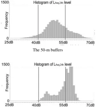
The histograms of the exposure assessments for the 50-m and the 400-m buffers, and the Δ400-50 exposure
assessments are presented in Figure 3. The Δ400-50 ranges between -9.4 dB and +22.3 dB, with a mean
variation of +3.9 dB. Two thirds of the buildings presented a Δ400-50 higher than |3 dB|: 56.5% over +3 dB
Table 1 - Average of noise exposure assessments (LAeq,24h (in dB))
according to the surface area of exposure techniques (n=10 825)
Address Points 6-m Façade 50-m Buffer 100-m Buffer 150-m Buffer 200-m Buffer 250-m Buffer 300-m Buffer 350-m Buffer 400-m Buffer Sampled surface Mean sampled surface (m²) 4 566 7, 833 31,375 70,624 125,581 196,247 282,618 384,700 502, 488 Mean noise modeled surface (m²)* 4 507 5,734 24,120 55,376 99,916 157,645 227,374 313,033 410,203 LAeq24H Mean 51.0 49.6 50.4 51.4 52.1 52.7 53.2 53.6 53.9 54.2 SD† 7.1 6.5 6.3 6.1 5.9 5.8 5.6 5.3 5.1 4.9 Min 25.0 24.7 25.6 27.6 30.7 32.7 34.6 36.0 37.1 39.2 Max 72.0 71.8 69.1 66.4 65.3 64.4 63.6 63.0 62.7 62.2 1st quartile 47.0 45.4 46.3 47.1 47.7 48.3 49.0 50.0 51.2 52.0 Median 51.0 49.4 50.0 50.9 52.1 53.3 54.3 55.1 55.5 55.6 3rd quartile 55.0 53.8 54.5 56.1 57.1 57.5 57.6 57.7 57.7 57.8
* Mean noise modeled surface = mean sampled surface - built surface in the sampled area. †Standard Deviation. (from (16)
)
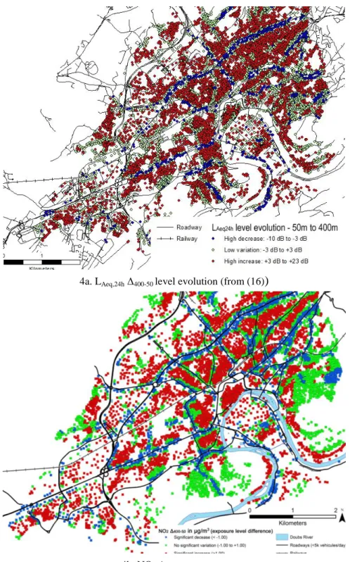
Not surprisingly, the spatial distributions buildings associated with highest 50 m exposure values (≥55 dB) were located along the main roadways. Conversely, when considering the 400-m indicator, this specific localization of buildings associated with the highest values along the main roadways is no longer observed, but spatial aggregates of medium noise exposition can be noted in the urban fringe. The spatial distributions of the Δ400-50 are presented in Figure 4a. The buildings associated to a Δ400-50 under -3 dB appeared to be
The 50-m buffers
The 400-m buffers
The Δ400-50 exposure assessment distribution
Figure 3 - The 50-m and the 400-m buffers, and the Δ400-50 exposure assessment distribution.
When the neighborhood surface increased, distance to the road, urban type and population density were significantly, positively and independently associated with the Δ400-50 noise level observed.
3.2 Air pollution
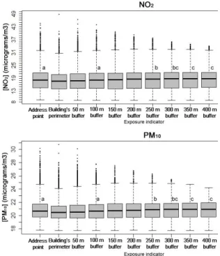
The air pollution levels were low for all pollutants and showed low heterogeneity both within samples and between samples (Figure 4). The NO2 values presented the highest heterogeneity (p<10
-3
). Pair wise comparisons of the ten means demonstrated the equivalency of the pollutant assessments. All of the 95% confidence intervals of the mean differences were totally included in the chosen zones of equivalence of [- 1.0 μg/m3; + 1.0 μg/m3].
4a. LAeq,24h Δ400-50 level evolution (from (16)
)
4b. NO2 Δ400-50 level evolution
Figure 4 - The LAeq,24h and NO2 Δ400-50 spatial distribution (from (13)).
Multivariate analysis conducted to the same results with the two air pollutants than with the noise exposure assessments. The spatial distributions of the Δ400-50 air pollutants were also comparable to
that of noise (Figure 4b), the buildings associated with a Δ400-50 under -1 μg/m 3
appeared to be localized very close to the main roadways.
Figure 4 - The ten noise exposure assessment distributions (average NO2 and PM10) (n=10 825) (from (13))
4. DISCUSSION
The recent development of powerful noise mapping softwares allows assessing the exposure to environmental noise at the scale of an agglomeration. However, the results highlight the real influence of the definition of the neighbourhood on the noise exposure assessment. When considering an increasing size of the considered space, the noise exposure assessment is increasing and the variability is decreasing. The impact identified on noise level was also identified on two air pollutants: NO2 and PM10.
Most studies of urban noise exposure attempt to highlight any impact on health and concentrate on high exposure levels (9, 17, 18), mainly near airports or roads with heavy traffic. However, our results demonstrate that a low proportion of facades were exposed to high noise levels. The city of Besançon did not contain an important airport or other particularly noisy infrastructure. The main noise source was ground transport, but no motorways crossed the inhabited districts. The results were observed in a medium-sized European city, which is defined by a population size between 100,000 and 500,000 inhabitants (19). Medium-sized cities are highly represented in terms of demography, accounting for more than 44 % of the European population (20). However, they tend to be less studied than the bigger cities (21, 22). Current efforts to consistently lower legal threshold limit values should lead major cities’ air pollution levels to decline to the levels currently observed in medium-sized cities. This makes today’s medium-sized cities of the highest importance for today and future public health studies.
5. CONCLUSIONS
Understanding the actual exposure of urban citizens is one of the biggest challenges of the next decade. Depending on the observation scale, the definition of the living neighborhood has a varying influence on the assessed exposure. These results applied to noise and air pollution environmental exposure assessment.
ACKNOWLEDGEMENTS
The authors would like to thank the city services, the urban community of Besançon (CAGB), the Besançon Urban Development Agency (AUDAB) and the Departemental Public Works Directorate (DDE) for their technical support. Quentin Tenailleau was a Ph.D. student supported by a grant from the city of Besançon.
REFERENCES
1. Belojevic G, Jakovljevic B, Stojanov V, Paunovic K, Ilic J. Urban road-traffic noise and blood pressure and heart rate in preschool children. Environment International 2008;34:226-231. doi:16/j.envint.2007.08.003
2. Miedema HM, Vos H. Exposure-response relationships for transportation noise. J. Acoust. Soc. Am 1998;104:3432-3445.
3. Muzet A. Environmental noise, sleep and health. Sleep Medicine Reviews 2007;11:135-142. doi:16/j.smrv.2006.09.001
4. Passchier-Vermeer W, Passchier WF. Noise exposure and public health. Environ Health Perspect 2000;108:123-131.
5. Babisch W. Guest Editorial: Noise and Health. Environ Health Perspect 2005;113:A14-A15.
6. Clark C, Martin R, van Kempen E, Alfred T, Head J, Davies HW, et al. Exposure-effect relations between aircraft and road traffic noise exposure at school and reading comprehension: the RANCH project. Am. J. Epidemiol 2006;163:27-37. doi:10.1093/aje/kwj001
7. de Kluizenaar Y, Gansevoort RT, Miedema HME, de Jong PE. Hypertension and road traffic noise exposure. J. Occup. Environ. Med 2007;49:484-492. doi:10.1097/JOM.0b013e318058a9ff
8. Murphy E, King EA, Rice HJ. Estimating human exposure to transport noise in central Dublin, Ireland. Environment International 2009;35:298-302. doi:16/j.envint.2008.07.026
9. Matsui T, Stansfeld S, Haines M, Head J. Children’s cognition and aircraft noise exposure at home--the West London Schools Study. Noise Health 2004;7:49-58.
10. Hong J, Kim J, Lim C, Kim K, Lee S. The effects of long-term exposure to railway and road traffic noise on subjective sleep disturbance. J. Acoust. Soc. Am 2010;128:2829-2835. doi:10.1121/1.3493437 11. National Institute of the Statistics and the Economic Studies, 2009. Results of the Population Census -
2009 [WWW Document]. URL http://www.recensement.insee.fr/basesInfracommunales.action (accessed 11.1.13).
12. Pujol, S., Houot, H., Antoni, J. P. & Mauny, F. Linking traffic and noise models to explore spatio-temporal distribution of noise pollution: an example in Besançon (France). in Int. Inst. Acoust. Vib. (2012)
13. Tenailleau QM, Mauny F, Joly D, François S, Bernard N. Air pollution in moderately polluted urban areas: How does the definition of "neighborhood" impact exposure assessment? Environ Pollut. 2015 ;11;206:437-448.
14. EMEP/EEA, 2009. EMEP/EEA air pollutant emission inventory guidebook 2009. Technical guidance to prepare national emission inventories. European Monitoring and Evaluation Programme & European Environment Agency, Luxemburg (Luxemburg).
15. Cambridge Environmental Research Consultants, 2014. ADMS-Urban presentation [WWW Document]. ADMS-Urban Present. URL http://www.cerc.co.uk/environmental-software/ADMS-Urban-model.html (accessed 10.9.14).
16. Tenailleau QM, Bernard N, Pujol S, Houot H, Joly D, Mauny F. Assessing residential exposure to urban noise using environmental models: does the size of the local living neighborhood matter? J Expo Sci Environ Epidemiol. 2015;25(1):89-96.
17. Stansfeld S, Berglund B, Clark C, Lopez-Barrio I, Fischer P, Öhrström E, et al. Aircraft and road traffic noise and children’s cognition and health: a cross-national study. The Lancet 2005;365:1942-1949. doi:16/S0140-6736(05)66660-3
18. Babisch W, Neuhauser H, Thamm M, Seiwert M. Blood pressure of 8-14 year old children in relation to traffic noise at home--results of the German Environmental Survey for Children (GerES IV). Sci. Total Environ 2009;407:5839-5843.
19. Bobby 1999 Boddy, M., 1999. Geographical economics and urban competitiveness: a critique. Urban Stud. 36, 811–842.
20. Giffinger, R., Fertner, C., Kramar, H., Meijers, E., 2007. City-ranking of European medium-sized cities. Cent. Reg. Sci. Vienna UT.
21. Ehrlich, P.R., Holdren, J.P., 1974. Human Population and the Global Environment: Population growth, rising per capita material consumption, and disruptive technologies have made civilization a global ecological force. Am. Sci. 62, 282–292.
22. Selden, T.M., Song, D., 1994. Environmental Quality and Development: Is There a Kuznets Curve for Air Pollution Emissions? J. Environ. Econ. Manag. 27, 147 – 162.