Assessing Dunnett and MCP-Mod based approaches in
two-stage dose-finding trials
Évaluation des approches basées sur le test de Dunnett et
MCP-Mod dans des essais de détermination de dose en deux
étapes
Jihane AOUNI1,2, Jean Noel BACRO2, Gwladys TOULEMONDE2,3, Pierre COLIN1, Loic DARCHY1and Bernard SEBASTIEN1
1Sanofi, Research and Development, 91385 Chilly-Mazarin, France, jihane.aouni@sanofi.com 2IMAG, Univ Montpellier, CNRS, Montpellier, France
3Lemon, INRIA
RÉSUMÉ. Identifier la bonne dose ou la dose optimale est l’une des difficultés majeures rencontrées lors du développe-ment d’un médicadéveloppe-ment. Par conséquent, l’étude dédiée à la détermination de la dose est une étape clé dans le dévelop-pement du médicament et des progrès méthodologiques relatifs à l’analyse de ces études ont été accomplis récemment, en mettant davantage l’accent sur l’identification du profil dose-réponse de l’efficacité. L’étude de détermination de dose avec un design fixe, placebo-contrôlée, en groupe parallèles est toujours la norme, mais les essais adaptatifs présentent, dans certains cas, de plus en plus d’intérêt. Le but de cet article est de revoir les méthodologies les plus récentes pour les essais adaptatifs de détermination de dose : ces méthodes sont applicables dans les cas où une ou plusieurs doses sont abandonnées après l’analyse intermédiaire, ou encore lorsque seule la répartition des patients est modifiée après l’analyse intermédiaire. Cette revue est complétée par des simulations illustrant ces méthodologies, y compris une version en deux étapes de la méthode MCP-Mod proposée par les auteurs.
ABSTRACT. Identifying the right, or the optimal, dose is one of the major difficulty during drug development. As a consequence, the dedicated dose-finding study is a key milestone in the drug development and recent methodological progress has been made for the analysis of those studies, in putting more emphasis on the identification of the efficacy dose-response profile. The placebo controlled, parallel group, fixed design is still a standard for the dose-finding studies, but adaptive designs are becoming more attractive in some cirumstances. The aim of this paper is to review the most recent methodologies for adaptive dose-finding trials : those methods are applicable in the cases when one or several doses are dropped after the interim analysis as well when only the patient allocation is modified after the interim analysis. This review is complemented by simulations illustrating the methodologies, including a two-stage version of the MCP-Mod method proposed by the authors.
MOTS-CLÉS. Essais adaptatifs, Optimisation du design, Sélection de dose, Dunnett, MCP-Mod, Tests multiples, Deux étapes.
KEYWORDS. Adaptive trials, Design optimization, Dose selection, Dunnett, MCP-Mod, Multiple testing, Two-stage.
1. Introduction
It is generally accepted (Sacks et al. 2014), that the dose-finding methodology is a key factor of success or failure in the phase III and later phases of the drug development. Consequently the dose-finding stu-dies play a major role in drug development, these stustu-dies should be rigorously and efficiently designed. Apart from the oncology indications, in most cases, traditional dose-finding methodologies were essen-tially driven by multiple testing procedures : the highest well tolerated dose amongst those significantly (in using a suitable multiple testing procedure that controls the global type I error) superior to the control, with respect to the efficacy criterion in the dose-finding phase II study, was selected for later phases. As the need for more sound and informative approaches became more clear, more recent approaches moved the methodology from the multiple testing methods to the "modeling" based methods with the MCP-Mod (Mutiple Comparison Procedure and Modeling) approach (Bretz et al. 2005). Now current trend, in this
same spirit, is clearly to consider the dose selection as a statistical estimation problem and not anymore as a multiple testing problem.
In the following subsection, we will describe the methodologies related to both traditional and recent approaches in the analysis of dose-finding trials as well as the methodology related to adaptive designs, in particular the two-stage combination test. Section 2 is dedicated to the application of two-stage adap-tive designs to dose-finding trials ; we particularly propose a two-stage version of the MCP-Mod method. In Section 3, simulation study examples are conducted, under several dose-response scenarios, in order to assess operating characteristics of two-stage designs, based on multiple testing or MCP-Mod, and to evaluate the gain offered by deviating from the classical balanced randomization scheme.
1.1. Methodology for dose-finding trials
Multiple testing approach
Multiple testing procedures were traditionnaly considered in dose-finding studies when the primary objective was to conclude whether one, or possibly more than one, dose was significantly superior than the control (placebo) with respect to the primary efficacy criterion. In this context, the main concern is the control (if possible in its strong sense1) of the type I error. A large number of multiple comparison procedures are available : we can mention Bonferroni (Henning and Westfall 2015), closed testing pro-cedures like Hommel (Hommel 1988) and Hochberg (Hochberg 1988), and Dunnett (Dunnett 1955). We briefly present the last two approaches.
Closed testing procedure The closed testing procedure (Henning and Westfall 2015) are now amongst the most popular approaches for multiple comparisons. It can be described as follows :
let µk = Ek(Y ) be the expectation of the variable Y in dose arm k (with k = 0 representing the placebo
group) ; we can form the K elementary hypotheses of interest : H0,1 : µ1 = µ0, ..., H0,K : µK = µ0
(i) then all possible set of intersection of hypotheses are built : for each v ⊆ {1, ..., K} we define H0v = ∩j∈vH0,j,
(ii) for each intersection test a local α-level test is built
(iii) and then an elementary hypothesis H0,iis rejected if all the intersection tests H0v that contain H0,i
are rejected at α level.
It can be shown that this procedure controls the type I error in the strong sense. In practice, the popular Hommel (Hommel 1988) or Hochberg (Hochberg 1988) methods (widely used for dose-finding studies as well) are examples of closed testing procedures (Henning and Westfall 2015).
Dunnett procedure The classical "Dunnett’s test" (Dunnett 1955) is a multiple comparison proce-dure used to compare each of several treatments with a single control. It consists on conducting Student’s t-statistic successively to every treatment/experimental group compared to a single control group and then to compute simultaneous confidence intervals for the contrasts µk − µ0, taking into account of the
correlation between the ( ¯Yk − ¯Y0)k terms (through the common term ¯Y0), where ¯Yk is the average
res-ponse within dose arm k. For the following, we will assume without loss of generality that the common standard deviation of the response Y is σ = 1, we will note n the common sample size within each dose arm, Zk = 1 √ 2 ¯ Yk− ¯Y0
p1/n the standardized mean treatment difference for any arm k.
Concretely a dose (from dose arm k for instance) is considered as significantly superior to placebo if ¯
Yk− ¯Y0 ≥ ˆσdK,α where dK,αis a constant that depends on the number of doses, K, and the α level. It is
also possible to derive an adjusted global p-value for the testing that there is at least one dose superior to placebo. Calling H0K the hypothesis, µi = µ0, ∀i ≤ K, the test p-value is
p = PHK 0 (maxk≤KZk ≥ maxk≤Kz obs k ) = 1 − PHK 0 (maxk≤KZk ≤ maxk≤Kz obs k ) = 1 − P (∀k ≤ K, Zk ≤ max k≤Kz obs k )
Under H0K, and for any number B, we have : P (∀k ≤ K : Zk ≤ B) = E[P (∀k ≤ K : Zk ≤ B| ¯ Y0 p1/n)] = E[P(∀k ≤ K, ¯Yk r 1 n ≤ √ 2B + ¯Y0 r 1 n| ¯ Y0 p1/n)] = E[ Q k≤K P (∀k ≤ K, ¯Yk r 1 n ≤ √ 2B + ¯Y0 r 1 n| ¯ Y0
p1/n)] (since all ¯Yk are independent) = R [Φ(x)( Q k≤K (1 − Φ(√2B + x)))] dx (since ¯Yk r 1 n ∼ N (0, 1) and ¯Y0 r 1 n ∼ N (0, 1)) 2 = R [Φ(x)((1 − Φ(√2B + x)))K] dx. Finally we obtain, p = Z [Φ(x)(Y k≤K (1 − Φ(√2max k≤KZ obs k + x)))] dx = Z [Φ(x)((1 − Φ(√2max k≤KZ obs k + x))) K] dx
It is important to notice that there is another "standard" (as opposed to the Adaptive Dunnett’s test that we will present in the next sections) version of Dunnett’s test, sometimes called the step-down Dunnett’s test. This version of the test uses the closed testing procedure associated to the following local tests : H0v, v ⊆ {1, ..., K} defined by µi = µ0, ∀i ∈ v are rejected if maxi∈vY¯i− ¯Y0 ≥ ˆσd|v|,α where |v| is
the number of elements in v. Because the constants d|v|,α are ≤ dK,α (the constant for the usual test), we
can conclude that this step-down version is slightly more powerful than the standard one. Using exactly the same calculations as above, we can deduce p-values for the local tests of the step-down version : pv = R [Φ(x)((1 − Φ( √ 2max k∈v Z obs k + x)))|v|] dx
Dose-response modeling approach : MCP-Mod
The MCP-Mod procedure (Bretz et al. 2005) is a new methodology for analyzing the dose-finding stu-dies that has an increasing popularity. It involves two steps : MCP and Mod steps respectively. The first step, MCP, is associated to the evidence of a drug effect over the doses (strictly speaking, when a signi-ficant dose-response signal for the clinical endpoint is noticed) using a predefined set of M candidate models (Emax, linear, exponential, etc...). Optimal linear contrasts of dose group means are computed for each candidate dose-response models3. A multiple comparison procedure is applied, controlling the alpha level for the family of null hypotheses associated with the contrasts. The idea behind this method is to compute a threshold dM so that PH0[max
m≤M
c0mµˆ σ [(c0mµ)ˆ
≥ dM] = α, where ˆµ = (ˆµ1, ..., ˆµK)0 is the
vec-tor of empirical mean responses in dose arms, cm is the optimal linear contrast associated to the model
m, m = 1, ..., M (c0m, like for all matrices in the following, represents the transpose of cm), and H0 is
the set of null hypotheses corresponding to all the contrasts c1, ..., cM; then we accept models where
c0mµˆ σ [(c0mµ)ˆ
≥ dM.
Note that this test satisfies the closed testing principle since dv ≤ dM when v is a subset of {1, ..., M }.
Therefore, by tabulating the law of Zv = max
m∈v
c0mµˆ σ \(c0mµ)ˆ
, we seek the threshold dv such that PHv 0 =
(max
m∈v
c0mµˆ σ [(c0mµ)ˆ
≥ dv) = α and we reject H0vif max m∈v
c0mµˆ σ \(c0mµ)ˆ
≥ dv, where H0v is the set of null hypotheses
corresponding to the contrasts cm, for m ∈ v.
After detecting a dose-response signal, the process is continued and advanced to the next step, the Mod step. This latter step is dedicated to the search of the Minimal Effective Dose or doses that achieve a targetted fraction of the maximal drug effect
All MCP-Mod applications presented later in this article were implemented using the MCP-Mod R pa-ckage developed in (Bornkamp et al. 2009).
1.2. Two-stage adaptive design
The two-stage procedure is a general testing procedure that enables to combine the results of two inde-pendent tests, summarized by their p-values, in a global test which, based on a particular combination of the two p-values, enables to control the type I error at any pre-specified level. The procedure, presented in details in (Bauer and Kieser 1999), is briefly described in the following.
In order to reject H0v one must do :
1. a local test of H0v with the stage 1 analysis which gives us pv1 2. a local test of H0v with the stage 2 analysis which gives us pv2
3. a combined/global test (i.e. "Two-stage procedure") by using the inverse normal combination function defined as follows :
pv∗ = C(pv1, pv2) = 1 − Φ(w1Φ−1(1 − p1v) + w2Φ−1(1 − pv2)), where w12+ w22 = 1.
Under H0v, we have w1Φ−1(1 − pv1) + w2Φ−1(1 − pv2) ∼ N (0, w12+ w22 = 1).
Then, H0v is rejected if pv∗ ≤ α.
Combining different phases in the development of medical treatments within a single trial was discussed in (Bauer and Kieser 1999). In their paper, the authors explained the general two-stage procedure, as well as the procedure when assuming an order relation among the parameters. They also presented a simulation study with different scenarios and computed the relative power for global hypothesis for each proposed scenario. They finally discussed the sample size reassessment.
In (Vandemeulebroecke 2006), the author proposes a general framework for two-stage tests that encom-passes the combination test mentionned above, and provides a link with the conditional error function approach, including the adaptive Dunnett test which is described thereafter.
2. Two-stage adaptive design applied to dose-finding trials
We will now focus on the cases when the dose-finding studies are adaptive. We will essentially cover the following situations :
(i) the sponsor might choose a seamless phase II/phase III design for operational reasons : at interim analysis some doses are dropped and the remaining one(s) is used for the phase III part of the trial (ii) the sponsor might be obliged to drop some doses at interim analysis for safety reasons or futility
(unethical to keep patients at doses that clearly show no efficacy)
(iii) the sponsor might decide to perform an interim analysis and then modify the design (modify patient allocation to doses) in order to optimize it.
For the first two situations only non-model based methods are appropriate (because if only 1 or 2 doses are available at second stage, it is not possible to estimate dose effect models at stage 2). For this purpose we will present some methods inherited from Dunnett’s test. For the third situation, we will consider some methods based on MCP-Mod approach.
2.1. Non dose-response model based two-stage
Two-stage Dunnett Combination test
As already explained in the previous section, the idea is to locally test H0v hypothesis, at a level α, and a Dunnett test is commonly applied. Let pvi be the adjusted p-value of the standard Dunnett test, where i is the index representing each stage (stage 1 and stage 2), i.e. i = {1, 2}. In order to reject H0v we must perform :
1. a local Dunnett test of H0v with the stage 1 analysis which gives us pv1 2. a local Dunnett test of H0v with the stage 2 analysis which gives us pv2
3. a global Dunnett test by using the inverse normal combination function defined in the previous section
Adaptive Dunnett test
The adaptive Dunnett procedure as presented in (Koenig et al. 2008), is based on the closed test prin-ciple and the conditional error function approach suggested in (Müller and Schäfer 2001). This approach can be summmarized as follows : in order to test any single hypothesis H in an adaptive way, we can first define a function A from the sample space of the first stage denoted by X1, to [0, 1], so that
EH(A(X1)) ≤ α (A(.) is called the conditional error function). Then, by using any test based on the
data of the second stage only resulting in a p-value, named q, we can define a global test that rejects hypothesis H whenever q ≤ A(X1) : this procedure controls the type I error.
This approach is generalized in (Müller and Schäfer 2001), in order to allow that the second stage ana-lysis involves the first stage data as well, provided that the sample size, n is fixed. Starting from any test ϕ, (ϕ = 1 means reject H), in defining the conditional error function, A(X1) = EH(ϕ = 1|X1), we can
define a global test if, for any p-value, q (q is p-value if q has, under H, a uniform distribution over [0, 1]), we have : q ≤ A(X1) = EH(ϕ = 1|X1). An important feature of this approach is that the original test ϕ
can be applied if no adaptations are performed.
This approach is applied using the Dunnetts’ test and the closed test principle in (Koenig et al. 2008) in order to define the adaptive Dunnett test. The derivation of the adaptive Dunnett test is summarized the-reafter : the aim is to test local hypotheses H0v where v ⊆ {1, ..., K}. The same notations as in Section 1.1 are used : Zk represents the standardized mean difference vs placebo and Z
(1)
k , Z
(2)
k represent the
same quantity but with only the data from the first stage and second stage respectively.
Stage 1 Conditional error function
The stage 1 conditional error function is defined by Av(X1) = PHv
0(ϕv = 1|X1), where X1 represents the stage one data and ϕv represents the global test (with data of stage 1 and stage 2). Therefore, we can
write PHv
0(ϕv = 1|X1) = PH0v(max
k∈v Zk ≥ dv|X1).
Using the same notations and methods as for the derivation of the global Dunnett p-value above, it is shown in (Koenig et al. 2008) that Av(X1) = 1 −R Φ(x)( Q
k∈v (1 − Φ(√2 √ ndv − √ n1Z (1) k √ n − n1 + x))) dx. Starting from this conditional error function, as detailed in (Koenig et al. 2008), there are two possibili-ties for the second stage p-values : they are described thereafter.
Separate stage 2 Dunnett p-value
In this approach, the second test only involves the data from the second stage. We can derive the p-value of the Dunnett test for the data of the second stage only, knowing that some doses could have been dropped : qvS = PHv
0( maxk∈v∩F 2
Zk(2) ≥ max
k∈v∩F2
Zk(2),obs), then qvS = 1 − R Φ(x)((1 − Φ(√2 max
k∈v∩F2
Zk(2),obs + x)))|v∩F2|dx where F 2 is the set of retained doses at stage 2. By application of the method, the final test associated to hypothesis H0v is signiticant if qvS ≤ Av(X1), see (Koenig et al. 2008).
Conditional stage 2 Dunnett p-value
It is defined by qvC = PHv 0( maxk∈v∩F 2 Zk ≥ max k∈v∩F2 Zkobs|X1). It is equal to : qCv = 1 −R Φ(x)( Q k∈v∩F2 (1 − Φ(√2 √ n max k∈v∩F2 Zkobs −√n1Z (1) k √ n − n1 + x))) dx.
The global test is significant if qvC ≤ Av(X1). An important property shown in (Koenig et al. 2008) is
that if the local hypothesis tested, H0v, only involves doses retained in second stage then the conditionnal Stage 2 Dunnett test corresponds to the standard Dunnett test. This property is not verified by the Sepa-rate two-stage version.
Then the closed testing procedure is applied : to test the global hypothesis that at least one dose is superior to placebo then the method is applied to the local test H0v with v = {1, ..., K} ; and to test whether a particular dose dk is superior to placebo the method is applied to all local tests H0v, v ⊆ {1, ..., K}, such
that k ∈ v.
Properties and practical implementation In (Koenig et al. 2008), properties and practical imple-mentation of the adaptive Dunnett’s test has been also assessed, through simulations. For this purpose the authors simulated various scenarios of dose adaptation, and compared the adaptive Dunnets’s procedure (the conditional second stage version), the two-stage Dunnett’s procedure with combination test and the "classical" Dunnett’s test (but in its step-down version). From those simulations, involving two doses and a placebo, the authors concluded to the superiority of the adaptive Dunnett test :
(i) in case of no adaptation, the adaptive Dunnett (which is equivalent, in its conditional stage two version, to the standard Dunnett) is superior to the two-stage combination Dunnett test.
(ii) when the adaptation consists in dropping the dose with lowest observed mean at interim analysis, then adaptive Dunnett is only slightly superior to two-stage combination Dunnett (they are almost equivalent), and both are superior to the "standard" step-down Dunnett.
(iii) when adaptation does not depend on efficacy (mimicking situations when drop of dose is induced by safety reasons) then adaptive Dunnett is slightly superior to two-stage combination Dunnett and both are generally superior to the "standard" step-down Dunnett.
2.2. Two-stage MCP-Mod
We describe here a new application of the two-stage combination test, that we propose, as described in Section 1.2, to MCP-Mod procedure, for dose-finding trials. If we define local hypotheses H0v defined by subset of the list of candidate dose-response models, we can perform a combined two-stage test as follows. If pvi is now the adjusted p-value of the MCP-Mod test, and to reject H0v, we must perform :
1. a local MCP-Mod test of H0v with the stage 1 analysis which gives us pv1 2. a local MCP-Mod test of H0v with the stage 2 analysis which gives us pv2
3. a combined MCP-Mod test by using the inverse normal combination function previously defined Then, H0v is rejected if pv∗ ≤ α.
To globally test if there is at least one "significant" dose-response model, the test proposed above is performed with v being the whole set of dose-response models.
2.3. Design optimization
In this section, we will discuss design optimality issues with the objective to assess how interim analysis can be used to optimize the design. There are several definitions and approaches for design optimization : we will use the Bayesian Optimal Design approach of (Miller et al. 2007).
Bayesian Optimal Design for dose-finding studies
The Bayesian optimality criterion proposed in (Miller et al. 2007) can be described as follows :
(i) A parametric dose-response model is chosen : we have chosen the Sigmoid-Emax model that assi-gns to a dose x, the mean dose-response f (x, θ) = E0+
Emaxxα
EDα50+ xα, θ = (E0, Emax, ED50, α) 0.
(ii) A set of scenarios is defined : to each of it a specific parameter value θscenario is chosen as well as
a prior probability πscenario, that the corresponds to the prior belief in the scenario.
(iii) The efficiency of the design at a given dose x is derived from the asymptotic variance of the contrast vs placebo (computed using the delta-method).
It is proportional to the quantity called d(x, design, θ) = (g(x, θ) − g(0, θ))0M−1(g(x, θ) − g(0, θ)), where g(x, θ) = ∂f (x, θ) ∂θ and M (design, θ) = P kwkg(xk, θ) 0g(x k, θ) is the Fisher
information matrix and wk is the percentage of patients assigned to dose arm k. The efficiency of
the design at dose x is the inverse of this quantity : 1/d(x, design, θ).
(iv) Now if we do not limit to a single dose, but we want to assess the efficiency over a range of doses [xδ, xmax], where xδ that gives a mean difference of δ versus placebo (the dose such that
f (xδ) − f (0) = δ) ; then, it is defined as : Φc(design, θ) = (
Rxmax
xδ d(x, design, θ) dx)
−1.
We define the relative efficiency of an arbitrary design with respect to the balanced design by Ef fc(design, θ) = Φc(design, θ)/Φc(balanced, θ).
(v) Using the various scenarios and their prior beliefs, we can define the efficiency of the design : Ψ(design) = P
jπjEf fc(design, scenario = θj),
where Ef fc(design, scenario = θj) =
(Rxmax xδ,j d(x, design, θj) dx) −1 (Rxmax xδ,j d(x, balanced, θj) dx)−1 .
Application of two-stage design optimization : re-allocation of patients
Adaptive designs have always been essentially used in the last two decades, in order to select doses, or more precisely to drop doses that appear unsafe or unefficient. Recently, these designs were used in a different context, which is the optimization of stage 2 by optimizing patients allocation, see (MacCal-lum and Bornkamp 2015), (Geiger et al. 2012, (Christen et al. 2004) and (Grieve 2017). More precisely, adaptation may also turn into a modification of the dose allocation ratio putting more emphasis on the most promising doses or even increasing sample size to tentatively rescue a poorly responsive trial. We will now focus on this same problem of optimization of a the second stage of the design using the tools and methodologies above described.
Adaptive Bayesian optimal design
In the following, we present the calculations shown in (Miller et al. 2007), but assuming, to simplify, that there is no delay between the conduct of the interim analysis and the enrollment of the patients for stage 2 (and then no enrollment during the conduct of the analysis itself). The optimization of the second stage of the design is conducted as follows.
Let n(1)i be the number of patients for the dose diat stage 1, the first step consists in up-dating the prior
be-liefs, πj, of the scenarios θj; to do this, it is first assumed that the responses are normally distributed, then
for each dose, the observations means ¯Y0(1), ..., ¯YK(1)are independent, and ¯Yi(1) ∼ N (f (xi),
σ2
n(1)i ). We are interested in ¯Yi(1) − ¯Y0(1), the differences between observations means for each dose and placebo. These differences have a multivariate normal distribution, N (µ, σ2Σ), where µ = (f (x1) − f (x0), ..., f (xK) −
f (x0))0, i = 1, ..., K. Hence, the covariance matrix is :
Σ = 1/n(1)0 + 1/n(1)1 1/n(1)0 · · · 1/n(1)0 1/n(1)0 1/n(1)0 + 1/n(1)2 1/n(1)0 .. . . .. 1/n(1)0 · · · 1/n(1)0 1/n(1)0 + 1/n(1)K
Let’s denote hj, the density of this multivariate distribution for Scenario θj, the updated probabilities can
be calculated conforming to the following : πj,updated = πj.hj( ¯Y (1) 1 − ¯Y (1) 0 , ..., ¯Y (1) K − ¯Y (1) 0 )/[ Pnb of scenarios t=1 πt.ht( ¯Y (1) 1 − ¯Y (1) 0 , ..., ¯Y (1) K − ¯Y (1) 0 )],
where πj, πj,updated are respectively the prior and posterior probabilities for Scenario θj.
Then optimal design for the second stage are determined in optimizing : Ψ(design) =P
jπj,updatedEf fc(design, scenario = θj).
In concrete terms, the weights defining the design for the second stage can be optimized in two different ways :
(i) either the final analysis includes the data of the interim analysis also, like in (Miller et al. 2007) : then the new weights are constrained by wi ≥ w
(1)
i = n
(1)
i /ntotal and the number of patients to
enroll in second stage is n(2)i = wi.ntotal − n (1) i
(ii) or the final analysis does not mix the interim analysis data and the second stage data (like in two-stage testing) then the optimization in the weights wiis unconstrained and n
(2)
i = wi(ntotal−n (1) total).
3. Simulations
We complemented this review of methodology by simulations illustrating the application of the me-thods above described. Two sets of simulations were conducted :
(i) The first objective was to compare two-stage Dunnett testing with two-stage MCP-Mod testing. For Dunnett test we focused on the two-stage combination test, instead of the adaptive Dunnett test, to allow an easier comparison with MCP-Mod two-stage.
(ii) The second objective was to assess the efficiency of the optimal design approach (both adaptive and non adaptive).
In those simulations, the objective is to test that there is at least one dose superior than placebo, for Dunnett’s test (i.e. the local hypothesis Hv concerns the whole set of doses {d1, ..., dK}, and at least one
model associated with a "significant" dose-response for MCP-Mod (corresponds to the MCP step)). In the simulations below the combined two-stage test is performed using the weights w1 = w2 =p1/2.
3.1. Simulation study : comparison of MCP-Mod versus Dunnett approach
In this set of simulations, we simulated 10000 studies with the following design : – Five Doses=(0,0.25,0.5,0.75,1)
– N = 30 patients per dose
– For all scenarios, the variability is set to σ2 = 1
– The doses are to be compared to placebo (Dose=0) with one sided test at level α = 0.025
The five following methods will be compared : Dunnett global test, MCP-Mod global test, the two-stage Dunnett test and the two-two-stage MCP-Mod test that we propose. The power of each method will be estimated by :
\
power = #successf ul studies
#studies , for each scenario.
Five scenarios are considered : for all of them, the maximum effect is equal to 1, and the highest dose has always the highest effect ; they are explicited thereafter :
– Scenario 1 : linear response, mean response by dose=(0,0.25,0.5,0.75,1)
– Scenario 2 : linear delayed response, first 2 doses have no efficacy, then linear increase, mean res-ponse by dose=(0,0,0,0.5,1)
– Scenario 3 : ’flat’, all doses have the same efficacy, mean response by dose=(0,1,1,1,1)
– Scenario 4 : ’plateau’, linear start, then last 2 doses have the same efficacy, mean response by dose=(0,0.33,0.67,1,1)
– Scenario 5 : ’extreme’, only last dose shows efficacy, mean response by dose=(0,0,0,0,1)
For the global and the two-stage Dunnett, we used the ’asd’ R package, see (Parsons 2016). For global and two-stage MCP-Mod, we used the global MCP-Mod function of the ’MCPMod’ R package4, see (Bornkamp et al. 2017).
Results
In Table 3.1, power is given for each test (Dunnett global test, MCP-Mod global test, two-stage Dun-nett test and two-stage MCP-Mod test), estimated by the percentage of studies having a p-value ≤ 0.05.
4. to compute the guesstimates (i.e. MCP-Mod assumptions), it is assumed that dose 1 reaches 90% of the maximal effect, and dose 0.25 reaches 25% of the maximal effect
− Dunnett global test MCP-Mod global test two-stage Dunnett two-stage MCP-Mod Scenario 1 0.95 0.99 0.93 0.99 Scenario 2 0.92 0.98 0.89 0.98 Scenario 3 0.99 1 0.99 1 Scenario 4 0.98 1 0.97 1 Scenario 5 0.92 0.90 0.87 0.88
Tableau 3.1.:Power comparison of global Dunnett, global MCP-Mod, two-stage Dunnett and two-stage MCP-Mod, for the five chosen scenarios, Scenario 1 to Scenario 5
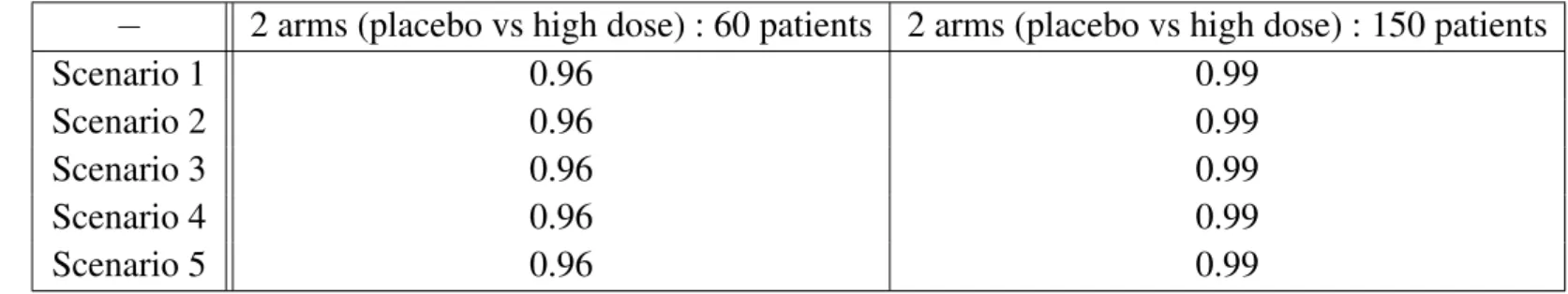
In Table 3.2, the student test power of the highest dose versus placebo is given, for 30 patients and 75 patients per arm respectively.
− 2 arms (placebo vs high dose) : 60 patients 2 arms (placebo vs high dose) : 150 patients
Scenario 1 0.96 0.99
Scenario 2 0.96 0.99
Scenario 3 0.96 0.99
Scenario 4 0.96 0.99
Scenario 5 0.96 0.99
Tableau 3.2.:Student test power comparison, for the five chosen scenarios, Scenario 1 to Scenario 5
We can notice from the simulations (Tables 3.1 and 3.2) that :
– The two-stage procedures are less powerful than their corresponding single testing procedures – The MPC-Mod procedure is superior than Dunnett’s procedure, both two-stage and global tests,
except for Scenario 5 ; for this latter scenario this might due to the fact that this efficacy profile could not be reproduced in any of the dose-response functions we considered in MCP-Mod (Emax and logistic) ; to fix such a problem, one can enrich the MCP-Mod family of functions with a Sigmoid-Emax function : this is what we have done for the simulations presented in the next sections
– For a total fixed number of patients, the most powerful test is to compare the highest dose versus placebo (75 patients per group with a student test (see Table 3.2)).
Globally, we conclude that two-stage testing without any adaptation is not useful and that MCP-Mod procedure is generally superior than Dunnett’s in both single stage and two-stage versions.
3.2. Optimal Bayesian design simulations
We will now assess, through simulations, how Bayesian optimal designs can improve the performance of the methods presented, in particular to which extent optimal patients re-allocation can improve the performance of the two-stage testing procedures.
Simulated Design
We simulated 1000 studies with the following design : – Five Doses=(0,0.25,0.5,0.75,1)
– N = 16 patients per dose
– For all scenarios, the variability is set to σ2 = 1
– The doses are to be compared to placebo (Dose=0) with one sided test at level α = 0.025
For comparison purpose, we also simulated 1000 studies with a total of 80 patients, with the patients allocation weights derived from optimal design computation.
Simulated Scenarios
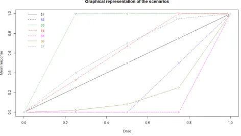
We simulated seven scenarios :
– Scenario 1 : linear response, mean response by dose=(0,0.25,0.5,0.75,1)
– Scenario 2 : linear delayed response, first 2 doses have no efficacy, then linear increase, mean res-ponse by dose=(0,0,0,0.5,1)
– Scenario 3 : ’flat’, all doses have the same efficacy, mean response by dose=(0,1,1,1,1)
– Scenario 4 : ’plateau’, linear start, then last 2 doses have the same efficacy, mean response by dose=(0,0.33,0.67,1,1)
– Scenario 5 : ’extreme’, only last dose shows efficacy, mean response by dose=(0,0,0,0,1)
– Scenario 6 : ’Exponential type’, slow efficacy then fast efficacy for high doses, mean response by dose=(0,0.02,0.08,0.25,1)
– Scenario 7 : ’Emax type’, fast efficacy then progressive plateau, mean response by dose=(0,0.4,0.70,0.95,1)
These scenarios are graphically presented in Figure 1. In this figure, Scenario i is denoted by Si, 1 ≤ i ≤ 7.
Optimal Design computation
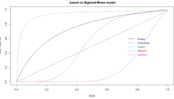
Table 3.3 summarizes the five chosen scenarios for the Sigmoid-Emax model, followed by their corres-ponding dose-response curves (Figure 2), that were used to compute the optimal design :
name parameter prior proba
Primary E0 = 0, Emax= 1.25, ED50 = 0.25, α = 1 π = 0.40
Quasi-linear E0 = 0, Emax = 48, ED50 = 48, α = 1 π = 0.15
Plateau E0 = 0, Emax = 1, ED50 = 0.015, α = 1 π = 0.15
Sigmoid-1 E0 = 0, Emax = 1.45, ED50 = 0.9, α = 8 π = 0.15
Sigmoid-2 E0 = 0, Emax = 1, ED50 = 0.45, α = 5 π = 0.15
Tableau 3.3.:Sigmoid-Emax parameter values, for the five chosen scenarios
Figure2.:Dose-response curves for the five chosen scenarios, based on Sigmoid-Emax model
Computational aspects To compute the optimal design, the δ value (the lowest difference of interest versus placebo) was set to 0.5 and we used ’optim’ function in R for the optimization part and we added a constraint : exclude the possibility of having no patients in stage 2 for a given dose. Concerning MCP-Mod, Sigmoid-Emax family was added to the set of candidate dose-response functions and to compute the guesstimates (i.e. MCP-Mod assumptions), it was assumed that 1 mg reaches 90% of maximal effect, and 0.25 mg reaches 25% of maximal effect.
Results
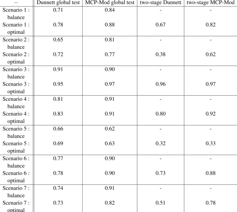
Table 3.4 shows the power of Dunnett global test, MCP-Mod global test, two-stage Dunnett test, and two-stage MCP-Mod test, based on the 7 scenarios described above, with 1000 studies simulated for each scenario, in the following three design versions :
– balanced design
– optimal design : the optimal weighs obtained were : w∗ = (0.308, 0.156, 0.299, 0.073, 0.163)0 – two-stage optimal design : 40 + 40 patients ; the design of the first part is the optimal design based on
prior beliefs (like above) and the design of the second part is based on the updated beliefs following the interim analysis
− Dunnett global test MCP-Mod global test two-stage Dunnett two-stage MCP-Mod Scenario 1 : balance 0.71 0.84 - -Scenario 1 : optimal 0.78 0.88 0.67 0.82 Scenario 2 : balance 0.65 0.81 - -Scenario 2 : optimal 0.72 0.77 0.38 0.62 Scenario 3 : balance 0.91 0.90 - -Scenario 3 : optimal 0.95 0.97 0.96 0.97 Scenario 4 : balance 0.81 0.91 - -Scenario 4 : optimal 0.83 0.91 0.80 0.92 Scenario 5 : balance 0.66 0.62 - -Scenario 5 : optimal 0.69 0.63 0.32 0.33 Scenario 6 : balance 0.77 0.90 - -Scenario 6 : optimal 0.78 0.90 0.73 0.88 Scenario 7 : balance 0.74 0.91 - -Scenario 7 : optimal 0.73 0.82 0.51 0.78
Tableau 3.4.:Power comparison of global Dunnett, global MCP-Mod, two-stage Dunnett and two-stage MCP-Mod, for the seven chosen scenarios, Scenario 1 to Scenario 7, three design versions : balanced, optimal and two-stage optimal designs
In general, as we have noticed in the previous simulations, MCP-Mod is superior than Dunnett : this was almost always true for the balanced design ; the two only exceptions were Scenario 3 and Scenario 5 which correspond to scenarios with lack of clear dose-response relationship (Scenario 3 : all doses are equally efficient, Scenario 5 : only last dose is efficient) ; this superiority of MPC-Mod over Dunnett applies for both balanced and optimal design.
The optimal design is superior to the balanced design in almost all cases, except for scenario 7 for both Dunnett MCP-Mod and for the second scenario, for MCP-Mod only.
Two-stage designs are generally inferior to the optimal design except for Scenario 3 and Scenario 4 for which the two-stage is slightly superior to the optimal design. For all other scenarios, the two-stage is inferior to the optimal design (two-stage is particularly bad for Scenario 2 and Scenario 5, cases when the optimal design does not perform well either) ; in fact when the performance of the optimal design is poor, the two-stage design does not correct enough. Bad performance of the two-stage design is pos-sibly due to the weight of stage 2 in the global test : it may be too small and the possibility to take w2 > w1 in the combination test should be considered. Also the weight of primary guess (π = 0.40) in
the computation of the optimal design could be too strong, and cannot be compensated by the evidence brought by 40 additional patients : maybe it could be worth considering equal weights in scenario to compute Bayesian efficiency. Also another possibility for improvement, for the two-stage MCP-Mod, that is worth considering for future research could be to modify the guesstimates (based on the interim analysis) when performing the second MCP-Mod analysis.
4. Discussion
In this paper we have reviewed various approaches for the design and analysis of adaptive dose-finding trials. Even though the placebo controlled, parallel group, fixed design is still a standard for the dose-finding studies, adaptive designs are more and more used. For the sponsor, design adaptation could be necessary, for ethical reasons for instance, or could be governed by the objective to gain knowledge at first step.
Our paper is mostly focused on the two-stage testing procedure, see (Bauer and Kieser 1999), that we applied to various methods of analysis of dose-finding trials : the traditional multiple testing approaches (those based on ANOVA and multiple testing), with a focus on Dunnett method, but also more recent "model-based" approaches in particular the MCP-Mod approach (Bretz et al. 2005).
We have also discussed the application of the two-stage design optimization in order to re-design stage 2, e.g. dose allocation ratio, choice of doses and/or sample size.
We conducted simulation studies in order to extensively assess some of the approaches proposed in the literature, as well as a new application of the two-stage combination test to the MCP-Mod procedure, that we proposed. Our simulation results showed that globally, MCP-Mod is better than Dunnett in terms of
power, optimal designs are better than balanced designs (for both testing procedures), but Dunnett/MCP-Mod two-stage design generally do not bring improvement as compared to optimal designs.
Our findings suggest improvements in the application of two-stage testing, especially in the context of MCP-Mod.
Bibliographie
Bauer, P. and Kieser, M. (1999). Combining different phases in the development of medical treatments within a single trial. Statistics in Medicine, 18(14) :1833–1848.
Bornkamp, B., Pinheiro, J., and Bretz, F. (2009). MCPMod : An R Package for the Design and Analysis of Dose-Finding Studies. Journal of Statistical Software, 29(7) :1–23.
Bornkamp, B., Pinheiro, J., and Bretz F. (2017). MCPMod : An R Package for the Design and Analysis of Dose-Finding Studies. R package version 1.0-10. https ://CRAN.R-project.org/package=MCPMod.
Bretz, F., Branson, M., and Pinheiro, J. (2005). Combining Multiple Comparisons and Modeling Techniques in Dose-Response Studies. Biometrics, 61(3) :738–748.
Christen, JA., Müller, P., Wathen, K., and Wolf, J. (2004). A bayesian randomized clinical trial : A decision theoretic sequential design. Canadian Journal of Statistics, 32(4) :387–402.
Dunnett, CW. (1955). A multiple comparison procedure for comparing several treatments with a control. Journal of the American Statistical Association, 50(272) :1096–1121.
Geiger, MJ., Skrivanek, Z., Gaydos, B., Chien, J., Berry, SM., Berry, D., and Anderson, JH. (2012). An Adaptive, Dose-Finding, Seamless Phase 2/3 Study of a Long-Acting Glucagon-Like Peptide-1 Analog (Dulaglutide) : Trial Design and Baseline Characteristics. Journal of Diabetes Science and Technology, 6(6) :1319–1327.
Grieve, AP. (2017). Response-adaptive clinical trials : case studies in the medical literature. Pharmaceutical Statistics, 16(1) :64–86.
Henning, KS. and Westfall, PH. (2015). Closed Testing in Pharmaceutical Research : Historical and Recent Developments. Statistics in biopharmaceutical research, 7(2) :126–147.
Hochberg, Y. (1988). A sharper Bonferroni procedure for multiple tests of significance. Biometrika, 75(4) :800–802. Hommel, G. (1988). A stagewise rejective multiple test procedure based on a modified Bonferroni test. Biometrika, 75(2) :383–386.
Koenig, F., Brannath, W., Bretz, F., and Posch, M. (2008). Adaptive Dunnett tests for treatment selection. Statistics in Medicine, 27(10) :1612–1625.
MacCallum, E. and Bornkamp, B. (2015). Accounting for parameter uncertainty in two-stage designs for Phase II dose-response studies. Modern Adaptive Randomized Clinical Trials : Statistical and Practical Aspects, pages 427–450. Miller, F., Guilbaud, O., and Dette, H. (2007). Optimal Designs for Estimating the Interesting Part of a Dose-Effect Curve. Journal of Biopharmaceutical Statistics, 17(6) :1097–1115.
Müller, HH. and Schäfer, H. (2001). Adaptive group sequential designs for clinical trials : combining the advantages of adaptive and of classical group sequential approaches. Biometrics, 57(3) :886–891.
Parsons, N. (2016). asd : Simulations for Adaptive Seamless Designs. R package version 2.2. https ://CRAN.R-project.org/package=asd.
Sacks, LV., Shamsuddin, HH., Yasinskaya, YI., Bouri, K., Lanthier, ML., and Sherman, RE. (2014). Scientific and regulatory reasons for delay and denial of FDA approval of initial applications for new drugs, 2000-2012. JAMA, 311(4) :378–384.