Dynamic calculation of a tapered shaft rotor made of composite material

(1)

http://www.techno-press.org/?journal=aas&subpage=7 ISSN: 2287-528X (Print), 2287-5271 (Online)

Dynamic calculation of a tapered shaft rotor made of

composite material

Zahi Rachid

1

, Refassi Kaddour

1a

_{and Habib Achache}

2b

1_{Laboratory of Mechanics of Structures and Solids LMSS, University of Sidi Bel Abbes, Algeria} 2_{University Dr Yahia Fares Médéa, Algérie}

(Received June 24, 2017, Revised September 6, 2017, Accepted September 9, 2017)

Abstract. This work proposes a theoretical and numerical study on the behavior of a tapered shaft rotor made of

composite materials by the classical version h and the version p of the finite element method. Hierarchical form functions are used to define the model. The purpose of this paper is to determine the expressions of the kinetic and potential energies of the tree necessary for the results of the equations of motion. A comparison between the version h and the p version of the finite element method of the functions of polynomial and trigonometric hierarchical forms with six degrees of freedom per node, of a composite tapered and cylindrical shaft which rotates at a constant speed about its axis. It is found that when the number of functions of form (the version p) is increased, the solution converges. It is also observed that the conicity of the shaft increases the rigidity with respect to a uniform shaft having the same mechanical properties. The numerical simulation allowed us to determine the natural frequencies and the critical speeds of the composite shaft systems are compared with those available in the literature and the effectiveness of the methods used are discussed.

Keywords: fibre composite multilayer plates; vibration; Structural mechanics; rotordynamics; dynamic

analysis

1. Introduction

The composite materials have opened up new avenues by increasing the performance of industrial machines (automotive, aerospace and aerospace sectors) thanks to their intrinsic qualities such as lightness (combined with high strength characteristics) corrosion. The field of use of machines has expanded through the development of new materials, developed from new design and manufacturing methods. The interest of composites for dynamic rotor applications has been demonstrated both numerically and experimentally, accompanied by the development of many new advanced composite materials. Cylindrical composite shafts have also been developed by researchers. Vibration analysis research projects using the hierarchical finite element method have proved that this method gives better accuracy in determining the eigenvalues of a composite tree with a constant section. Studies concerning the non-uniform rotation of composite structures, a

Corresponding author, Ph.D., E-mail: zahirachid72@yahoo.fr

a_Professor

(2)

work available from Bauchau on hollow shafts in which the optimization of the tapered wall thickness is treated using Rayleigh. A mechanical model was developed by w. Kim et al on composite cone shafts which runs at a constant speed around its axis, which are used the general method of Galerkin.

Several authors have focused their attention on the development of tapered shaft rotors. The work of Archer et al, presented a linearly tapered element based on Timoshenko's beam theory. They incorporated the shear effects into the formulation by defining the shear angle as an additional nodal variable, which leads to twelve degrees of freedom per element. Greenhill et al extended the approach by including all the intrinsic effects of the rotation system in a conic element, and developed closed-form expressions for elementary structural matrices.

More recently, Edney et al, proposed a tree compatible C1-type cone based on the formulation proposed by Archer. Assuming the constant shear distribution over the element length, they maintained only four degrees of freedom per node, the slope being incorporated throughout the entire rotation of the section.

The work of Gmur and Rodrigues relates to the development of the linearly cone-shaped element of the C0 type with a variable number of nodal points. Similar to the works of Edney et al the proposed elements have only four degrees of freedom per node. These being the transverse displacement and the total rotation of the section in the two orthogonal planes. They include the effects of translational inertia and rotation, gyroscopic moments, internal viscous and hysteretic damping, shear deformation, and mass eccentricity.

A model for linear vibration analysis of rotor developed by Genta et al has been described in works. This model is based on the finite element method (FEM) and includes a coherent matrix formulation for the axisymmetric constants of the beam.

The interest of composites for dynamic rotor applications has been demonstrated both numerically and experimentally, accompanied by the development of many new advanced composite materials. Cylindrical composite shafts have also been developed by researchers.

Kim et al used best theory to determine the critical speeds of a rotating shaft containing layered layers of composite materials; the tree was modeled as a Bresse-Timoshenko beam. Bert and Kim examined the dynamic instability of a transmission shaft in composite materials under the effect of twisting torsional coupling and Coriolis forces.

In the present work, the Timoshenko theory is adopted for a composite material shaft which rotates at a constant speed about its axis. The spatial solutions are obtained using the method of the finite elements version P. Numerical results are presented for a tapered steel shaft and hollow tapered shaft made of graphite/epoxy composite materials with boundary conditions free embedding and compare with that found in Literature. Another study using trigonometric and polynomial shape functions to determine the critical speeds of a tapered shaft in bore/epoxy module composite materials with the bi-supported boundary condition.

The work is devoted to determining dynamic characteristics such as natural frequencies and critical speeds and a comparison between a tapered shaft and results found for a dynamic system to a cylindrical shaft.

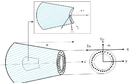
2. Cinematic equations

(3)

Fig. 1 transfer according to the orientation of the fibers and the angle α

This law, generally called the generalized Hooke law, introduces the symmetric stiffness matrix [C]. The elastic behavior of an orthotropic composite material in matrix form is given by Berthelot

et al. { 𝜎11 𝜎22 𝜎33 𝜏23 𝜏31 𝜏12} = [ 𝐶11 𝐶12 𝐶13 0 0 0 𝐶21 𝐶22 𝐶23 0 0 0 𝐶31 𝐶32 𝐶33 0 0 0 0 0 0 𝐶44 0 0 0 0 0 0 𝐶55 0 0 0 0 0 0 𝐶66]{ 𝜀11 𝜀22 𝜀33 𝛾23 𝛾31 𝛾12} (2)

The constraints in the reference base (1', 2’, and 3’) shown in Fig. 1 are

[𝜎] = [𝑄]{𝜀} (3)

Where

[Q] is the matrix of the stiffness coefficients related to the axes of the laminate (1', 2', 3'), and calculating the stresses [Tη] expressed as a function of the angle η called the orientation of the fibers given by Berthelot et al.

{ 𝜎𝑟𝑟 𝜎𝜃𝜃 𝜎𝑧𝑧 𝜏𝑟𝜃 𝜏𝑥𝑟 𝜏𝑥𝜃} = [ 𝑄11 𝑄21 𝑄31 0 0 𝑄61 𝑄12 𝑄22 𝑄32 0 0 𝑄62 𝑄13 𝑄23 𝑄33 0 0 𝑄63 0 0 0 𝑄44 𝑄54 0 0 0 0 𝑄45 𝑄55 0 𝑄16 𝑄26 𝑄36 0 0 𝑄66]{ 𝜀𝑟𝑟 𝜀𝜃𝜃 𝜀𝑧𝑧 𝛾𝑟𝜃 𝛾𝑥𝑟 𝛾𝑥𝜃} (4)

The second transfer is done using the matrix expressed as a function of the angle α of the conic in the frame, (e⃗⃗⃗ ,e_r ⃗⃗⃗⃗ ,k θ⃗⃗ ) The matrix of the stiffness coefficients [Kij] expressed as a function of

(4)

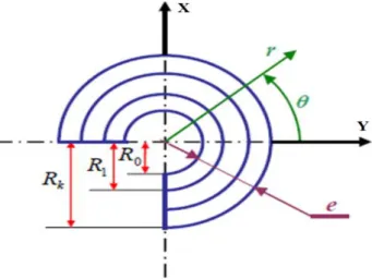
Fig. 2 Tree layers of composite materials [𝜎] = [𝐾𝑖𝑗]{𝜀} (5) { 𝜎𝑟𝑟 𝜎𝜃𝜃 𝜎𝑧𝑧 𝜏𝑟𝜃 𝜏𝑧𝑟 𝜏𝑧𝜃} = [ 𝐾11 𝐾21 𝐾31 𝐾41 𝐾51 𝐾61 𝐾12 𝐾22 𝐾32 𝐾42 𝐾52 𝐾62 𝐾13 𝐾23 𝐾33 𝐾43 𝐾53 𝐾63 𝐾14 𝐾24 𝐾34 𝐾44 𝐾54 𝐾64 𝐾15 𝐾25 𝐾35 𝐾45 𝐾55 𝐾65 𝐾16 𝐾26 𝐾36 𝐾45 𝐾56 𝐾66]{ 𝜀𝑟𝑟 𝜀𝜃𝜃 𝜀𝑧𝑧 𝛾𝑟𝜃 𝛾𝑧𝑟 𝛾𝑧𝜃} (6)

One notices in the case of a composite tapered shaft Kim stratified

𝜏𝑟𝜃= -𝜏𝑧𝜃tgα (7)

The aim of this work is to determine the equation of motion from kinetic energy and potential energy as well as the system stiffness matrix. The calculation is based on the development of Kim’s article. { 𝜎𝑧𝑧 𝜏ɵ𝑧 𝜏𝑧𝑟 } = [ 𝐾′33 𝐾′43 𝐾′53 𝑓. 𝐾′34 𝑓. 𝐾′44 𝑓. 𝐾′54 𝑓. 𝐾′35 𝑓. 𝐾′45 𝑓. 𝐾′55 ] { 𝜀𝑧𝑧 𝛾ɵ𝑧 𝛾𝑧𝑟 }+[ 𝐶′11 𝐶′21 𝐶′31 𝐶′12 𝐶′22 𝐶′32 ] {𝜎_𝜎𝜃 𝑟} (8)

3. Energy of deformation and kinetic of the tree

The Timoshenko model is adopted for transverse vibrations. It is assumed that the whole of the section perpendicular to the axis z remains plane after deformation.

The field of deformations writes 𝜀𝑧𝑧 =

𝜕𝑈𝑧

𝜕𝑧 + 𝑟 sin 𝜃 𝜕𝜓𝑦

(5)

𝛾𝑧𝜃 = 𝜓𝑥sin 𝜃 + 𝜓𝑌cos 𝜃 − sin 𝜃 𝜕𝑈𝑥 𝜕𝑥 + cos 𝜃 𝜕𝑈𝑦 𝜕𝑧 + 𝑟 𝜕∅ 𝜕𝑧 (10)

𝛾𝑧𝑟 = 𝜓𝑦sin 𝜃 − 𝜓𝑥cos 𝜃 + sin 𝜃

𝜕𝑈𝑦

𝜕𝑧 + cos 𝜃 𝜕𝑈𝑥

𝜕𝑧 (11)

The formula of the energy deformation (a single beam element) is Eda =1

2∫{𝜎𝑖𝑗}

𝑇

{𝜀𝑖𝑗}𝑑𝑉 (12)

That it can be written in the following form 𝐸𝑑𝑎 = 1 2 ∫ ∫ ∫ [ 𝐾′33 𝐾′ 43 𝐾′ 53 𝑓. 𝐾′34 𝑓. 𝐾′₄₄ 𝑓. 𝐾′ 54 𝑓. 𝐾′₃₅ 𝑓. 𝐾′45 𝑓. 𝐾′55 ] 𝑇 𝑅_𝑘 0 2𝜋 0 𝐿 0 ∗ [ 𝜕𝑈𝑧 𝜕𝑧 + 𝑟 sin 𝜃 𝜕𝜓𝑦 𝜕𝑧 − 𝑟 cos 𝜃 𝜕𝜓𝑥 𝜕𝑧 (𝜓𝑥sin 𝜃 + 𝜓𝑦cos 𝜃 − sin 𝜃

𝜕𝑈𝑥 𝜕𝑧 + cos 𝜃 𝜕𝑈𝑦 𝜕𝑧 + 𝑟 𝜕∅ 𝜕𝑧) (𝜓𝑦sin 𝜃 − 𝜓𝑥cos 𝜃 + sin 𝜃

𝜕𝑈𝑦 𝜕𝑧 + cos 𝜃 𝜕𝑈𝑥 𝜕𝑧) ] ∗ 𝑟𝑑𝑟𝑑𝜃 𝑑𝑧 (13)

Eq. (13) in the developed form takes the form The expression of the kinetic energy of the tree is

(14)

Given by the following equation 𝐸𝑑𝑎 =

1

2∫ 𝜌 (𝑅̇⃗ 𝑃 0⁄ . 𝑅̇⃗ 𝑃 0⁄ ) (15) The kinetic energy in the developed form is

𝐸𝑐𝑎 = 1 2∫ [𝐼𝑚(𝑈𝑥 2 ̇ + 𝑈_𝑦2̇ + 𝑈 𝑧2̇ ) + 𝐼𝑑(𝜓𝑥2̇ + 𝜓𝑦2̇ ) − 2𝛺𝐼𝑝𝜓𝑥𝜓𝑦̇ + 2𝛺𝐼𝑝𝜙̇ + 𝐼𝑝𝜙̇2+ 𝛺2𝐼𝑝 𝐿 0 + 𝛺2_𝐼 𝑑(𝜓𝑥2̇ + 𝜓𝑦2̇ )] 𝑑𝑧 (16)

(6)

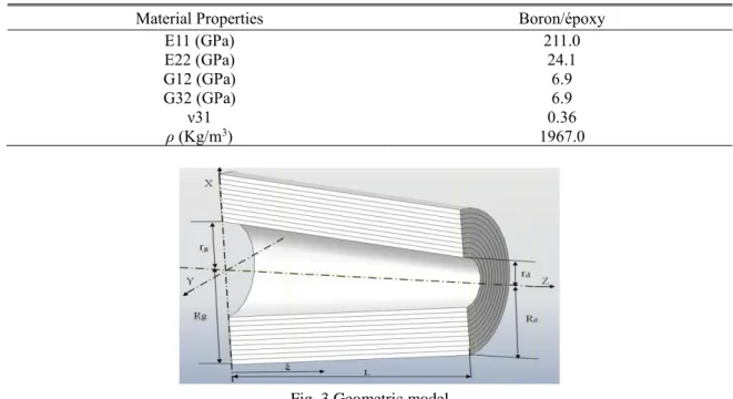
Table 1 Properties of composite material

Material Properties Boron/époxy

E11 (GPa) E22 (GPa) G12 (GPa) G32 (GPa) ν31 ρ (Kg/m3₎ 211.0 24.1 6.9 6.9 0.36 1967.0

Fig. 3 Geometric model

4. Defining the hierarchical finite element

In the hierarchical or polynomial finite element method, the error can be checked. It consists in varying the degree of interpolation of the elements while preserving the size of the elements and their degrees of interpolation. The passage from n to n+1 does not alter functions of form Ni (i = 1 ....n).

4.1 Polynomial of legendre

The Legendre polynomials Pi (z) defined between [-1; 1] are given by { 𝑃0(z) = 1 𝑃𝑛(𝑧) = 1 2𝑛 _𝑛! 𝑑𝑛 𝑑𝑧𝑛 [(𝑧2− 1)𝑛] 𝑛 = 1,2,3 … … … (17)

They are solutions of the following differential equation

(1 − z2_{)ÿ − 2zẏ + n(n + 1)y = 0 n = 1,2,3 … … . N} j (z) = √2j − 1 2 ∫ Pj−1(t)dt x −1 n = 1,2,3 … … .. It is possible to define a set of modes

In our calculation we have made a change of variable ξ such that ξ varies between [0; 1] ξ=z/L with (0 ≤ ξ ≤ 1)

(7)

5. Hierarchical tapered element

In our study, we used the method of finite hierarchical elements with polynomial form functions that possess certain orthogonality such as the Legendre polynomial [55]. The variable section tree is modeled by hierarchical 3D beam elements. Each element shown in Fig. 3.1 has two nodes 1 and 2. The true radius between r and R.

5.1 Geometric model

Our geometric model is a tapered shaft made of a boron/epoxy composite material, the properties of which are given in Table 1, of length L = 2.56 m. It consists of ten layers [90°, 45°, -45°, 0°, -45°, --45°, 90 °] with identical thicknesses equal to e = 5.4 cm. The outer diameter of one end is D1 = 12.8 cm.

In this paper, the rotating boron/epoxy shaft is modeled by a single element of length L, by two elements and at the end by three elements of the same lengths for a rotation speed of 400 rd/s.

The displacement field of a point of the beam is given by Ux= [NUx]{qUx} = ∑ xn p_Ux n=1 (t). N_n(ξ) Uy = [NUy] {qUy} = ∑ yn p_Uy n=1 (t). N_n(ξ) Uz = [NU_z]{qU_z} = ∑ Zn p_Uz n=1 (t). Nn(ξ) ψx= [Nψ_x]{qψ_x} = ∑ ψxn p_ψx n=1 (t). Nn(ξ) ψy= [N ψy] {q ψy} = ∑ ψyn p_ψ n=1 (t). N_n(ξ) ∅ = [N∅]{q∅} = ∑ ∅n p∅ n=1 (t). N_n(ξ) [N_k′_{] =}∂[Nk] ∂ξ , with ( k = Ux, Uy, Uz, ψx; ψy; ϕ)

From Eq. (13), we find the shape of the elementary stiffness matrix[K_ae_]

∂Eda ∂{qUz} = [1 L∫ A11[NUz ′_]T 1 0 [N_Uz′]dξ] {qU_z} + [ 1 L∫(1 + f)B12[N∅ ′_]T 1 0 [N_Uz′]dξ] {q∅} = [KUz]{qUz} + [K1]{q∅} (18)

(8)

(19) (20) ∂Eda ∂{qψx} = ([1 L∫ B11[Nψx ′ _]T 1 0 [Nψx ′ _{]dξ] + [L ∫ f. (A} 22+ A33)[Nψ_x] T 1 0 [Nψ_x]dξ] − ∫ (1 + f)B13[N_ψx′] T 1 0 [Nψx ′ _{]dξ ) {q} ψ_x} − [1 2L∫ (1 + f)B12[NUy ′_]T 1 0 [Nψy ′ _{] dξ] {q} Ux} + [∫ f. (A22+ A33) [N_Uy′] T 1 0 [Nψ_x]dξ − 1 2L∫ (1 + f)B13[Nψx ′_]T 1 0 [N_ψ′_x]dξ] {qU_y} + [1 2L∫ (1 + f)B12[NUy ′_]T 1 0 [N_ψ′_y] dξ] {qUx} + [∫ f. (A22+ A33) [N_Uy′] T 1 0 [Nψx]dξ − 1 2L∫ (1 + f)B13[Nψx ′_]T 1 0 [Nψ′_x]dξ] {qUy} + ([1 2∫ (1 + f)B12[Nψy] T 1 0 [Nψx ′ _]dξ] − [1 2∫ (1 + f)B12[Nψx] T 1 0 [Nψ′_y] dξ]) {qψy} (21)

(9)

𝜕𝐸𝑑𝑎 𝜕{𝑞𝜓𝑥} = [Kψx]{qψx} − [K2] T_{q Ux} + [K3+ K4] T_{q Uy} − [K5] {qψy} (22) ∂Eda ∂ {qψy} = ([1 L∫ B11[Nψy ′ _]T 1 0 [Nψy ′ _{] dξ] + [L ∫ f. (A} 22+ A33) [Nψ_y] T 1 0 [Nψ_y] dξ] − ∫(1 + f)B13[N_ψy′] T 1 0 [N_ψ′_y] dξ ) {qψy} − [1 2L∫(1 + f)B12[NUy ′_]T 1 0 [Nψy ′ _{] dξ] {q} Uy} + [∫ f. (A22+ A33) [N_Uy′] T 1 0 [Nψ_y] dξ − 1 2L∫(1 + f)B13[Nψy ′_]T 1 0 [Ny′]dξ] {qU_x} + ([1 2∫(1 + f)B12[Nψx] T 1 0 [Nψ′_y] dξ] − [1 2∫(1 + f)B12[Nψx] T 1 0 [Nψy ′ _{] dξ]) {q} ψ_x} = [KψY]{qψY} − [K2] T_{q Uy} + [K3+ K4] T_{q Ux} − [K5] T_{q ψx} (23) ∂Eda ∂{q∅}= [ 1 L∫ B22[N∅ ′_]T 1 0 [N∅ ′_{]dξ] {q} ∅} + [ 1 L∫ (1 + f)B12[NU ′_]T 1 0 [N∅ ′_{]dξ] {q} Uz} = [K∅]{q∅} + [K1]T{qU_z} (24) Where

Aij and Bij are given in the appendix. The kinetic energy in the developed form is

Eca=

1

2ImL ∫{qu̇x}T

1

0

[NUx]T[NUx]{qu̇x}dξ+ ∫{qu̇y} T 1 0 [NUy] T [NUy]{qu̇y}dξ + ∫{qu̇y} T 1 0 [NUy] T [NUy]{qu̇y}dξ + 1 2IdL [ ∫ {q̇_ψ x} T 1 0 [Nψ_x] T [Nψ_x] {q̇_ψ x} dξ + ∫ {q̇_ψ y} T 1 0 [Nψ_y] T [Nψ_y] {q̇_ψ y} dξ ] (25)

(10)

+ΩI_pL [∫[N∅] 1 0 {q̇_∅}dξ] +1 2IPL [∫{q̇_∅} T 1 0 [N_∅]T[N_∅]{q̇_∅}dξ] -ΩI_pL [∫{qψx} T 1 0 [Nψ_x] T [Nψ_y] {q̇ψ_y} dξ] + L 2Ω 2_I p

From the Lagrange equation we find the forms of the elementary matrices [M_ae_{] and [G} a e_] 𝑑 𝑑𝑡( 𝜕𝐸𝑐𝑎 𝜕{𝑞𝑢̇𝑥} ) − 𝜕𝐸𝑐𝑎 𝜕{𝑞𝑢𝑥} = [𝐼𝑚𝐿 ∫ [𝑁𝑢𝑥]𝑇[𝑁𝑢𝑥] 𝑑𝜉 1 0 ] {𝑞̈𝑢𝑥} = [𝑀𝑢𝑥]{𝑞𝑢̈𝑥} (26) 𝑑 𝑑𝑡( 𝜕𝐸𝑐𝑎 𝜕{𝑞𝑢̇𝑦} ) − 𝜕𝐸𝑐𝑎 𝜕{𝑞𝑢𝑦} = [𝐼𝑚𝐿 ∫ [𝑁𝑢𝑦] 𝑇 [𝑁𝑢𝑦] 𝑑𝜉 1 0 ] {𝑞̈𝑢𝑦} = [𝑀𝑢𝑥]{𝑞𝑢̈𝑥} (27) 𝑑 𝑑𝑡( 𝜕𝐸𝑐𝑎 𝜕{𝑞𝑢̇𝑧} ) − 𝜕𝐸𝑐𝑎 𝜕{𝑞𝑢𝑧} = [𝐼𝑚𝐿 ∫ [𝑁𝑢𝑧]𝑇[𝑁𝑢𝑧] 𝑑𝜉 1 0 ] {𝑞̈𝑢𝑧} = [𝑀𝑢𝑧]{𝑞𝑢̈𝑧} (28) 𝑑 𝑑𝑡( 𝜕𝐸𝑐𝑎 𝜕{𝑞̇𝜓_𝑥} ) − 𝜕𝐸𝑐𝑎 𝜕{𝑞𝜓_𝑥} = [𝐼𝑑𝐿 ∫ [𝑁𝜓𝑥] 𝑇 [𝑁𝜓𝑥] 𝑑𝜉 1 0 ] {𝑞̈𝜓𝑥} + [Ω𝐼𝑝𝐿 ∫ [𝑁𝜓𝑥] 𝑇 [𝑁𝜓𝑦] 𝑑𝜉 1 0 ] {𝑞̇𝜓𝑥} = [𝑀𝜓𝑥]{𝑞̈𝜓𝑥} + [𝐺1] 𝑇_{𝑞̇ 𝜓𝑦} (29) 𝑑 𝑑𝑡( 𝜕𝐸𝑐𝑎 𝜕 {𝑞̇𝜓𝑦} ) − 𝜕𝐸𝑐𝑎 𝜕 {𝑞𝜓𝑦} = [𝐼𝑑𝐿 ∫ [𝑁𝜓𝑦] 𝑇 [𝑁𝜓𝑦] 𝑑𝜉 1 0 ] {𝑞̈𝜓𝑦} + [Ω𝐼𝑝𝐿 ∫ [𝑁𝜓𝑦] 𝑇 [𝑁𝜓𝑥]𝑑𝜉 1 0 ] {𝑞̇𝜓𝑦} = [𝑀𝜓𝑦] {𝑞̈𝜓𝑦} + [𝐺1] 𝑇_{𝑞̇ 𝜓𝑥} (30) 𝑑 𝑑𝑡( 𝜕𝐸𝑐𝑎 𝜕{𝑞̇∅} ) − 𝜕𝐸𝑐𝑎 𝜕{𝑞∅} = [𝐼𝑑𝐿 ∫[𝑁∅]𝑇[𝑁∅] 𝑑𝜉 1 0 ] {𝑞̈∅} = [𝑀∅]{𝑞̈∅} (31) Where

𝜌: the density of the composite tree. Im: the moment of mass inertia

Ip : the moment of polar inertia

Id : the moment of diametrical inertia

(11)

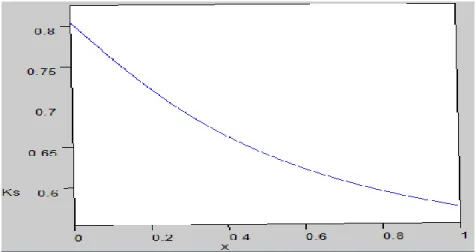
Fig. 4 Variation of Timoshenko shear coefficients as a function of r/R Table 2 Critical speed of boron/epoxy composite shaft

Investigators Critical speed Ωcr1 (tr/mn) Theories or Methods

Kim et Bert 5872 shell of Sanders

Chang et al. 5919 Beam of Bernoulli-Euler

Bert et Kim 5762 Beam of Timoshenko

Rimo sino 5767 SHBT (simplified Homogenized Beam Theory) without shearing effect

Zahi et al. 5790.4 Beam of Timoshenko with the p version

Id(ψẋ 2

+ ψẏ 2

): represents the effect of rotary inertia

Ω2Id(ψx2+ ψy2): represents the effect of centrifugal stiffening, is very small before Ω2Ip, It

will be neglected by the subsequent analysis. ImD ; IdD ; IpD Are defined in the appendix.

The equation of free vibration motion is given by Euler-Lagrange

[𝑀]{𝑞̈} + [[𝐺]]{𝑞̇} + [𝐾]{𝑞} = {0} (32)

6. Results and discussions

A program is developed for the calculation of the system’s own frequencies and critical speeds. The results obtained compared with those available in the literature show the speed of convergence by increasing the number of hierarchical form functions. A conical shaft boron epoxy is presented in this study with support-support boundary conditions, and a discussion is established to determine the influence of the various parameters (taper, number of trigonometric form functions, number of polynomial form functions and number of elements).

To determine the shear coefficient of Timoshenko ks, regardless of the section, the work cited in Kim’s paper was used.

(12)

𝑘𝑠=

6𝐸𝑧𝑧(1 − 𝑚̅4)(1 + 𝑚̅2)

𝐺𝑧𝑥𝜈𝑧𝑥(2𝑚̅6+ 18𝑚̅4− 18𝑚̅2− 2) − 𝐸𝑧𝑧(7𝑚̅6+ 27𝑚̅4− 27𝑚̅2− 7)

Where: m̅ =r/R.

The critical speed, cited in Table 2 and obtained by our model, converges to those found in the literature, for different theories and methods.

Case 2: r ≠ R (α ≠ 0)

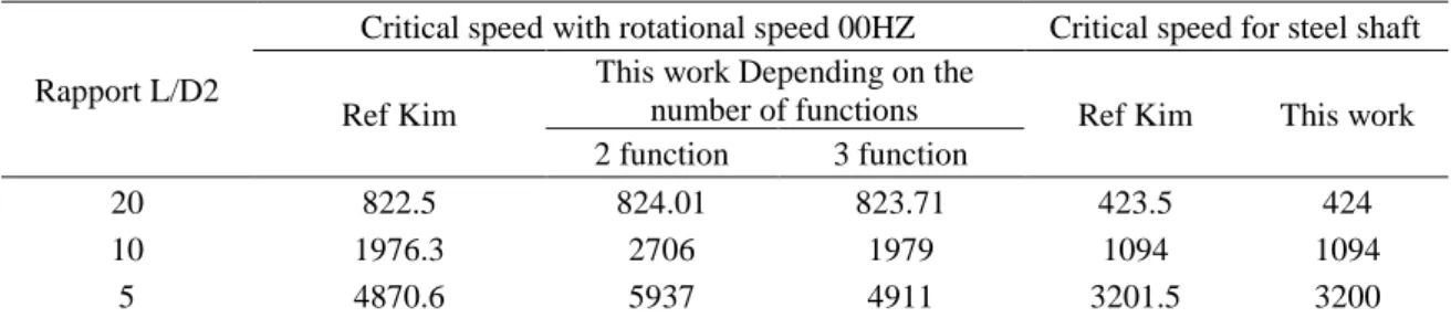
Table 3 Critical speed of the tapered shaft in composite materials

Rapport L/D2

Critical speed with rotational speed 00HZ Critical speed for steel shaft Ref Kim

This work Depending on the

number of functions Ref Kim This work 2 function 3 function

20 822.5 824.01 823.71 423.5 424

10 1976.3 2706 1979 1094 1094

5 4870.6 5937 4911 3201.5 3200

Table 3 shows the critical frequency of several shape functions for one shaft embedded at one end and free at the other end. We note that our results agree with those found by Kim for the different L

D2 ratios in both cases (tree made of graphite/epoxy composite materials with fiber

orientation (00) and homogeneous steel shaft). The properties of the composite material used are (Kim): α=1.7° Rg-rg=5.4 mm, rd=1 mm Rd=d2/2=6.4 mm; The speed of rotation 400 rad/s, Ezz=192 GPa, Gzx=4.07 GPa, γzx=0.24, Gxy=3 GPa ρ=1610 kg/m3_.

Table 4 Critical velocity of the cylindrical shaft for a single element and several hierarchical trigonometric form functions

c.l A-A Number of elements with (α=0)

Number of trigonometric functions

Critical speed with rotational speed 00 HZ

1 4 5821.68 5760

1 6 5796.6 5734.8

1 8 5792.4 5730.4

1 10 5791.2 5729.7

Table 5 Critical velocity of the cylindrical shaft for two elements and several hierarchical trigonometric form functions

c.l A-A Number of elements with (α=0)

2 4 6420 6360

2 6 5910 5848.2

2 8 5829 5760

(13)

Table 6 Critical velocity of the cylindrical shaft for three elements and several trigonometric hierarchical form functions

Critical speed with rotational speed 400 HZ 3 4 6420 6360 3 6 5910 5848.2 3 8 5829 5760 3 10 5808 5745 1 2 3 5800 5900 6000 6100 6200 6300 6400 6500 Critical sp ee d Nbr of elément 4 foctions 6 foctions 8 foctions 10 foctions

Fig. 5 of the citric velocity as a function of the number of trigonometric hierarchical form functions of a double-supported cylindrical shaft (A-A)

The variation of the critical velocity as a function of the number of trigonometric hierarchical form functions of a bi-supported cylindrical shaft (A-A) is shown in Fig. 5. We note that the increase of the functions of trigonometric forms (the version p of the finite elements) leads to the exact solution, without increasing the number of elements.

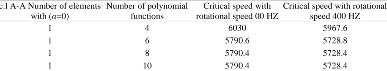
Table 7 Critical velocity of the cylindrical shaft for a single element and several polynomial hierarchical form functions

Number of polynomial functions

1 4 6030 5967.6

1 6 5790.6 5728.8

1 8 5790.4 5728.4

(14)

Table 8 Critical speed of the cylindrical shaft for two elements and several polynomial hierarchical form functions c.l A-A Number of elements with (α=0) Number of polynomial functions

2 4 5794.2 5732

2 6 5790.6 5728.8

2 8 5790.6 5728.8

2 10 5790.6 5728.8

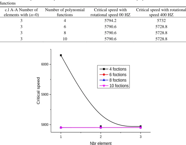
Table 9 Critical speed of the cylindrical shaft for three elements and several polynomial hierarchical form functions

c.l A-A Number of elements with (α=0)

Critical speed with rotational speed 400 HZ 3 4 5794.2 5732 3 6 5790.6 5728.8 3 8 5790.6 5728.8 3 10 5790.6 5728.8 1 2 3 5800 5900 6000 4 foctions 6 foctions 8 foctions 10 foctions Critical sp ee d Nbr element

Fig. 6 Variation of the citric velocities as a function of the number of polynomial hierarchical form functions of a bi-supported cylindrical shaft (A-A)

Fig. 7 illustrates the variation of the critical speed as a function of the number of polynomial hierarchical form functions of a bi-supported cylindrical shaft. The results obtained show that whatever the increase in the number of elements or the number of functions of polynomial forms, the solution converges to the exact solution. We note that the use of polynomial hierarchical form functions gives good results by contributing to the functions of trigonometric hierarchical forms.

(15)

Table 10 Critical speed of the tapered shaft for a single element and several functions of hierarchical form trigonometric

c.l A-A Number of elements

with (α=1.7rad) Nbr of function trigo

1 4 9360 9180

1 6 9013.8 8866.2

1 8 8992.6 8655.4

Table 11 Critical speed of the tapered shaft for two element and several functions of hierarchical form trigonometric

2 4 9208.2 9013.8

2 6 9107.8 8951.2

2 8 9046.4 8822.4

Table 12 Critical speed of the tapered shaft for three element and several functions of hierarchical form trigonometric

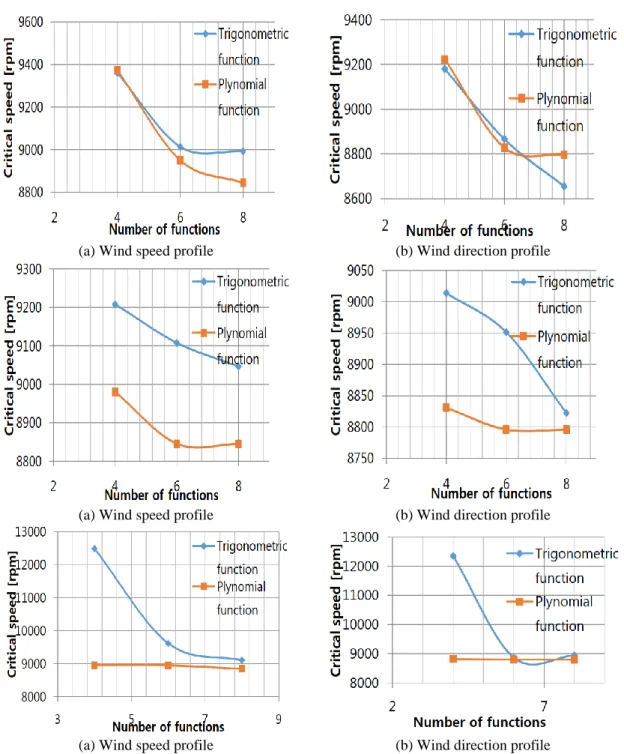
Critical speed with rotational speed 400 HZ 3 4 12490.8 12343.8 3 6 9617.4 8866.2 3 8 9102.4 8942.4 1 2 3 9000 9500 10000 10500 11000 11500 12000 12500 13000 4 foctions 6 foctions 8 foctions Critical sp ee d Nbr of element 1 2 3 8500 9000 9500 10000 10500 11000 11500 12000 12500 4 foctions 6 foctions 8 foctions Critical sp ee d Nbr of element

(a) Wind speed profile (b) Wind direction profile

Fig. 7 Variation of the citric velocity as a function of the number of trigonometric hierarchical form functions of a bi-supported tapered shaft (A-A)

Fig. 8 illustrates the variation of the four critical speeds as a function of the number of trigonometric functions of a bi-supported shaft (A-A) for a rotation speed equal to 0 rpm and 400 rpm. We note that the results converge towards the exact solution without increasing the numbers of the elements.

(16)

Table 13 Critical velocity of the cone tree for a single element and several polynomial hierarchical form functions c.l A-A Number of elements with (α=1.7rad) Number of polynomial functions

1 4 9373.8 9222.6

1 6 8950.2 8827.8

1 8 8844.8 8796

Table 14 Critical velocity of the cone tree for two elements and several polynomial hierarchical form functions

c.l A-A

Number of elements with (α=1.7rad)

2 4 8980.2 8830.8

2 6 8844.8 8796

2 8 8844.8 8796

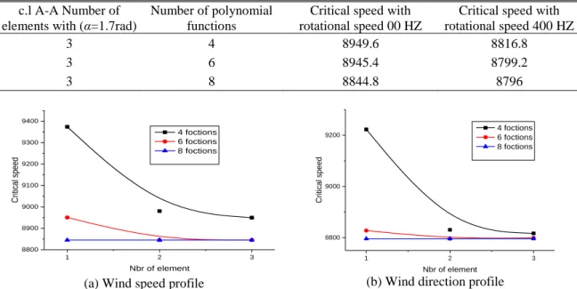
Table 15 Critical velocity of the cone tree for three elements and several polynomial hierarchical form functions

c.l A-A Number of elements with (α=1.7rad)

Critical speed with rotational speed 400 HZ 3 4 8949.6 8816.8 3 6 8945.4 8799.2 3 8 8844.8 8796 1 2 3 8800 8900 9000 9100 9200 9300 9400 4 foctions 6 foctions 8 foctions Critical sp ee d Nbr of element 1 2 3 8800 9000 9200 4 foctions 6 foctions 8 foctions Critical sp ee d Nbr of element

Fig. 8 Variation of the citric velocity as a function of the number of functions of polynomial hierarchical form of a bi-supported tapered shaft (A-A)

Fig. 9 shows the variation of the critical speeds as a function of the number of shape functions of a bi-supported shaft (A-A) for a rotation speed equal to 0 rpm and 400 rpm. We note that the results converge towards the exact solution. Note that the increase in the number of functions of polynomial hierarchical forms does not affect convergence.

(17)

Fig. 9 Convergence of the frequencies as a function of the number of hierarchical form functions of a bi-supported tree (A-A)

From the results obtained in Tables 13, 14 and 15, we notice that, regardless of the version used (class h, version p or version hp) of the finite elements, using the functions of polynomial forms, the convergent results to the exact solution. It is noted that the increase of the values of the natural

(18)

frequencies and the critical speeds of the conical shaft imply the increasing rigidity of the conical shaft under the same conditions.

7. Conclusions

This work presents a comparative study of two finite elements modeling of polynomial and trigonometric conic shapes of rotors and those relating to the conventional cylindrical approach. The results of numerical simulations are analyzed using the p version as well as the conventional version h of the finite element method. These are validated by the results obtained in the literature. Comparisons between numerical simulations show that using the p version of the polynomial conic finite elements allows very good predictions on the dynamic behavior of composite cone shaft rotors compared to the two other versions h and h-p. The modeling by polynomial tapered elements shows a high accuracy of the results. The increase in the values of the natural frequencies and the critical speeds of the conical shaft imply the increasing stiffness of the conical shaft

References

Archer, J.S. (1965), “Consistent matrix formulation for structural analysis using finite element techniques”, J. Struct. Div., 1910-1918.

Bauchau, O.A. (1983), “Optimal design of high speed rotating graphite/epoxy shafts”, J. Compos. Mater., 17, 170-181.

Bert, C.W. and Kim, C.D. (1995), “Whirling of composite-material driveshafts including bending, twisting coupling and transverse shear deformation”, J. Vibr. Acoust., 117, 17-21.

Berthelot, J.M. (1996), Matériaux Composites, Comportement Mécanique et Analyse des Structures, Deuxième Edition, Masson, Paris, France.

Chang, C.Y. (2004), “Vibration analysis of rotating composite shafts containing randomly oriented reinforcements”, Compos. Struct., 63, 21-32.

Cowper, G.R. (1966), “The shear coe$cient in Timoshenko’s beam theory”, J. Appl. Mech., 33, 335-340. Dharmarajan, S. and Mccutchen Jr, H. (1973), “Shear coe$cients for orthotropic beams”, J. Compos.

Mater., 7, 530-535.

Düster, A. and Rank, E. (2001), “The p-version of the finite element method compared to an adaptive h-version for the deformation theory of plasticity”, Comput. Meth. Appl. Mech. Eng., 190, 1925-1935. Edney, S.L., Fox, C.H.J. and Williams, E.J. (1989), “Finite element analyses of tapered rotors”, Proceedings

of the 7th International Modal Analysis Conference, Las Vegas, U.S.A.

Edney, S.L., Fox, C.H.J. and Williams, E.J. (1990), “Finite element analyses of tapered rotors”, J. Sound Vibr., 463-481.

Genta, G. and Gugliotta, A. (1984), Un Modello Per Studio Dinamico Dei VII Congres Naz AIMETA. Gmür, T.C. and Rodrigues, J.F. “A shaft finite element for rotors dynamics analysis”, J. Sound Vibr.

Greenhill, L.M., Bickford, W.B. and Nelson, H.D. (1985), “A conical beam finite element for rotor dynamics analysis”, J. Sound Vibr., 421-430.

Houmat, A. (2001), “A sector fourier p-element applied to free vibration analysis of sector plates”, J. Sound Vibr., 243, 269-282.

Kim, C.D. and Bert, C.W. (1993), “Critical speed analysis of laminated composite, hollow drive shafts”, Compos. Eng., 3, 633-643.

(19)

125-147.

Meirovitch, L. and Baruh, H. (1983), “On the inclusion principle for the hierarchical finite element method”, J. Numer. Meth. Eng., 19, 281-291.

Thomas, D.L. (1973), Wilson J. Sound Vibr., 31-315-330. EC

(20)

Appendix

MATRIX COEFFICIENTS, Kij

k11=q11*sa^4+2*(q13+2*q55)*sa^2*ca^2+q33*ca^4 k12=q12*sa^2+q23*ca^2 k13=q13*(sa^4+ca^4)+(q11+q33-4*q55)*sa^2*ca^2 k14=q36*ca^3+(q16-2*q45)*sa^2*ca k15=-(q13-q33+2*q55)*sa*ca^3-(q11-q13-2*q55)*sa^3*ca k16=-q16*sa^3-(q36+2*q45)*sa*ca^2 k22=q22 k23=q12*ca^2+q23*sa^2 k24=q26*ca k25=(q23-q12)*sa*ca k26=-q26*sa k33=q11*ca^4+2*(q13+2*q55)*sa^2*ca^2+q33*sa^4 k34=q16*ca^3+(q36+2*q45)*sa^2*ca k35= -(q13-q33+2*q55)*sa^3*ca-(q11-q13-2*q55)*sa*ca^3 k36=-q36*sa^3-(q16-2*q45)*sa*ca^2 k44=q44*sa^2+q66*ca^2 k45=-q45*sa^3-(q16-q36-q45)*sa*ca^2 k46=(q44-q66)*sa*ca k55=(q11+q33-2*q13-2*q55)*sa^2*ca^2+q55*(sa^4+ca^4) k56=q45*ca^3+(q16-q36-q45)*sa^2*ca k66=q44*ca^2+q66*sa^2 Were: q11=c11*cb^4+2*(c12+2*c66)*sb^2*cb^2+c22*sb^2 q12=(c11+c22-4*c66)*sb^2*cb^2+c12*(sb^4+cb^4) q13=c13*cb^2+c23*sb^2 q16=(c11-c12-2*c66)*sb*cb^3+(c12-c22+2*c66)*sb^3*cb q22=c11*sb^4+2*(c12+2*c66)*sb^2*cb^2+c22*cb^2 q23= c13*sb^2+c23*cb^2 q26=(c11-c12-2*c66)*sb^3*cb+(c12-c22+2*c66)*sb*cb^3 q33=c33 q36=(c13-c23)*sb*cb q44=c44*cb^2+c55*sb^2 q45=(c55-c44)*sb*cb q55=c44*sb^2+c55*cb^2 q66=(c11+c22-2*c12-2*c66)*sb^2*cb^2+c66*(sb^4+cb^4) 𝐴11= 2𝜋 ∑ 𝐾11 ∫ 𝑟𝑑𝑟 𝑅2𝑍 𝑅1𝑍 𝑘 𝑛=1 𝐴12= 𝜋 ∑ 𝐾12∫ 𝑟2𝑑𝑟 𝑅2𝑍 𝑅1𝑍 𝑘 𝑛=1

(21)

𝐴22= 𝜋 ∑ 𝐾22 ∫ 𝑟𝑑𝑟 𝑅2𝑍 𝑅1𝑍 𝑘 𝑛=1 𝐴33= 𝜋 ∑ 𝐾33∫ 𝑟𝑑𝑟 𝑅2𝑍 𝑅1𝑍 𝑘 𝑛=1 𝐵11 = 𝜋 ∑ 𝐾11∫ 𝑟3𝑑𝑟 𝑅2𝑍 𝑅1𝑍 𝑘 𝑛=1 𝐵12= 2𝜋 ∑ 𝐾12 ∫ 𝑟2𝑑𝑟 𝑅2𝑍 𝑅1𝑍 𝑘 𝑛=1 𝐵22= 2𝜋 ∑ 𝐾22 ∫ 𝑟3𝑑𝑟 𝑅2𝑍 𝑅1𝑍 𝑘 𝑛=1 𝐵13 = 𝜋 ∑ 𝐾13∫ 𝑟2𝑑𝑟 𝑅2𝑍 𝑅1𝑍 𝑘 𝑛=1 𝐼𝑚 = 2𝜋𝜌 ∑ ∫ 𝑟𝑑𝑟 𝑅2𝑧 𝑅1𝑧 𝑛=𝑘 𝑛=1 𝐼𝑑= 𝜋𝜌 ∑ ∫ 𝑟3 𝑅2𝑧 𝑅1𝑧 𝑑𝑟 𝑛=𝑘 𝑛=1 𝐼𝑝= 2𝜋𝜌 ∑ ∫ 𝑟3 𝑅2𝑧 𝑅1𝑧 𝑑𝑟 𝑛=𝑘 𝑛=1 [𝐾] = [ [𝐾𝑈_𝑍] 0 0 0 0 [𝐾₁]𝑇 0 [𝐾𝑈𝑌] 0 [𝐾₂+ 𝐾3]𝑇 [𝐾₄]𝑇 0 0 0 [𝐾𝑈𝑋] [𝐾₄]𝑇 [𝐾₆+ 𝐾7]𝑇 0 0 [𝐾₂+ 𝐾3] [𝐾5] [𝐾𝜓𝑌] [𝐾8]𝑇 0 0 [𝐾₄] [𝐾₆+ 𝐾7] [𝐾₈] [𝐾𝜓𝑥] 0 [𝐾₁] 0 0 0 0 [𝐾_∅_]] [𝑀] = [ [𝑀𝑈_𝑍] 0 0 0 0 0 0 [𝑀𝑈_𝑌] 0 0 0 0 0 0 [𝑀𝑈𝑋] 0 0 0 0 0 0 [𝑀𝜓𝑌] 0 0 0 0 0 0 [𝑀𝜓_𝑥] 0 0 0 0 0 0 [𝑀_∅]] [𝐺] = [ 0 0 0 0 0 0 0 0 0 0 0 0 0 0 0 0 0 0 0 0 0 0 −[𝐺1]𝑇 0 0 0 0 [𝐺₁] 0 0 0 0 0 0 0 0]