Statistics and Machine Learning in Python

(1)

HAL Id: hal-03038776

https://hal.archives-ouvertes.fr/hal-03038776v2

Submitted on 18 Dec 2020

HAL is a multi-disciplinary open access archive for the deposit and dissemination of sci-entific research documents, whether they are pub-lished or not. The documents may come from teaching and research institutions in France or abroad, or from public or private research centers.

L’archive ouverte pluridisciplinaire HAL, est destinée au dépôt et à la diffusion de documents scientifiques de niveau recherche, publiés ou non, émanant des établissements d’enseignement et de recherche français ou étrangers, des laboratoires publics ou privés.

Edouard Duchesnay, Tommy Lofstedt, Feki Younes

To cite this version:

Edouard Duchesnay, Tommy Lofstedt, Feki Younes. Statistics and Machine Learning in Python. Engineering school. France. 2020. �hal-03038776v2�

(2)

Python

Release 0.5

Edouard Duchesnay, Tommy Löfstedt, Feki Younes

(3)

(4)

1 Introduction 1

1.1 Python ecosystem for data-science . . . 1

1.2 Introduction to Machine Learning . . . 6

1.3 Data analysis methodology . . . 7

2 Python language 9 2.1 Import libraries . . . 9

2.2 Basic operations . . . 9

2.3 Data types . . . 10

2.4 Execution control statements . . . 17

2.5 List comprehensions, iterators, etc. . . 18

2.6 Functions . . . 21

2.7 Regular expression . . . 22

2.8 System programming . . . 23

2.9 Scripts and argument parsing . . . 29

2.10 Networking . . . 30

2.11 Modules and packages. . . 31

2.12 Object Oriented Programming (OOP) . . . 32

2.13 Style guide for Python programming . . . 33

2.14 Documenting . . . 33

2.15 Exercises . . . 35

3 Scientific Python 37 3.1 Numpy: arrays and matrices . . . 37

3.2 Pandas: data manipulation . . . 48

3.3 Data visualization: matplotlib & seaborn. . . 62

4 Statistics 75 4.1 Univariate statistics . . . 75

4.2 Lab: Brain volumes study . . . 117

4.3 Multivariate statistics . . . 129

4.4 Time series in python . . . 141

5 Machine Learning 157 5.1 Linear dimension reduction and feature extraction . . . 157

5.2 Manifold learning: non-linear dimension reduction . . . 169

5.3 Clustering . . . 175

5.4 Linear models for regression problems . . . 184

5.5 Linear models for classification problems . . . 197

(5)

5.8 Ensemble learning: bagging, boosting and stacking . . . 236

5.9 Gradient descent . . . 250

5.10 Lab: Faces recognition using various learning models. . . 259

6 Deep Learning 279 6.1 Backpropagation . . . 279

6.2 Multilayer Perceptron (MLP) . . . 293

6.3 Convolutional neural network . . . 313

6.4 Transfer Learning Tutorial . . . 341

(6)

ONE

INTRODUCTION

Important links: • Web page • Github • Latest pdf

• Official deposit for citation.

This document describes statistics and machine learning in Python using: • Scikit-learnfor machine learning.

• Pytorchfor deep learning. • Statsmodelsfor statistics.

1.1 Python ecosystem for data-science

(7)

1.1.1 Python language • Interpreted

• Garbage collector (do not prevent from memory leak) • Dynamically-typed language (Java is statically typed)

1.1.2 Anaconda

Anaconda is a python distribution that ships most of python tools and libraries Installation

1. Download anaconda (Python 3.x)http://continuum.io/downloads 2. Install it, on Linux

bash Anaconda3-2.4.1-Linux-x86_64.sh

3. Add anaconda path in your PATH variable in your.bashrc file: export PATH="${HOME}/anaconda3/bin:$PATH"

Managing with``conda``

Update conda package and environment manager to current version conda update conda

Install additional packages. Those commands install qt back-end (Fix a temporary issue to run spyder)

conda install pyqt conda install PyOpenGL conda update --all

Install seaborn for graphics conda install seaborn

# install a specific version from anaconda chanel

conda install -c anaconda pyqt=4.11.4 List installed packages

conda list

Search available packages conda search pyqt

conda search scikit-learn Environments

• A conda environment is a directory that contains a specific collection of conda packages that you have installed.

(8)

• Control packages environment for a specific purpose: collaborating with someone else, delivering an application to your client,

• Switch between environments List of all environments

:: conda info –envs

1. Create new environment 2. Activate

3. Install new package conda create --name test

# Or

conda env create -f environment.yml source activate test

conda info --envs conda list

conda search -f numpy conda install numpy Miniconda

Anaconda without the collection of (>700) packages. With Miniconda you download only the packages you want with the conda command: conda install PACKAGENAME

1. Download anaconda (Python 3.x)https://conda.io/miniconda.html 2. Install it, on Linux

bash Miniconda3-latest-Linux-x86_64.sh

3. Add anaconda path in your PATH variable in your.bashrc file: export PATH=${HOME}/miniconda3/bin:$PATH

4. Install required packages conda install -y scipy

conda install -y pandas conda install -y matplotlib conda install -y statsmodels conda install -y scikit-learn conda install -y sqlite conda install -y spyder conda install -y jupyter

(9)

1.1.3 Commands

python: python interpreter. On the dos/unix command line execute wholes file: python file.py

Interactive mode: python

Quite withCTL-D

ipython: advanced interactive python interpreter: ipython

Quite withCTL-D

pip alternative for packages management (update-U in user directory --user): pip install -U --user seaborn

For neuroimaging:

pip install -U --user nibabel pip install -U --user nilearn

spyder: IDE (integrated development environment): • Syntax highlighting.

• Code introspection for code completion (useTAB).

• Support for multiple Python consoles (including IPython). • Explore and edit variables from a GUI.

• Debugging.

• Navigate in code (go to function definition)CTL. 3 or 4 panels:

text editor help/variable explorer ipython interpreter

(10)

1.1.4 Libraries

scipy.org:https://www.scipy.org/docs.html

Numpy: Basic numerical operation. Matrix operation plus some basic solvers.: import numpy as np X = np.array([[1, 2], [3, 4]]) #v = np.array([1, 2]).reshape((2, 1)) v = np.array([1, 2]) np.dot(X, v) # no broadcasting X * v # broadcasting np.dot(v, X) X - X.mean(axis=0)

Scipy: general scientific libraries with advanced solver: import scipy

import scipy.linalg

scipy.linalg.svd(X, full_matrices=False) Matplotlib: visualization: import numpy as np import matplotlib.pyplot as plt #%matplotlib qt x = np.linspace(0, 10, 50) sinus = np.sin(x) plt.plot(x, sinus) plt.show()

Pandas: Manipulation of structured data (tables). input/output excel files, etc. Statsmodel: Advanced statistics

Scikit-learn: Machine learning

li-brary Arrays data, Num. comp, I/O Structured data, I/O Solvers: basic Solvers: advanced Stats: basic Stats: ad-vanced Machine learning Numpy X X Scipy X X X Pan-das X Stat- mod-els X X Scikit-learn X

(11)

1.2 Introduction to Machine Learning

1.2.1 Machine learning within data science

Machine learning covers two main types of data analysis:

1. Exploratory analysis: Unsupervised learning. Discover the structure within the data. E.g.: Experience (in years in a company) and salary are correlated.

2. Predictive analysis: Supervised learning. This is sometimes described as “learn from the past to predict the future”. Scenario: a company wants to detect potential future clients among a base of prospects. Retrospective data analysis: we go through the data constituted of previous prospected companies, with their characteristics (size, domain, localization, etc. . . ). Some of these companies became clients, others did not. The ques-tion is, can we possibly predict which of the new companies are more likely to become clients, based on their characteristics based on previous observations? In this example, the training data consists of a set of n training samples. Each sample, 𝑥𝑖, is a vector of p

input features (company characteristics) and a target feature (𝑦𝑖 ∈ {𝑌 𝑒𝑠, 𝑁 𝑜} (whether

(12)

1.2.2 IT/computing science tools • High Performance Computing (HPC) • Data flow, data base, file I/O, etc. • Python: the programming language.

• Numpy: python library particularly useful for handling of raw numerical data (matrices, mathematical operations).

• Pandas: input/output, manipulation structured data (tables).

1.2.3 Statistics and applied mathematics • Linear model.

• Non parametric statistics.

• Linear algebra: matrix operations, inversion, eigenvalues.

1.3 Data analysis methodology

1. Formalize customer’s needs into a learning problem: • A target variable: supervised problem.

– Target is qualitative: classification. – Target is quantitative: regression. • No target variable: unsupervised problem

– Vizualisation of high-dimensional samples: PCA, manifolds learning, etc. – Finding groups of samples (hidden structure): clustering.

2. Ask question about the datasets • Number of samples

• Number of variables, types of each variable. 3. Define the sample

• For prospective study formalize the experimental design: inclusion/exlusion cri-teria. The conditions that define the acquisition of the dataset.

• For retrospective study formalize the experimental design: inclusion/exlusion criteria. The conditions that define the selection of the dataset.

4. In a document formalize (i) the project objectives; (ii) the required learning dataset (more specifically the input data and the target variables); (iii) The conditions that define the ac-quisition of the dataset. In this document, warn the customer that the learned algorithms may not work on new data acquired under different condition.

5. Read the learning dataset.

(13)

6. (i) Sanity check (basic descriptive statistics); (ii) data cleaning (impute missing data, recoding); Final Quality Control (QC) perform descriptive statistics and think ! (re-move possible confounding variable, etc.).

7. Explore data (visualization, PCA) and perform basic univariate statistics for association between the target an input variables.

8. Perform more complex multivariate-machine learning.

9. Model validation using a left-out-sample strategy (cross-validation, etc.). 10. Apply on new data.

(14)

TWO

PYTHON LANGUAGE

Note: Clickhereto download the full example code

Source Kevin Markhamhttps://github.com/justmarkham/python-reference

2.1 Import libraries

# 'generic import' of math module

import math math.sqrt(25)

# import a function

from math import sqrt

sqrt(25) # no longer have to reference the module # import multiple functions at once

from math import cos, floor

# import all functions in a module (generally discouraged) # from os import *

# define an alias

import numpy as np

# show all functions in math module

content = dir(math)

2.2 Basic operations

# Numbers 10 + 4 # add (returns 14) 10 - 4 # subtract (returns 6) 10 * 4 # multiply (returns 40) 10 ** 4 # exponent (returns 10000)

10 / 4 # divide (returns 2 because both types are 'int')

10 / float(4) # divide (returns 2.5)

5 % 4 # modulo (returns 1) - also known as the remainder

(continues on next page)

(15)

(continued from previous page)

10 / 4 # true division (returns 2.5)

10 // 4 # floor division (returns 2)

# Boolean operations

# comparisons (these return True)

5 > 3 5 >= 3 5 != 3 5 == 5

# boolean operations (these return True)

5 > 3 and 6 > 3 5 > 3 or 5 < 3 not False

False or not False and True # evaluation order: not, and, or Out:

True

2.3 Data types

# determine the type of an object

type(2) # returns 'int'

type(2.0) # returns 'float'

type('two') # returns 'str'

type(True) # returns 'bool' type(None) # returns 'NoneType'

# check if an object is of a given type

isinstance(2.0, int) # returns False

isinstance(2.0, (int, float)) # returns True # convert an object to a given type

float(2) int(2.9) str(2.9)

# zero, None, and empty containers are converted to False

bool(0) bool(None)

bool('') # empty string

bool([]) # empty list

bool({}) # empty dictionary

# non-empty containers and non-zeros are converted to True

bool(2) bool('two') bool([2]) Out:

(16)

True

2.3.1 Lists

Different objects categorized along a certain ordered sequence, lists are ordered, iterable, mu-table (adding or removing objects changes the list size), can contain multiple data types.

# create an empty list (two ways)

empty_list = [] empty_list = list()

# create a list

simpsons = ['homer', 'marge', 'bart']

# examine a list

simpsons[0] # print element 0 ('homer')

len(simpsons) # returns the length (3) # modify a list (does not return the list)

simpsons.append('lisa') # append element to end

simpsons.extend(['itchy', 'scratchy']) # append multiple elements to end

simpsons.insert(0, 'maggie') # insert element at index 0 (shifts everything␣

˓→right)

simpsons.remove('bart') # searches for first instance and removes it

simpsons.pop(0) # removes element 0 and returns it

del simpsons[0] # removes element 0 (does not return it) simpsons[0] = 'krusty' # replace element 0

# concatenate lists (slower than 'extend' method)

neighbors = simpsons + ['ned','rod','todd']

# find elements in a list 'lisa' in simpsons

simpsons.count('lisa') # counts the number of instances

simpsons.index('itchy') # returns index of first instance # list slicing [start:end:stride]

weekdays = ['mon','tues','wed','thurs','fri'] weekdays[0] # element 0

weekdays[0:3] # elements 0, 1, 2

weekdays[:3] # elements 0, 1, 2

weekdays[3:] # elements 3, 4

weekdays[-1] # last element (element 4)

weekdays[::2] # every 2nd element (0, 2, 4)

weekdays[::-1] # backwards (4, 3, 2, 1, 0) # alternative method for returning the list backwards

list(reversed(weekdays))

# sort a list in place (modifies but does not return the list)

simpsons.sort()

simpsons.sort(reverse=True) # sort in reverse simpsons.sort(key=len) # sort by a key

# return a sorted list (but does not modify the original list)

(17)

sorted(simpsons)

sorted(simpsons, reverse=True) sorted(simpsons, key=len)

# create a second reference to the same list

num = [1, 2, 3] same_num = num

same_num[0] = 0 # modifies both 'num' and 'same_num' # copy a list (three ways)

new_num = num.copy() new_num = num[:] new_num = list(num)

# examine objects

id(num) == id(same_num) # returns True

id(num) == id(new_num) # returns False

num is same_num # returns True num is new_num # returns False num == same_num # returns True

num == new_num # returns True (their contents are equivalent) # conatenate +, replicate * [1, 2, 3] + [4, 5, 6] ["a"] * 2 + ["b"] * 3 Out: ['a', 'a', 'b', 'b', 'b'] 2.3.2 Tuples

Like lists, but their size cannot change: ordered, iterable, immutable, can contain multiple data types

# create a tuple

digits = (0, 1, 'two') # create a tuple directly

digits = tuple([0, 1, 'two']) # create a tuple from a list

zero = (0,) # trailing comma is required to indicate it's a tuple # examine a tuple

digits[2] # returns 'two'

len(digits) # returns 3

digits.count(0) # counts the number of instances of that value (1)

digits.index(1) # returns the index of the first instance of that value (1) # elements of a tuple cannot be modified

# digits[2] = 2 # throws an error # concatenate tuples

digits = digits + (3, 4)

# create a single tuple with elements repeated (also works with lists)

(3, 4) * 2 # returns (3, 4, 3, 4)

(18)

# tuple unpacking

bart = ('male', 10, 'simpson') # create a tuple

2.3.3 Strings

A sequence of characters, they are iterable, immutable

# create a string

s = str(42) # convert another data type into a string

s = 'I like you' # examine a string

s[0] # returns 'I'

len(s) # returns 10

# string slicing like lists

s[:6] # returns 'I like'

s[7:] # returns 'you'

s[-1] # returns 'u'

# basic string methods (does not modify the original string)

s.lower() # returns 'i like you'

s.upper() # returns 'I LIKE YOU'

s.startswith('I') # returns True

s.endswith('you') # returns True

s.isdigit() # returns False (returns True if every character in the string is a␣

˓→digit)

s.find('like') # returns index of first occurrence (2), but doesn't support regex

s.find('hate') # returns -1 since not found

s.replace('like','love') # replaces all instances of 'like' with 'love' # split a string into a list of substrings separated by a delimiter

s.split(' ') # returns ['I','like','you']

s.split() # same thing

s2 = 'a, an, the'

s2.split(',') # returns ['a',' an',' the']

# join a list of strings into one string using a delimiter

stooges = ['larry','curly','moe']

' '.join(stooges) # returns 'larry curly moe' # concatenate strings

s3 = 'The meaning of life is'

s4 = '42'

s3 + ' ' + s4 # returns 'The meaning of life is 42'

s3 + ' ' + str(42) # same thing

# remove whitespace from start and end of a string

s5 = ' ham and cheese '

s5.strip() # returns 'ham and cheese'

# string substitutions: all of these return 'raining cats and dogs' 'raining %s and %s' % ('cats','dogs') # old way

(19)

(continued from previous page) 'raining {} and {}'.format('cats','dogs') # new way

'raining {arg1} and {arg2}'.format(arg1='cats',arg2='dogs') # named arguments # string formatting

# more examples: http://mkaz.com/2012/10/10/python-string-format/ 'pi is {:.2f}'.format(3.14159) # returns 'pi is 3.14'

Out:

'pi is 3.14'

2.3.4 Strings 2/2

Normal strings allow for escaped characters print('first line\nsecond line')

Out: first line second line

raw strings treat backslashes as literal characters print(r'first line\nfirst line')

Out:

first line\nfirst line

Sequence of bytes are not strings, should be decoded before some operations s = b'first line\nsecond line'

print(s)

print(s.decode('utf-8').split()) Out:

b'first line\nsecond line'

['first', 'line', 'second', 'line']

2.3.5 Dictionaries

Dictionaries are structures which can contain multiple data types, and is ordered with key-value pairs: for each (unique) key, the dictionary outputs one value. Keys can be strings, numbers, or tuples, while the corresponding values can be any Python object. Dictionaries are: unordered, iterable, mutable

(20)

# create an empty dictionary (two ways)

empty_dict = {} empty_dict = dict()

# create a dictionary (two ways)

family = {'dad':'homer', 'mom':'marge', 'size':6} family = dict(dad='homer', mom='marge', size=6)

# convert a list of tuples into a dictionary

list_of_tuples = [('dad','homer'), ('mom','marge'), ('size', 6)] family = dict(list_of_tuples)

# examine a dictionary

family['dad'] # returns 'homer'

len(family) # returns 3

family.keys() # returns list: ['dad', 'mom', 'size']

family.values() # returns list: ['homer', 'marge', 6]

family.items() # returns list of tuples:

# [('dad', 'homer'), ('mom', 'marge'), ('size', 6)] 'mom' in family # returns True

'marge' in family # returns False (only checks keys)

# modify a dictionary (does not return the dictionary)

family['cat'] = 'snowball' # add a new entry

family['cat'] = 'snowball ii' # edit an existing entry

del family['cat'] # delete an entry

family['kids'] = ['bart', 'lisa'] # value can be a list

family.pop('dad') # removes an entry and returns the value ('homer')

family.update({'baby':'maggie', 'grandpa':'abe'}) # add multiple entries # accessing values more safely with 'get'

family['mom'] # returns 'marge'

family.get('mom') # same thing

try:

family['grandma'] # throws an error

except KeyError as e: print("Error", e)

family.get('grandma') # returns None

family.get('grandma', 'not found') # returns 'not found' (the default) # accessing a list element within a dictionary

family['kids'][0] # returns 'bart'

family['kids'].remove('lisa') # removes 'lisa' # string substitution using a dictionary

'youngest child is %(baby)s' % family # returns 'youngest child is maggie'

Out:

Error 'grandma'

'youngest child is maggie'

(21)

2.3.6 Sets

Like dictionaries, but with unique keys only (no corresponding values). They are: unordered, it-erable, mutable, can contain multiple data types made up of unique elements (strings, numbers, or tuples)

# create an empty set

empty_set = set()

# create a set

languages = {'python', 'r', 'java'} # create a set directly

snakes = set(['cobra', 'viper', 'python']) # create a set from a list # examine a set

len(languages) # returns 3 'python' in languages # returns True

# set operations

languages & snakes # returns intersection: {'python'}

languages | snakes # returns union: {'cobra', 'r', 'java', 'viper', 'python'}

languages - snakes # returns set difference: {'r', 'java'}

snakes - languages # returns set difference: {'cobra', 'viper'} # modify a set (does not return the set)

languages.add('sql') # add a new element

languages.add('r') # try to add an existing element (ignored, no error)

languages.remove('java') # remove an element

try:

languages.remove('c') # try to remove a non-existing element (throws an error)

except KeyError as e: print("Error", e)

languages.discard('c') # removes an element if present, but ignored otherwise

languages.pop() # removes and returns an arbitrary element

languages.clear() # removes all elements

languages.update('go', 'spark') # add multiple elements (can also pass a list or set) # get a sorted list of unique elements from a list

sorted(set([9, 0, 2, 1, 0])) # returns [0, 1, 2, 9]

Out: Error 'c' [0, 1, 2, 9]

(22)

2.4 Execution control statements

2.4.1 Conditional statements x = 3 # if statement if x > 0: print('positive') # if/else statement if x > 0: print('positive') else:

print('zero or negative')

# if/elif/else statement if x > 0: print('positive') elif x == 0: print('zero') else: print('negative')

# single-line if statement (sometimes discouraged)

if x > 0: print('positive')

# single-line if/else statement (sometimes discouraged) # known as a 'ternary operator'

sign = 'positive' if x > 0 else 'zero or negative' Out: positive positive positive positive 2.4.2 Loops

Loops are a set of instructions which repeat until termination conditions are met. This can include iterating through all values in an object, go through a range of values, etc

# range returns a list of integers

range(0, 3) # returns [0, 1, 2]: includes first value but excludes second value

range(3) # same thing: starting at zero is the default

range(0, 5, 2) # returns [0, 2, 4]: third argument specifies the 'stride' # for loop

fruits = ['apple', 'banana', 'cherry'] for i in range(len(fruits)):

print(fruits[i].upper())

# alternative for loop (recommended style)

for fruit in fruits:

(23)

print(fruit.upper())

# use range when iterating over a large sequence to avoid actually creating the integer␣

˓→list in memory v = 0 for i in range(10 ** 6): v += 1 Out: APPLE BANANA CHERRY APPLE BANANA CHERRY

2.5 List comprehensions, iterators, etc.

2.5.1 List comprehensions

Process which affects whole lists without iterating through loops. For more: http:// python-3-patterns-idioms-test.readthedocs.io/en/latest/Comprehensions.html

# for loop to create a list of cubes

nums = [1, 2, 3, 4, 5] cubes = []

for num in nums:

cubes.append(num**3)

# equivalent list comprehension

cubes = [num**3 for num in nums] # [1, 8, 27, 64, 125]

# for loop to create a list of cubes of even numbers

cubes_of_even = [] for num in nums:

if num % 2 == 0:

cubes_of_even.append(num**3)

# syntax: [expression for variable in iterable if condition]

cubes_of_even = [num**3 for num in nums if num % 2 == 0] # [8, 64]

# for loop to cube even numbers and square odd numbers

cubes_and_squares = [] for num in nums:

if num % 2 == 0:

cubes_and_squares.append(num**3) else:

cubes_and_squares.append(num**2)

# equivalent list comprehension (using a ternary expression)

# syntax: [true_condition if condition else false_condition for variable in iterable] (continues on next page)

(24)

cubes_and_squares = [num**3 if num % 2 == 0 else num**2 for num in nums] # [1, 8, 9,␣ ˓→64, 25]

# for loop to flatten a 2d-matrix

matrix = [[1, 2], [3, 4]] items = []

for row in matrix: for item in row:

items.append(item)

items = [item for row in matrix

for item in row] # [1, 2, 3, 4]

# set comprehension

fruits = ['apple', 'banana', 'cherry']

unique_lengths = {len(fruit) for fruit in fruits} # {5, 6}

# dictionary comprehension

fruit_lengths = {fruit:len(fruit) for fruit in fruits} # {'apple': 5, 'banana': 6, 'cherry ˓→': 6}

Exercise: upper-case names and add 1 year to all simpsons simpsons = {'Homer': 45, 'Marge': 45, 'Bart': 10, 'Lisa': 10} simpsons_older = {k.upper(): v + 1 for k, v in simpsons.items()} print(simpsons_older)

Out:

{'HOMER': 46, 'MARGE': 46, 'BART': 11, 'LISA': 11}

2.5.2 Exercice: count words in a sentence quote = """Tick-tow

our incomes are like our shoes; if too small they gall and pinch us but if too large they cause us to stumble and to trip

"""

count = {word: 0 for word in set(quote.split())} for word in quote.split():

count[word] += 1

# iterate through two things at once (using tuple unpacking)

family = {'dad': 'homer', 'mom': 'marge', 'size': 6} for key, value in family.items():

print(key, value)

# use enumerate if you need to access the index value within the loop

for index, fruit in enumerate(fruits): print(index, fruit)

# for/else loop

(25)

for fruit in fruits: if fruit == 'banana':

print("Found the banana!")

break # exit the loop and skip the 'else' block else:

# this block executes ONLY if the for loop completes without hitting # 'break'

print("Can't find the banana")

# while loop

count = 0

while count < 5:

print("This will print 5 times")

count += 1 # equivalent to 'count = count + 1'

Out: dad homer mom marge size 6 0 apple 1 banana 2 cherry

Can't find the banana Found the banana! This will print 5 times This will print 5 times This will print 5 times This will print 5 times This will print 5 times

2.5.3 Exceptions handling dct = dict(a=[1, 2], b=[4, 5]) key = 'c' try: dct[key] except:

print("Key %s is missing. Add it with empty value" % key) dct['c'] = []

print(dct) Out:

Key c is missing. Add it with empty value {'a': [1, 2], 'b': [4, 5], 'c': []}

(26)

2.6 Functions

Functions are sets of instructions launched when called upon, they can have multiple input values and a return value

# define a function with no arguments and no return values

def print_text():

print('this is text')

# call the function

print_text()

# define a function with one argument and no return values

def print_this(x): print(x)

# call the function

print_this(3) # prints 3

n = print_this(3) # prints 3, but doesn't assign 3 to n

# because the function has no return statement

def add(a, b): return a + b add(2, 3)

add("deux", "trois")

add(["deux", "trois"], [2, 3])

# define a function with one argument and one return value

def square_this(x): return x ** 2

# include an optional docstring to describe the effect of a function

def square_this(x):

"""Return the square of a number."""

return x ** 2

# call the function

square_this(3) # prints 9

var = square_this(3) # assigns 9 to var, but does not print 9 # default arguments

def power_this(x, power=2): return x ** power power_this(2) # 4

power_this(2, 3) # 8

# use 'pass' as a placeholder if you haven't written the function body

def stub(): pass

# return two values from a single function

def min_max(nums):

(27)

return min(nums), max(nums)

# return values can be assigned to a single variable as a tuple

nums = [1, 2, 3]

min_max_num = min_max(nums) # min_max_num = (1, 3)

# return values can be assigned into multiple variables using tuple unpacking

min_num, max_num = min_max(nums) # min_num = 1, max_num = 3

Out: this is text 3 3

2.7 Regular expression

import re

# 1. Compile regular expression with a patetrn

regex = re.compile("^.+(sub-.+)_(ses-.+)_(mod-.+)") 2. Match compiled RE on string

Capture the pattern`anyprefixsub-<subj id>_ses-<session id>_<modality>`

strings = ["abcsub-033_ses-01_mod-mri", "defsub-044_ses-01_mod-mri", "ghisub-055_ses-02_

˓→mod-ctscan"]

print([regex.findall(s)[0] for s in strings]) Out:

[('sub-033', 'ses-01', 'mod-mri'), ('sub-044', 'ses-01', 'mod-mri'), ('sub-055', 'ses-02', ˓→ 'mod-ctscan')]

Match methods on compiled regular expression

Method/Attribute Purpose

match(string) Determine if the RE matches at the beginning of the string.

search(string) Scan through a string, looking for any location where this RE matches. findall(string) Find all substrings where the RE matches, and returns them as a list. finditer(string) Find all substrings where the RE matches, and returns them as an

itera-tor.

2. Replace compiled RE on string

regex = re.compile("(sub-[^_]+)") # match (sub-...)_

print([regex.sub("SUB-", s) for s in strings]) regex.sub("SUB-", "toto")

(28)

['abcSUB-_ses-01_mod-mri', 'defSUB-_ses-01_mod-mri', 'ghiSUB-_ses-02_mod-ctscan'] 'toto'

Remove all non-alphanumeric characters in a string re.sub('[^0-9a-zA-Z]+', '', 'h^&ell`.,|o w]{+orld') Out:

'helloworld'

2.8 System programming

2.8.1 Operating system interfaces (os) import os

Current working directory

# Get the current working directory

cwd = os.getcwd() print(cwd)

# Set the current working directory

os.chdir(cwd) Out:

/home/ed203246/git/pystatsml/python_lang Temporary directory

import tempfile

tmpdir = tempfile.gettempdir() Join paths

mytmpdir = os.path.join(tmpdir, "foobar") Create a directory

os.makedirs(os.path.join(tmpdir, "foobar", "plop", "toto"), exist_ok=True)

# list containing the names of the entries in the directory given by path.

os.listdir(mytmpdir) Out:

['plop', 'myfile.txt']

(29)

2.8.2 File input/output

filename = os.path.join(mytmpdir, "myfile.txt") print(filename)

# Write

lines = ["Dans python tout est bon", "Enfin, presque"]

## write line by line

fd = open(filename, "w") fd.write(lines[0] + "\n") fd.write(lines[1]+ "\n") fd.close()

## use a context manager to automatically close your file

with open(filename, 'w') as f: for line in lines:

f.write(line + '\n')

# Read

## read one line at a time (entire file does not have to fit into memory)

f = open(filename, "r")

f.readline() # one string per line (including newlines)

f.readline() # next line

f.close()

## read one line at a time (entire file does not have to fit into memory)

f = open(filename, 'r')

f.readline() # one string per line (including newlines)

f.readline() # next line

f.close()

## read the whole file at once, return a list of lines

f = open(filename, 'r')

f.readlines() # one list, each line is one string

f.close()

## use list comprehension to duplicate readlines without reading entire file at once

f = open(filename, 'r') [line for line in f] f.close()

## use a context manager to automatically close your file

with open(filename, 'r') as f: lines = [line for line in f] Out:

(30)

2.8.3 Explore, list directories Walk

import os

WD = os.path.join(tmpdir, "foobar")

for dirpath, dirnames, filenames in os.walk(WD): print(dirpath, dirnames, filenames)

Out:

/tmp/foobar ['plop'] ['myfile.txt'] /tmp/foobar/plop ['toto'] []

/tmp/foobar/plop/toto [] [] glob, basename and file extension import tempfile

import glob

tmpdir = tempfile.gettempdir()

filenames = glob.glob(os.path.join(tmpdir, "*", "*.txt")) print(filenames)

# take basename then remove extension

basenames = [os.path.splitext(os.path.basename(f))[0] for f in filenames] print(basenames)

Out:

['/tmp/plop2/myfile.txt', '/tmp/foobar/myfile.txt'] ['myfile', 'myfile']

shutil - High-level file operations import shutil

src = os.path.join(tmpdir, "foobar", "myfile.txt")

dst = os.path.join(tmpdir, "foobar", "plop", "myfile.txt") print("copy %s to %s" % (src, dst))

shutil.copy(src, dst)

print("File %s exists ?" % dst, os.path.exists(dst)) src = os.path.join(tmpdir, "foobar", "plop")

dst = os.path.join(tmpdir, "plop2")

print("copy tree %s under %s" % (src, dst)) try:

shutil.copytree(src, dst) shutil.rmtree(dst)

(31)

shutil.move(src, dst)

except (FileExistsError, FileNotFoundError) as e: pass

Out:

copy /tmp/foobar/myfile.txt to /tmp/foobar/plop/myfile.txt File /tmp/foobar/plop/myfile.txt exists ? True

copy tree /tmp/foobar/plop under /tmp/plop2

2.8.4 Command execution with subprocess

• For more advanced use cases, the underlying Popen interface can be used directly. • Run the command described by args.

• Wait for command to complete • return a CompletedProcess instance.

• Does not capture stdout or stderr by default. To do so, pass PIPE for the stdout and/or stderr arguments.

import subprocess

# doesn't capture output

p = subprocess.run(["ls", "-l"]) print(p.returncode)

# Run through the shell.

subprocess.run("ls -l", shell=True)

# Capture output

out = subprocess.run(["ls", "-a", "/"], stdout=subprocess.PIPE, stderr=subprocess.STDOUT)

# out.stdout is a sequence of bytes that should be decoded into a utf-8 string

print(out.stdout.decode('utf-8').split("\n")[:5]) Out:

0

['.', '..', 'bin', 'boot', 'cdrom']

2.8.5 Multiprocessing and multithreading

Process

A process is a name given to a program instance that has been loaded into memory and managed by the operating system.

Process = address space + execution context (thread of control) Process address space (segments):

(32)

• Data (static/global).

• Heap (dynamic memory allocation). • Stack. Execution context: • Data registers. • Stack pointer (SP). • Program counter (PC). • Working Registers.

OS Scheduling of processes: context switching (ie. save/load Execution context) Pros/cons

• Context switching expensive.

• (potentially) complex data sharing (not necessary true).

• Cooperating processes - no need for memory protection (separate address spaces).

• Relevant for parrallel computation with memory allocation. Threads

• Threads share the same address space (Data registers): access to code, heap and (global) data.

• Separate execution stack, PC and Working Registers. Pros/cons

• Faster context switching only SP, PC and Working Registers. • Can exploit fine-grain concurrency

• Simple data sharing through the shared address space.

• Precautions have to be taken or two threads will write to the same memory at the same time. This is what theglobal interpreter lock (GIL) is for.

• Relevant for GUI, I/O (Network, disk) concurrent operation In Python

• Thethreading module uses threads.

• Themultiprocessing module uses processes. Multithreading

import time import threading

def list_append(count, sign=1, out_list=None): if out_list is None:

out_list = list() for i in range(count):

out_list.append(sign * i)

(33)

sum(out_list) # do some computation

return out_list

size = 10000 # Number of numbers to add

out_list = list() # result is a simple list

thread1 = threading.Thread(target=list_append, args=(size, 1, out_list, )) thread2 = threading.Thread(target=list_append, args=(size, -1, out_list, )) startime = time.time()

# Will execute both in parallel

thread1.start() thread2.start()

# Joins threads back to the parent process

thread1.join() thread2.join()

print("Threading ellapsed time ", time.time() - startime) print(out_list[:10])

Out:

Threading ellapsed time 0.9861054420471191 [0, 1, 2, 3, 4, 5, 6, 7, 8, 9]

Multiprocessing

import multiprocessing

# Sharing requires specific mecanism

out_list1 = multiprocessing.Manager().list()

p1 = multiprocessing.Process(target=list_append, args=(size, 1, None)) out_list2 = multiprocessing.Manager().list()

p2 = multiprocessing.Process(target=list_append, args=(size, -1, None)) startime = time.time()

p1.start() p2.start() p1.join() p2.join()

print("Multiprocessing ellapsed time ", time.time() - startime)

# print(out_list[:10]) is not availlable

Out:

Multiprocessing ellapsed time 0.33340883255004883 Sharing object between process with Managers

Managers provide a way to create data which can be shared between different processes, in-cluding sharing over a network between processes running on different machines. A manager object controls a server process which manages shared objects.

(34)

import multiprocessing import time

size = int(size / 100) # Number of numbers to add # Sharing requires specific mecanism

out_list = multiprocessing.Manager().list()

p1 = multiprocessing.Process(target=list_append, args=(size, 1, out_list)) p2 = multiprocessing.Process(target=list_append, args=(size, -1, out_list)) startime = time.time()

p1.start() p2.start() p1.join() p2.join()

print(out_list[:10])

print("Multiprocessing with shared object ellapsed time ", time.time() - startime) Out:

[0, 1, 2, 3, 4, 5, 0, 6, -1, 7]

Multiprocessing with shared object ellapsed time 0.47518301010131836

2.9 Scripts and argument parsing

Example, the word count script

import os import os.path import argparse import re import pandas as pd if __name__ == "__main__":

# parse command line options

output = "word_count.csv"

parser = argparse.ArgumentParser() parser.add_argument('-i', '--input',

help='list of input files.', nargs='+', type=str)

parser.add_argument('-o', '--output',

help='output csv file (default %s)' % output, type=str, default=output)

options = parser.parse_args() if options.input is None :

parser.print_help()

raise SystemExit("Error: input files are missing") else:

filenames = [f for f in options.input if os.path.isfile(f)]

(35)

# Match words

regex = re.compile("[a-zA-Z]+") count = dict()

for filename in filenames: fd = open(filename, "r") for line in fd:

for word in regex.findall(line.lower()): if not word in count:

count[word] = 1 else:

count[word] += 1 fd = open(options.output, "w")

# Pandas

df = pd.DataFrame([[k, count[k]] for k in count], columns=["word", "count"]) df.to_csv(options.output, index=False)

2.10 Networking

# TODO

2.10.1 FTP

# Full FTP features with ftplib

import ftplib

ftp = ftplib.FTP("ftp.cea.fr") ftp.login()

ftp.cwd('/pub/unati/people/educhesnay/pystatml') ftp.retrlines('LIST')

fd = open(os.path.join(tmpdir, "README.md"), "wb") ftp.retrbinary('RETR README.md', fd.write)

fd.close() ftp.quit()

# File download urllib

import urllib.request

ftp_url = 'ftp://ftp.cea.fr/pub/unati/people/educhesnay/pystatml/README.md'

urllib.request.urlretrieve(ftp_url, os.path.join(tmpdir, "README2.md")) Out: -rw-r--r-- 1 ftp ftp 3019 Oct 16 2019 README.md -rw-r--r-- 1 ftp ftp 9856774 Nov 21 10:21 StatisticsMachineLearningPython. ˓→pdf -rw-r--r-- 1 ftp ftp 9676120 Nov 12 15:04␣ ˓→StatisticsMachineLearningPythonDraft.pdf -rw-r--r-- 1 ftp ftp 9798485 Jul 08 07:48␣

(36)

('/tmp/README2.md', <email.message.Message object at 0x7fb7b1747950>)

2.10.2 HTTP # TODO 2.10.3 Sockets # TODO 2.10.4 xmlrpc # TODO

2.11 Modules and packages

A module is a Python file. A package is a directory which MUST contain a special file called __init__.py

To import, extend variable PYTHONPATH:

export PYTHONPATH=path_to_parent_python_module:${PYTHONPATH} Or

import sys

sys.path.append("path_to_parent_python_module")

The__init__.py file can be empty. But you can set which modules the package exports as the API, while keeping other modules internal, by overriding the __all__ variable, like so:

parentmodule/__init__.py file: from . import submodule1 from . import submodule2

from .submodule3 import function1 from .submodule3 import function2 __all__ = ["submodule1", "submodule2",

"function1", "function2"] User can import:

import parentmodule.submodule1 import parentmodule.function1

(37)

Python Unit Testing TODO

2.12 Object Oriented Programming (OOP)

Sources

• http://python-textbok.readthedocs.org/en/latest/Object_Oriented_Programming.html Principles

• Encapsulate data (attributes) and code (methods) into objects. • Class = template or blueprint that can be used to create objects. • Anobject is a specific instance of a class.

• Inheritance: OOP allows classes to inherit commonly used state and behaviour from other classes. Reduce code duplication

• Polymorphism: (usually obtained through polymorphism) calling code is agnostic as to whether an object belongs to a parent class or one of its descendants (abstraction, modu-larity). The same method called on 2 objects of 2 different classes will behave differently. import math

class Shape2D: def area(self):

raise NotImplementedError()

# __init__ is a special method called the constructor

# Inheritance + Encapsulation

class Square(Shape2D):

def __init__(self, width): self.width = width def area(self):

return self.width ** 2

class Disk(Shape2D):

def __init__(self, radius): self.radius = radius def area(self):

return math.pi * self.radius ** 2

shapes = [Square(2), Disk(3)]

# Polymorphism

print([s.area() for s in shapes])

(38)

(continued from previous page) s = Shape2D() try: s.area() except NotImplementedError as e: print("NotImplementedError", e) Out: [4, 28.274333882308138] NotImplementedError

2.13 Style guide for Python programming

SeePEP 8

• Spaces (four) are the preferred indentation method. • Two blank lines for top level function or classes definition. • One blank line to indicate logical sections.

• Never use:from lib import *

• Bad: Capitalized_Words_With_Underscores

• Function and Variable Names:lower_case_with_underscores • Class Names: CapitalizedWords (aka: CamelCase)

2.14 Documenting

See Documenting Python Documenting = comments + docstrings (Python documentation string)

• Docstringsare use as documentation for the class, module, and packages. See it as “living documentation”.

• Comments are used to explain non-obvious portions of the code. “Dead documentation”. Docstrings for functions (same for classes and methods):

def my_function(a, b=2): """ This function ... Parameters ---a : flo---at First operand. b : float, optional

Second operand. The default is 2. Returns

---(continues on next page)

(39)

(continued from previous page) Sum of operands. Example --->>> my_function(3) 5 """

# Add a with b (this is a comment)

return a + b

print(help(my_function)) Out:

Help on function my_function in module __main__: my_function(a, b=2) This function ... Parameters ---a : flo---at First operand. b : float, optional

Second operand. The default is 2. Returns ---Sum of operands. Example --->>> my_function(3) 5 None

Docstrings for scripts:

At the begining of a script add a pream:

"""

Created on Thu Nov 14 12:08:41 CET 2019 @author: [email protected] Some description

(40)

2.15 Exercises

2.15.1 Exercise 1: functions

Create a function that acts as a simple calulator If the operation is not specified, default to addition If the operation is misspecified, return an prompt message Ex:calc(4,5,"multiply") returns 20 Ex: calc(3,5) returns 8 Ex: calc(1, 2, "something") returns error message

2.15.2 Exercise 2: functions + list + loop

Given a list of numbers, return a list where all adjacent duplicate elements have been reduced to a single element. Ex: [1, 2, 2, 3, 2] returns [1, 2, 3, 2]. You may create a new list or modify the passed in list.

Remove all duplicate values (adjacent or not) Ex: [1, 2, 2, 3, 2] returns [1, 2, 3]

2.15.3 Exercise 3: File I/O

1. Copy/paste the BSD 4 clause license (https://en.wikipedia.org/wiki/BSD_licenses) into a text file. Read, the file and count the occurrences of each word within the file. Store the words’ occurrence number in a dictionary.

2. Write an executable python commandcount_words.py that parse a list of input files provided after--input parameter. The dictionary of occurrence is save in a csv file provides by --output. with default value word_count.csv. Use: - open - regular expression - argparse (https://docs. python.org/3/howto/argparse.html)

2.15.4 Exercise 4: OOP

1. Create a class Employee with 2 attributes provided in the constructor: name, years_of_service. With one method salary with is obtained by 1500 + 100 * years_of_service.

2. Create a subclassManager which redefine salary method 2500 + 120 * years_of_service. 3. Create a small dictionary-nosed database where the key is the employee’s name. Populate the database with: samples = Employee(‘lucy’, 3), Employee(‘john’, 1), Manager(‘julie’, 10), Manager(‘paul’, 3)

4. Return a table of made name, salary rows, i.e. a list of list [[name, salary]] 5. Compute the average salary

Total running time of the script: ( 0 minutes 3.032 seconds)

(41)

(42)

THREE

SCIENTIFIC PYTHON

3.1 Numpy: arrays and matrices

NumPy is an extension to the Python programming language, adding support for large, multi-dimensional (numerical) arrays and matrices, along with a large library of high-level mathe-matical functions to operate on these arrays.

Sources:

• Kevin Markham: https://github.com/justmarkham Computation time:

import numpy as np

l = [v for v in range(10 ** 8)] s = 0 %time for v in l: s += v arr = np.arange(10 ** 8) %time arr.sum()

3.1.1 Create arrays

Create ndarrays from lists. note: every element must be the same type (will be converted if possible)

import numpy as np

data1 = [1, 2, 3, 4, 5] # list

arr1 = np.array(data1) # 1d array

data2 = [range(1, 5), range(5, 9)] # list of lists

arr2 = np.array(data2) # 2d array

arr2.tolist() # convert array back to list

Out:

[[1, 2, 3, 4], [5, 6, 7, 8]] create special arrays

(43)

np.zeros(10) np.zeros((3, 6)) np.ones(10)

np.linspace(0, 1, 5) # 0 to 1 (inclusive) with 5 points

np.logspace(0, 3, 4) # 10^0 to 10^3 (inclusive) with 4 points

Out:

array([ 1., 10., 100., 1000.])

arange is like range, except it returns an array (not a list) int_array = np.arange(5)

float_array = int_array.astype(float)

3.1.2 Examining arrays arr1.dtype # float64

arr2.ndim # 2

arr2.shape # (2, 4) - axis 0 is rows, axis 1 is columns

arr2.size # 8 - total number of elements

len(arr2) # 2 - size of first dimension (aka axis)

Out: 2

3.1.3 Reshaping

arr = np.arange(10, dtype=float).reshape((2, 5)) print(arr.shape) print(arr.reshape(5, 2)) Out: (2, 5) [[0. 1.] [2. 3.] [4. 5.] [6. 7.] [8. 9.]] Add an axis a = np.array([0, 1]) a_col = a[:, np.newaxis] print(a_col)

#or

a_col = a[:, None] Out:

(44)

[[0] [1]] Transpose print(a_col.T) Out: [[0 1]]

Flatten: always returns a flat copy of the orriginal array arr_flt = arr.flatten()

arr_flt[0] = 33 print(arr_flt) print(arr) Out: [33. 1. 2. 3. 4. 5. 6. 7. 8. 9.] [[0. 1. 2. 3. 4.] [5. 6. 7. 8. 9.]]

Ravel: returns a view of the original array whenever possible. arr_flt = arr.ravel()

arr_flt[0] = 33 print(arr_flt) print(arr) Out: [33. 1. 2. 3. 4. 5. 6. 7. 8. 9.] [[33. 1. 2. 3. 4.] [ 5. 6. 7. 8. 9.]]

3.1.4 Summary on axis, reshaping/ﬂattening and selection

Numpy internals: By default Numpy use C convention, ie, Row-major language: The matrix is stored by rows. In C, the last index changes most rapidly as one moves through the array as stored in memory.

For 2D arrays, sequential move in the memory will: • iterate over rows (axis 0)

– iterate over columns (axis 1)

For 3D arrays, sequential move in the memory will: • iterate over plans (axis 0)

– iterate over rows (axis 1)

* iterate over columns (axis 2)

(45)

x = np.arange(2 * 3 * 4) print(x)

Out:

[ 0 1 2 3 4 5 6 7 8 9 10 11 12 13 14 15 16 17 18 19 20 21 22 23] Reshape into 3D (axis 0, axis 1, axis 2)

x = x.reshape(2, 3, 4) print(x) Out: [[[ 0 1 2 3] [ 4 5 6 7] [ 8 9 10 11]] [[12 13 14 15] [16 17 18 19] [20 21 22 23]]] Selection get first plan print(x[0, :, :]) Out:

[[ 0 1 2 3] [ 4 5 6 7] [ 8 9 10 11]]

Selection get first rows print(x[:, 0, :]) Out:

(46)

[[ 0 1 2 3] [12 13 14 15]]

Selection get first columns print(x[:, :, 0])

Out: [[ 0 4 8]

[12 16 20]]

Simple example with 2 array Exercise:

• Get second line • Get third column

arr = np.arange(10, dtype=float).reshape((2, 5)) print(arr) arr[1, :] arr[:, 2] Out: [[0. 1. 2. 3. 4.] [5. 6. 7. 8. 9.]] array([2., 7.]) Ravel print(x.ravel()) Out: [ 0 1 2 3 4 5 6 7 8 9 10 11 12 13 14 15 16 17 18 19 20 21 22 23] 3.1.5 Stack arrays a = np.array([0, 1]) b = np.array([2, 3]) Horizontal stacking np.hstack([a, b]) Out: array([0, 1, 2, 3]) Vertical stacking

(47)

np.vstack([a, b]) Out: array([[0, 1], [2, 3]]) Default Vertical np.stack([a, b]) Out: array([[0, 1], [2, 3]]) 3.1.6 Selection Single item

arr = np.arange(10, dtype=float).reshape((2, 5)) arr[0] # 0th element (slices like a list)

arr[0, 3] # row 0, column 3: returns 4

arr[0][3] # alternative syntax

Out: 3.0

Slicing

Syntax:start:stop:step with start (default 0) stop (default last) step (default 1) arr[0, :] # row 0: returns 1d array ([1, 2, 3, 4])

arr[:, 0] # column 0: returns 1d array ([1, 5])

arr[:, :2] # columns strictly before index 2 (2 first columns)

arr[:, 2:] # columns after index 2 included

arr2 = arr[:, 1:4] # columns between index 1 (included) and 4 (excluded)

print(arr2) Out: [[1. 2. 3.]

[6. 7. 8.]]

Slicing returns a view (not a copy) Modification arr2[0, 0] = 33

print(arr2) print(arr) Out:

(48)

[[33. 2. 3.] [ 6. 7. 8.]]

[[ 0. 33. 2. 3. 4.] [ 5. 6. 7. 8. 9.]] Row 0: reverse order print(arr[0, ::-1])

# The rule of thumb here can be: in the context of lvalue indexing (i.e. the indices are␣

˓→placed in the left hand side value of an assignment), no view or copy of the array is␣ ˓→created (because there is no need to). However, with regular values, the above rules␣ ˓→for creating views does apply.

Out:

[ 4. 3. 2. 33. 0.]

Fancy indexing: Integer or boolean array indexing

Fancy indexing returns a copy not a view. Integer array indexing

arr2 = arr[:, [1, 2, 3]] # return a copy

print(arr2) arr2[0, 0] = 44 print(arr2) print(arr) Out: [[33. 2. 3.] [ 6. 7. 8.]] [[44. 2. 3.] [ 6. 7. 8.]] [[ 0. 33. 2. 3. 4.] [ 5. 6. 7. 8. 9.]] Boolean arrays indexing

arr2 = arr[arr > 5] # return a copy

print(arr2) arr2[0] = 44 print(arr2) print(arr) Out: [33. 6. 7. 8. 9.] [44. 6. 7. 8. 9.] [[ 0. 33. 2. 3. 4.] [ 5. 6. 7. 8. 9.]]

(49)

However, In the context of lvalue indexing (left hand side value of an assignment) Fancy autho-rizes the modification of the original array

arr[arr > 5] = 0 print(arr) Out:

[[0. 0. 2. 3. 4.] [5. 0. 0. 0. 0.]]

Boolean arrays indexing continues

names = np.array(['Bob', 'Joe', 'Will', 'Bob'])

names == 'Bob' # returns a boolean array

names[names != 'Bob'] # logical selection

(names == 'Bob') | (names == 'Will') # keywords "and/or" don't work with boolean arrays

names[names != 'Bob'] = 'Joe' # assign based on a logical selection

np.unique(names) # set function

Out:

array(['Bob', 'Joe'], dtype='<U4')

3.1.7 Vectorized operations nums = np.arange(5)

nums * 10 # multiply each element by 10

nums = np.sqrt(nums) # square root of each element

np.ceil(nums) # also floor, rint (round to nearest int)

np.isnan(nums) # checks for NaN

nums + np.arange(5) # add element-wise

np.maximum(nums, np.array([1, -2, 3, -4, 5])) # compare element-wise # Compute Euclidean distance between 2 vectors

vec1 = np.random.randn(10) vec2 = np.random.randn(10)

dist = np.sqrt(np.sum((vec1 - vec2) ** 2))

# math and stats

rnd = np.random.randn(4, 2) # random normals in 4x2 array

rnd.mean() rnd.std()

rnd.argmin() # index of minimum element

rnd.sum()

rnd.sum(axis=0) # sum of columns

rnd.sum(axis=1) # sum of rows # methods for boolean arrays

(rnd > 0).sum() # counts number of positive values

(rnd > 0).any() # checks if any value is True

(rnd > 0).all() # checks if all values are True # random numbers

np.random.seed(12234) # Set the seed

(50)

np.random.rand(2, 3) # 2 x 3 matrix in [0, 1]

np.random.randn(10) # random normals (mean 0, sd 1)

np.random.randint(0, 2, 10) # 10 randomly picked 0 or 1

Out:

array([0, 0, 0, 1, 1, 0, 1, 1, 1, 1])

3.1.8 Broadcasting

Sources:https://docs.scipy.org/doc/numpy-1.13.0/user/basics.broadcasting.htmlImplicit con-version to allow operations on arrays of different sizes. - The smaller array is stretched or “broadcasted” across the larger array so that they have compatible shapes. - Fast vectorized operation in C instead of Python. - No needless copies.

Rules

Starting with the trailing axis and working backward, Numpy compares arrays dimensions. • If two dimensions are equal then continues

• If one of the operand has dimension 1 stretches it to match the largest one

• When one of the shapes runs out of dimensions (because it has less dimensions than the other shape), Numpy will use 1 in the comparison process until the other shape’s dimensions run out as well.

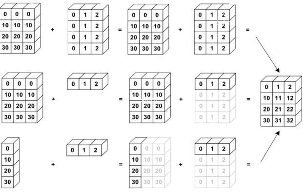
a = np.array([[ 0, 0, 0], [10, 10, 10], [20, 20, 20], [30, 30, 30]]) b = np.array([0, 1, 2]) print(a + b) Out: [[ 0 1 2] [10 11 12] [20 21 22] [30 31 32]]

Center data column-wise a - a.mean(axis=0) Out: array([[-15., -15., -15.], [ -5., -5., -5.], [ 5., 5., 5.], [ 15., 15., 15.]])

(51)

(52)

Scale (center, normalise) data column-wise (a - a.mean(axis=0)) / a.std(axis=0) Out: array([[-1.34164079, -1.34164079, -1.34164079], [-0.4472136 , -0.4472136 , -0.4472136 ], [ 0.4472136 , 0.4472136 , 0.4472136 ], [ 1.34164079, 1.34164079, 1.34164079]]) Examples

Shapes of operands A, B and result: A (2d array): 5 x 4 B (1d array): 1 Result (2d array): 5 x 4 A (2d array): 5 x 4 B (1d array): 4 Result (2d array): 5 x 4 A (3d array): 15 x 3 x 5 B (3d array): 15 x 1 x 5 Result (3d array): 15 x 3 x 5 A (3d array): 15 x 3 x 5 B (2d array): 3 x 5 Result (3d array): 15 x 3 x 5 A (3d array): 15 x 3 x 5 B (2d array): 3 x 1 Result (3d array): 15 x 3 x 5 3.1.9 Exercises Given the array:

X = np.random.randn(4, 2) # random normals in 4x2 array

• For each column find the row index of the minimum value.

• Write a function standardize(X) that return an array whose columns are centered and scaled (by std-dev).

Total running time of the script: ( 0 minutes 0.018 seconds)

(53)

3.2 Pandas: data manipulation

It is often said that 80% of data analysis is spent on the cleaning and small, but important, aspect of data manipulation and cleaning with Pandas.

Sources:

• Kevin Markham: https://github.com/justmarkham

• Pandas doc: http://pandas.pydata.org/pandas-docs/stable/index.html Data structures

• Series is a one-dimensional labeled array capable of holding any data type (inte-gers, strings, floating point numbers, Python objects, etc.). The axis labels are col-lectively referred to as the index. The basic method to create a Series is to call

pd.Series([1,3,5,np.nan,6,8])

• DataFrame is a 2-dimensional labeled data structure with columns of potentially different types. You can think of it like a spreadsheet or SQL table, or a dict of Series objects. It stems from the R data.frame() object.

import pandas as pd import numpy as np

3.2.1 Create DataFrame

columns = ['name', 'age', 'gender', 'job']

user1 = pd.DataFrame([['alice', 19, "F", "student"], ['john', 26, "M", "student"]], columns=columns)

user2 = pd.DataFrame([['eric', 22, "M", "student"], ['paul', 58, "F", "manager"]], columns=columns)

user3 = pd.DataFrame(dict(name=['peter', 'julie'],

age=[33, 44], gender=['M', 'F'], job=['engineer', 'scientist'])) print(user3)

Out:

name age gender job 0 peter 33 M engineer 1 julie 44 F scientist

(54)

3.2.2 Combining DataFrames

Concatenate DataFrame

Concatenate columns (axis = 1).

height = pd.DataFrame(dict(height=[1.65, 1.8])) print(user1, "\n", height)

print(pd.concat([user1, height], axis=1)) Out:

name age gender job 0 alice 19 F student 1 john 26 M student

height 0 1.65 1 1.80

name age gender job height 0 alice 19 F student 1.65

1 john 26 M student 1.80

Concatenate rows (default: axis = 0) users = pd.concat([user1, user2, user3]) print(users)

Out:

name age gender job

0 alice 19 F student 1 john 26 M student 0 eric 22 M student 1 paul 58 F manager 0 peter 33 M engineer 1 julie 44 F scientist Concatenate rows: append user1.append(user2)

Join DataFrame

user4 = pd.DataFrame(dict(name=['alice', 'john', 'eric', 'julie'], height=[165, 180, 175, 171])) print(user4) Out: name height 0 alice 165 1 john 180 2 eric 175 3 julie 171

(55)

Use intersection of keys from both frames merge_inter = pd.merge(users, user4) print(merge_inter)

Out:

name age gender job height

0 alice 19 F student 165

1 john 26 M student 180

2 eric 22 M student 175

3 julie 44 F scientist 171 Use union of keys from both frames

users = pd.merge(users, user4, on="name", how='outer') print(users)

Out:

1 john 26 M student 180.0

2 eric 22 M student 175.0

3 paul 58 F manager NaN

4 peter 33 M engineer NaN

5 julie 44 F scientist 171.0

Reshaping by pivoting

“Unpivots” a DataFrame from wide format to long (stacked) format,

staked = pd.melt(users, id_vars="name", var_name="variable", value_name="value") print(staked)

Out:

name variable value

0 alice age 19 1 john age 26 2 eric age 22 3 paul age 58 4 peter age 33 5 julie age 44 6 alice gender F 7 john gender M 8 eric gender M 9 paul gender F 10 peter gender M 11 julie gender F

12 alice job student 13 john job student 14 eric job student 15 paul job manager

(56)

16 peter job engineer 17 julie job scientist 18 alice height 165

19 john height 180

20 eric height 175

21 paul height NaN

22 peter height NaN 23 julie height 171

“pivots” a DataFrame from long (stacked) format to wide format,

print(staked.pivot(index='name', columns='variable', values='value')) Out:

variable age gender height job name

alice 19 F 165 student

eric 22 M 175 student

john 26 M 180 student

julie 44 F 171 scientist

paul 58 F NaN manager

peter 33 M NaN engineer

3.2.3 Summarizing

users # print the first 30 and last 30 rows

type(users) # DataFrame

users.head() # print the first 5 rows

users.tail() # print the last 5 rows

Descriptive statistics

users.describe(include="all") Meta-information

users.index # "Row names"

users.columns # column names

users.dtypes # data types of each column

users.values # underlying numpy array

users.shape # number of rows and columns

Out: (6, 5)

(57)

3.2.4 Columns selection

users['gender'] # select one column

type(users['gender']) # Series

users.gender # select one column using the DataFrame # select multiple columns

users[['age', 'gender']] # select two columns

my_cols = ['age', 'gender'] # or, create a list...

users[my_cols] # ...and use that list to select columns

type(users[my_cols]) # DataFrame

3.2.5 Rows selection (basic)

iloc is strictly integer position based

df = users.copy()

df.iloc[0] # first row

df.iloc[0, :] # first row

df.iloc[0, 0] # first item of first row

df.iloc[0, 0] = 55

loc supports mixed integer and label based access.

df.loc[0] # first row

df.loc[0, :] # first row

df.loc[0, "age"] # age item of first row

df.loc[0, "age"] = 55 Selection and index

Select females into a new DataFrame df = users[users.gender == "F"] print(df)

Out:

5 julie 44 F scientist 171.0

Get the two first rows using iloc (strictly integer position) df.iloc[[0, 1], :] # Ok, but watch the index: 0, 3

Use loc try:

df.loc[[0, 1], :] # Failed

except KeyError as err: print(err)

(58)

"Passing list-likes to .loc or [] with any missing labels is no longer supported. The␣

˓→following labels were missing: Int64Index([1], dtype='int64'). See https://pandas. ˓→pydata.org/pandas-docs/stable/user_guide/indexing.html#deprecate-loc-reindex-listlike"

Reset index

df = df.reset_index(drop=True) # Watch the index print(df)

print(df.loc[[0, 1], :]) Out:

2 julie 44 F scientist 171.0 name age gender job height 0 alice 19 F student 165.0

3.2.6 Sorting

3.2.7 Rows iteration df = users[:2].copy()

iterrows(): slow, get series,read-only • Returns (index, Series) pairs.

• Slow because iterrows boxes the data into a Series. • Retrieve fields with column name

• Don’t modify something you are iterating over. Depending on the data types, the iterator returns a copy and not a view, and writing to it will have no effect.

for idx, row in df.iterrows(): print(row["name"], row["age"]) Out:

alice 19 john 26

itertuples(): fast, get namedtuples,read-only

• Returns namedtuples of the values and which is generally faster than iterrows. • Fast, because itertuples does not box the data into a Series.

• Retrieve fields with integer index starting from 0.

• Names will be renamed to positional names if they are invalid Python identifier

(59)

for tup in df.itertuples(): print(tup[1], tup[2]) Out:

alice 19 john 26

iter using loc[i, . . . ]: read andwrite for i in range(df.shape[0]):

df.loc[i, "age"] *= 10 # df is modified

3.2.8 Rows selection (ﬁltering)