To be or not to be quadratic (with X-Fem)

HAL Id: hal-01923676

https://hal.archives-ouvertes.fr/hal-01923676

HAL is a multi-disciplinary open access archive for the deposit and dissemination of sci-entific research documents, whether they are pub-lished or not. The documents may come from teaching and research institutions in France or abroad, or from public or private research centers.

L’archive ouverte pluridisciplinaire HAL, est destinée au dépôt et à la diffusion de documents scientifiques de niveau recherche, publiés ou non, émanant des établissements d’enseignement et de recherche français ou étrangers, des laboratoires publics ou privés.

To be or not to be quadratic (with X-Fem)

Nunziante Valoroso, Alexandre Martin

To cite this version:

Nunziante Valoroso, Alexandre Martin. To be or not to be quadratic (with X-Fem). 13e colloque national en calcul des structures, Université Paris-Saclay, May 2017, Giens, Var, France. �hal-01923676�

CSMA 2017

To be or not to be quadratic (with X-Fem)

Nunziante Valoroso1, Alexandre Martin2

1_{Dipartimento di Ingegneria, Università di Napoli Parthenope, nunziante.valoroso@uniparthenope.it} 2_{IMSIA, UMR EDF CEA CNRS ENSTA ParisTech, Université Paris Saclay, alexandre.martin@cnrs.fr}

Abstract — A novel implementation of the eXtended Finite Element Method that makes use of qua-dratic elements is discussed. The present formulation is shown to behave fairly better compared to usual quadratic elements enriched with Heaviside functions in that both the number of unknowns and the condition number of element matrices considerably decrease with respect to a classical second order scheme. A representative example demonstrates the capabilities of the proposed approach.

Keywords — Fracture, X-Fem, quadratic elements.

1

Introduction

There is no question that the quality of eXtended Finite Element (X-Fem) solutions to problems with discontinuities has dramatically improved in the last decade, nor can it be doubted that there is still a long way to go.

For instance, most X-Fem implementations rely upon use of either linear triangles/quadrilaterals in 2D or linear tetrahedra/hexahedra in 3D. Aiming to get better performances and higher order convergence properties the X-Fem approximation could be modified to be quadratic. However, despite all expected beneficial effects of quadratic elements, in published X-Fem literature almost all but a few authors, see e.g [1, 2, 3, 4], choose not to be quadratic. The main motivation beyond this choice is that in the present context a successful implementation of higher order elements is conditional to the possibility that element matrices created by X-Fem are not ill-conditioned, that in a sense is intrinsic to the method itself.

2

X-Fem for discontinuities

Generally speaking, the X-Fem concept can be regarded as a special case of the partition of unity paradigm [5], the basic underlying idea being the augmentation of the approximation space generated by standard finite element shape functions. This is obtained in turn via suitable enrichment functions that incorporate some a priori knowledge about the solution of the problem under consideration. For instance, in fracture mechanics displacement discontinuities can be introduced via the generalized Heaviside func-tion :

H(x) = h(ϕ(x)) = (

+1 if ϕ(x) ≥ 0

−1 if ϕ(x) < 0 (1)

whereϕ(x) is a function that defines the interface position, e.g. typically a signed distance function. At

any point x of the finite element mesh the displacement approximation is then obtained as : uh(x) = numnp

∑

∑

where φi(x) and ψj(x) are standard finite element shape functions and numnp is the number of nodal

points. The degrees of freedom of the regular part of the interpolated displacement field are denoted by ai, whereas the additional degrees of freedom associated with the Heaviside enrichment are denoted as

qj. The latter are active on the set of nodes NH whose support is bisected by the interface ; therefore, at

the element level the matrices do not have in general equal dimensions.

In usual X-Fem implementations the functions ψj that are used to describe the jumps are taken

strictly required by the method since for the Heaviside function to be exactly represented it is sufficient that functionsψj do comply with the partition of unity property. Likewise, the degrees of freedom qj of

the jumps are usually attached to the same nodal points carrying the unknowns ai of the regular part of

the displacement. Once again, this is not a compulsory condition but only a customary choice, probably originating from the fact that, at least for fracture mechanics problems, most X-Fem implementations make use of linear elements.

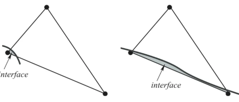
Unlike continuous elements, increasing the order of the standard shape functions in the X-Fem ap-proximation (2) is not sufficient to guarantee an improvement in performances and convergence proper-ties. Actually, when considering the Heaviside enrichment, severe ill-conditioning is likely to occur for elements crossed by an interface whenever the area or volume ratio between the two parts on the opposite sides of the interface is very small, see e.g. Figure 3. In such cases one of the Heaviside-enriched func-tions describing the displacement jumps tend to coincide with one standard continuous shape function, whereby the stiffness matrix becomes rank-deficient.

interface interface

Figure 1 – interface positions that cause ill-conditioning.

In practical applications there is no way to avoid the occurrence of discontinuities arbitrarily close to nodes or element sides within the mesh, since by its very definition an X-Fem interface can be arbi-trarily positioned within a mesh. Special treatments of this pathological situation have been presented in [2, 3, 6], that make use either of a pre-conditioner to eliminate linear dependencies between standard shape functions and enrichment functions or rely upon geometric or stiffness weighting criteria to decide whether to enrich a given node. Unfortunately, the above treatments seems to be not robust enough to let quadratic lagrangian elements perform well [4].

In view of general industrial applications, where simplicity of model preparation and mesh generation are essential requirements as much as good accuracy and convergence properties, to be quadratic with X-Fem we design elements including corner rotations as degrees of freedom. Such rotations are usually termed drilling degrees of freedom in reference to their tendency to twist nodes about the normal to the element surface.

3

Quadratic elements with drilling rotations

Finite element methods designed to include corner rotations have been discussed in many papers since the 1980s. Earlier works did not succeed in the derivation of elements with an independent rotation field in the sense of Reissner [7] either due to the presence of zero-energy modes or to the instability of finite dimensional formulations despite the well-posedness of the continuum problem.

A consistent variational framework for problems including rotational degrees of freedom has been presented by Hughes and Brezzi in [8], where a methodology is provided to obtain a robust finite element method that permits the representation of drilling rotations using a C(0)interpolation.

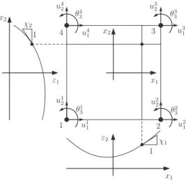
In the following it is summarized the derivation of the quadratic quadrilateral sketched in Figure 2 ; key points in setting the functional from which the element matrices are obtained are as follows :

1. the stress tensor is not a priori assumed to be symmetric ;

2. the drilling rotation is identified with the component of the infinitesimal continuum rotation normal to the plane of the element ;

These conditions are both enforced in weak form using the following functional, see [8] pag 115 : Πγ(u,θ,Tu) =1 2 Z ΩE (∇u) s_·(∇u)s_dΩ+Z Ω((∇u) u_{− θ) · T}u_dΩ−γ −1 2 Z ΩT u_·Tu_dΩ−Z Ωf · u dΩ (3)

whereE is the 2D plane elasticity matrix, f are the body forces, u is the displacement field, θ and T are the

infinitesimal rotation and stress, and the symbols(·)s_and(·)u_{stand for symmetric and skew-symmetric}

part of the argument, respectively. Moreover, the constantγin (3) is a positive penalty parameter that in linear elastostatics ensures that the discrete variational problem inherits the ellipticity property from its continuum counterpart. x1 x1 x2 x2 ε1 ε2 _χ1 χ2 u1 1 u 2 1 u3 1 u4 1 u1 2 u22 u3 2 u4 2 θ1 3 θ23 θ3 3 θ4 3 1 1 1 2 3 4

Figure 2 – quadrilateral element with drilling degrees of freedom.

The normal rotation field over the quadrilateral is interpolated by the standard bilinear shape func-tions whereas the in-plane displacement components are approximated using an Allman-like interpola-tion. In matrix notation one has :

u= " u1 u2 # = 4

∑

∑

∑

1,uI2,θI3]T being the displacement vector at node I and a the vector collecting all the element

displacement components. The discretized counterpart of the functional (3) that is arrived at reads :

Πh γ(a,τ) = 1₂ Z ΩE Ba · Ba dΩ+ Z ΩbaτdΩ− 1 2γ −1Z Ωτ 2_dΩ−Z Ωf · Na dΩ (7)

where the parameterτrepresents the interpolation for the skew-symmetric stress ; since no continuity is needed for it, an element-wise constant interpolation is chosen and the unknownτis condensed out at the element level. Therefore, the element stiffness matrix is obtained by adding to the usual stiffness matrix

the rank-one correction : _γ

meas(Ω) Z

Ω(b ⊗ b) dΩ (8)

4

Numerical example

To demonstrate the current element capabilities a simple problem is considered that consists of a single element, either a standard serendipity element (Q8) or a quadrilateral with drilling rotations (QD4), occupying the domain[−1, 1] × [−1, 1]. The element is cut by an X-Fem interface parallel to one of its

sides and the discontinuity is described via the Heaviside function (1).

The position of the interface on the element is parametrized through the abscissaε(ε= 0 corresponds

to the left side of the element). No boundary condition is imposed on the element, that it is completely free ; therefore it possesses six rigid-body motions, i.e. the three rigid body motions of the underlying continuum element plus three extra rigid-body motions due to the presence of the X-Fem interface.

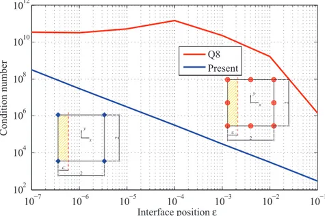
In figure 3 is depicted the condition number of the Q8 and QD4 element stiffness matrices at varying interface position. The superior performance of the QD4 element, that remains workable for up to ε=

1 · 10−7, is immediately recognized whereas the stiffness matrix of the Q8 element is already almost singular forε= 1 · 10−3_. 10−7 10−6 10−5 10−4 10−3 10−2 10−1 102 104 106 108 1010 1012 Condi ti on num b er Interface position ε Q8 Present

Figure 3 – conditioning of element matrices.

References

[1] K.W. Cheng and T.P. Fries. Higher-order xfem for curved strong and weak discontinuities. International Journal for Numerical Methods in Engineering, 82(5) :564–590, 2010.

[2] E. Béchet, H. Minnebo, N. Moës, and B. Burgardt. Improved implementation and robustness study of the x-fem for stress analysis around cracks. International Journal for Numerical Methods in Engineering, 64(8) :1033– 1056, 2005.

[3] K. Dreau, N. Chevaugeon, and N. Moës. Studied x-fem enrichment to handle material interfaces with higher order finite element. Computer Methods in Applied Mechanics and Engineering, 199(29-32) :1922 – 1936, 2010.

[4] M. Ndeffo, P. Massin, N. Moës, A. Martin, and S. Gopalakrishnan. On the construction of approximation space to model discontinuities and cracks with linear and quadratic elements. 2016. submitted for publication. [5] J.M. Melenk and I. Babuska. The partition of unity finite element method : Basic theory and applications.

Computer Methods in Applied Mechanics and Engineering, 139(1) :289 – 314, 1996.

[6] M. Siavelis, M. L. E. Guiton, P. Massin, and N. Moës. Large sliding contact along branched discontinuities with x-fem. Computational Mechanics, 52(1) :201–219, 2013.

[7] E. Reissner. A note on variational principles in elasticity. International Journal of Solids and Structures, 1 :93–95, 1965.

[8] T.J.R. Hughes and F. Brezzi. On drilling degrees of freedom. Computer Methods in Applied Mechanics and Engineering, 72(1) :105–121, 1989.