Video-based analysis of Gait pathologies

Université de Montréal

Video-based Analysis of Gait Pathologies

par

Hoang Anh Nguyen

Département d’informatique et de recherche opérationnelle Faculté des arts et des sciences

Thèse présentée à la Faculté des études supérieures en vue de l’obtention du grade de Philosophiæ Doctor (Ph.D.)

en informatique

Decembre, 2014

c

RÉSUMÉ

L’analyse de la marche a émergé comme l’un des domaines médicaux le plus im-portants récemment. Les systèmes à base de marqueurs sont les méthodes les plus fa-vorisées par l’évaluation du mouvement humain et l’analyse de la marche, cependant, ces systèmes nécessitent des équipements et de l’expertise spécifiques et sont lourds, coûteux et difficiles à utiliser. De nombreuses approches récentes basées sur la vision par ordinateur ont été développées pour réduire le coût des systèmes de capture de mou-vement tout en assurant un résultat de haute précision. Dans cette thèse, nous présentons notre nouveau système d’analyse de la démarche à faible coût, qui est composé de deux caméras vidéo monoculaire placées sur le côté gauche et droit d’un tapis roulant. Chaque modèle 2D de la moitié du squelette humain est reconstruit à partir de chaque vue sur la base de la segmentation dynamique de la couleur, l’analyse de la marche est alors effectuée sur ces deux modèles. La validation avec l’état de l’art basée sur la vision du système de capture de mouvement (en utilisant le Microsoft Kinect) et la réalité du ter-rain (avec des marqueurs) a été faite pour démontrer la robustesse et l’efficacité de notre système. L’erreur moyenne de l’estimation du modèle de squelette humain par rapport à la réalité du terrain entre notre méthode vs Kinect est très prometteur: les joints des angles de cuisses (6,29◦contre 9,68◦), jambes (7,68◦contre 11,47◦), pieds (6,14◦contre 13,63◦), la longueur de la foulée (6.14cm rapport de 13.63cm) sont meilleurs et plus stables que ceux de la Kinect, alors que le système peut maintenir une précision assez proche de la Kinect pour les bras (7,29◦ contre 6,12◦), les bras inférieurs (8,33◦ contre 8,04◦), et le torse (8,69◦contre 6,47◦). Basé sur le modèle de squelette obtenu par chaque méthode, nous avons réalisé une étude de symétrie sur différentes articulations (coude, genou et cheville) en utilisant chaque méthode sur trois sujets différents pour voir quelle méthode permet de distinguer plus efficacement la caractéristique symétrie / asymétrie de la marche. Dans notre test, notre système a un angle de genou au maximum de 8,97◦ et 13,86◦ pour des promenades normale et asymétrique respectivement, tandis que la Kinect a donné 10,58◦et 11,94◦. Par rapport à la réalité de terrain, 7,64◦et 14,34◦, notre système a montré une plus grande précision et pouvoir discriminant entre les deux cas.

ABSTRACT

Gait analysis has emerged as one of the most important medical field recently due to its wide range of applications. Marker-based systems are the most favoured methods of human motion assessment and gait analysis, however, these systems require specific equipment and expertise, and are cumbersome, costly and difficult to use. Many re-cent computer-vision-based approaches have been developed to reduce the cost of the expensive motion capture systems while ensuring high accuracy result. In this thesis, we introduce our new low-cost gait analysis system that is composed of two low-cost monocular cameras (camcorders) placed on the left and right sides of a treadmill. Each 2D left or right human skeleton model is reconstructed from each view based on dy-namic color segmentation, the gait analysis is then performed on these two models. The validation with one state-of-the-art vision-based motion capture system (using the Mi-crosoft Kinect v.1) and one ground-truth (with markers) was done to demonstrate the robustness and efficiency of our system. The average error in human skeleton model estimation compared to ground-truth between our method vs. Kinect are very promis-ing: the joints angles of upper legs (6.29◦vs. 9.68◦), lower legs (7.68◦ vs. 11.47◦), feet (6.14◦ vs. 13.63◦), stride lengths (6.14cm vs. 13.63cm) were better and more stable than those from the Kinect, while the system could maintain a reasonably close accu-racy to the Kinect for upper arms (7.29◦ vs. 6.12◦), lower arms (8.33◦ vs. 8.04◦), and torso (8.69◦vs. 6.47◦). Based on the skeleton model obtained by each method, we per-formed a symmetry study on various joints (elbow, knee and ankle) using each method on two different subjects to see which method can distinguish more efficiently the sym-metry/asymmetry characteristic of gaits. In our test, our system reported a maximum knee angle of 8.97◦and 13.86◦for normal and asymmetric walks respectively, while the Kinect gave 10.58◦ and 11.94◦. Compared to the ground-truth, 7.64◦ and 14.34◦, our system showed more accuracy and discriminative power between the two cases.

CONTENTS

RÉSUMÉ . . . iii

ABSTRACT . . . iv

LIST OF TABLES . . . viii

LIST OF FIGURES . . . x

LIST OF ABBREVIATIONS . . . xviii

NOTATION . . . xix

CHAPTER 1: INTRODUCTION . . . 1

CHAPTER 2: LITERATURE REVIEW . . . 3

2.1 Model free . . . 6

2.1.1 Probabilistic assemblies of parts . . . 6

2.1.2 Example-based methods . . . 7

2.2 Direct model use . . . 11

2.2.1 3D pose estimation from multiple views . . . 12

2.2.2 2D/3D pose estimation from monocular view . . . 13

2.2.3 Learnt motion models . . . 16

2.2.4 3D pose estimation from depth sensor . . . 16

CHAPTER 3: METHODOLOGY . . . 18

3.1 System overview . . . 18

3.2 Preprocessing . . . 20

3.3 Pose estimation . . . 26

3.3.1 Head and torso . . . 26

3.3.3 Upper arm . . . 35

3.3.4 Leg reconstruction . . . 38

3.3.5 3D foot estimation and automatic gait cycle segmentation . . . 39

3.4 Synchronization between two cameras . . . 43

CHAPTER 4: EXPERIMENTATION AND VALIDATION . . . 47

4.1 Synchronization between cameras . . . 47

4.2 Validation with the Kinect and ground-truth measurements . . . 49

CHAPTER 5: APPLICATION TO GAIT ASYMMETRY ASSESSMENT 65 5.1 Methodology . . . 65

5.1.1 Overview . . . 65

5.1.2 Asymmetry measurements . . . 68

5.2 Experimentation . . . 69

5.3 Discussion . . . 71

CHAPTER 6: CONCLUSION AND FUTURE WORK . . . 76

BIBLIOGRAPHY . . . 78 APPENDIX A: . . . 86 A.1 Context . . . 86 A.2 Abstract . . . 86 A.3 Introduction . . . 87 A.4 Overview . . . 88

A.5 Full perspective technique . . . 88

A.6 Skeleton reconstruction algorithm . . . 90

A.6.1 Estimating foot, knee and pelvic points . . . 91

A.6.2 Estimating torso and head . . . 92

A.6.3 Estimating shoulders, elbows and hands . . . 92

APPENDIX B: . . . 95

B.1 Context . . . 95

B.2 Methodology . . . 95

B.2.1 3D shoulder . . . 96

B.2.2 3D elbow and hand . . . 100

LIST OF TABLES

4.I Synchronization error ε (in number of frames) between our left, right camcorders and the Kinect. . . 49 4.II Average of absolute differences of each human segment (see Fig. 3.2)

from our method (columns 1 and 3) and from the Kinect SDK (columns 2 and 4) compared to the ground-truth skeleton model of subject 1 in two tests. The average stride length error (in both ab-solute value in centimetre and in percent compared to mean stride length) are also shown. These results were calculated over 20 cy-cles. The values in bold indicate which method (our method or Kinect) produced the largest error. . . 63 4.III Average of absolute differences at three joints of interest (knee,

elbow and ankle, see Fig. 3.2 blue arrows) from our method (columns 1 and 3) and from the Kinect SDK (columns 2 and 4) compared to the ground-truth skeleton model of subject 1 in two tests. These results were calculated over 20 cycles. The values in bold indicate which method (our method or Kinect) produced the largest error. . 63 5.I Asymmetry measures (degrees) compared with the markers

(ground-truth) by the camcorders and the Kinect on subject 1. These results were calculated over 10 cycles. (A) Normal walk. (B) Left asym-metry walk. (C) Right asymasym-metry walk. . . 75 5.II Asymmetry measures (degrees) compared with the markers

(ground-truth) by the camcorders and the Kinect on subject 2. These results were calculated over 10 cycles. (A) Normal walk. (B) Left asym-metry walk. (C) Right asymasym-metry walk. . . 75

5.III The average of absolute difference (centimetre) between left and right stride length calculated by the markers (ground-truth), the camcorders and the Kinect on subjects 1 and subject 2. These results were calculated over 10 cycles. (A) Normal walk. (B) Left asymmetry walk. (C) Right asymmetry walk. . . 75 A.I Two different sets of relative lengths of segments used in the

com-putation of human model. MC = Motion Capture. L = Literature. The coefficient i has been added in the last column to consider variation of the human size. . . 89

LIST OF FIGURES

1.1 (A) Our system consists of one treadmill and two camcorders on the left and right side of the treadmill. Four light sources were placed at the four corners of the room to assure good light diffu-sion. (B) Our system in real life. . . 2 2.1 A detailed gait cycle description [65]. . . 3 2.2 Anatomical planes in a human [66]. . . 4 2.3 The Vicon system makes uses of infrared reflective markers on the

subject body parts [67]. . . 5 2.4 The tree structured representation of human body parts used in [9]. 7 2.5 The feature histogram of orientated gradient (HOG) is widely used

in the human detection area [12]. . . 8 2.6 The fundamental steps of the skeletal detection technique was

in-troduced in [21]. . . 10 2.7 Result shows the superior performance of ISA against other

tech-niques [24]. . . 13 2.8 The first row shows the result of LLM and the second row shows

the result of FJM. (i) to (iv) show results obtained at iteration 1, 3, 5, 10 respectively. (v) shows the final 3D pose. The convergence speed of FJM is clearly superior than LLM (source [25]). . . 14 2.9 The 3D poses disambiguation from uncertainty 2D poses is

intro-duced in [30]. . . 15 2.10 (A) In [1], the gait is obtained by first finding body contours (left

image), then performing ellipse estimation for each body part within these contours. (B). The xyt block is used to distinguish left leg from right leg. . . 16

3.1 Overview of our system: each processing of each camera is treated independently to get its corresponding skeleton model. This ar-chitecture encourages parallel computing to speed up the system performance. . . 19 3.2 The left and right human skeleton models are used in our system.

Each model consists of 9 nodes and 8 joints allowing more com-plicated gait analysis. Red lines connect body joints together. Blue arrows represent our 3 joint angles of interest at elbow, knee and ankle. . . 20 3.3 (A) The square block: the output of points A and B are

deter-mined by Q4 and Q2 respectively. The straight line edge is not

preserved.(B) The circular block is divided into 8 sectors in [27]. The sectors (with thick-line) determine the final output. . . 21 3.4 (A) The original image. (B) Output of Kuwahara filter with visible

blocking effects. (C) Output of [27]. . . 22 3.5 Work-flow of our system which briefly introduces each step . . . 24 3.6 The ellipse fitting result from [69] (solid line) compared to other

approaches. (Source [69]). . . 28 3.7 Torso estimation comparison between [51] (blue line), ours (green

line) and ground-truth (red line). Our method is very close to the ground-truth in all three cases, especially better than [51] in (A) where the subject’s body shape does not have ellipse-form, and (C) where the clothes distort the body shape. . . 31

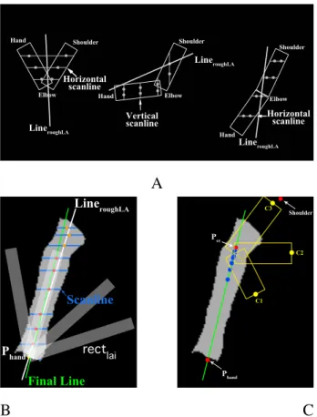
3.8 (A) Scanline type decision (horizontal or vertical) depends on Line_roughLA orientation and hand location. (B) Lower arm estimation using lin-ear least squares on scanline clustering. The white line represents the rough line Line_roughLA, red dots are scanline centres that be-long to the lower arm, while the orange dots do not. The final green line is estimated by performing linear least squares on the red dot set. (C) Sampling technique for estimating the upper arm: blue points follow a Gaussian distribution whose centre is located at the known elbow. Many yellow rectangles, such as C1,C2,C3

representing three candidates of upper arm, were generated. . . . 33 3.9 A chessboard is placed on the treadmill to compute the

homog-raphy H between chessboard plane and image plane. The world origin is locate at O; red, cyan and blue arrows represent the X ,Y and Z axis respectively. All green lines, which are parallel to each other in real world, now intersect at one vanishing point in image plane. . . 40 3.10 The overview of our 3D foot trajectory estimation. (A) 2D foot

locations (green line) in one gait cycle in image space. (B) 3D tra-jectory (red line) retrieved in world space in which Pmin, Pmax

rep-resent the minimum point and maximum point respectively along the horizontal axis. . . 43 3.11 The synchronization process between two cameras . . . 45 4.1 Our synchronization result for 3 cameras: left camcorder (red line),

right camcorder (blue line) and Kinect (magenta line). (A) Before doing synchronization. (B) After doing synchronization with the left camera as the reference. . . 48

4.2 Graphs representing the relation between N_switch and error ε for the right camera (red line) and for Kinect (blue line). The error significantly dropped until Nswitch= 3, and less significantly after

that. . . 49 4.3 Variation of foreshortening level ρua of upper arm (red line) and

foreshortening level ρla of forearm (blue line) for subject 1 (A)

and subject 2 (B). . . 51 4.4 Our skeleton reconstruction on subject 1. The first row shows

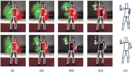
some of our testing frames captured from the left camera, the sec-ond row shows their correspsec-onding frames from the right camera. Red lines indicate the ground-truth formed by red markers placed on the subject’s body, our pose estimation produced the green lines and green ellipses. The third row shows the 3D skeleton from the Kinect SDK. The Kinect tends to fail in cases C,D where it could not see the lower leg due to occlusions. . . 53 4.5 Our skeleton reconstruction on subject 2. Just like subject 1, the

Kinect failed in cases C,D where it could not see the lower leg due to occlusions. . . 54 4.6 Ten typical curves which correspond to 10 consecutive cycles

pro-duced by our method. Each gait cycle duration varies very lightly from 38 to 41 frames. For convenience, we simply cut all cycles at frame 38 when calculating the average curve over 20 cycles. . . 55

4.7 Average curve representing the angle variation at the left knee es-timated from ground-truth (blue line), Kinect SDK (red line) and our method (green line) within a gait cycle. The horizontal axis is the frame number in a walking cycle. The first row is the result observed from Test 1, the second row is from Test 2. Our method outperformed the Kinect SDK in Test 2 and successfully located the minimum knee joint angle while the Kinect SDK failed due to lower leg occlusions. The curves were obtained by averaging 20 cycles. . . 56 4.8 Average curves representing the angle variation at the left elbow

estimated from ground-truth (blue line), Kinect SDK (red line) and our method (green line) within a gait cycle. The curves were ob-tained by averaging 20 cycles. The results from the three methods were quite similar in this case. . . 57 4.9 Average curves representing the angle variation at the left ankle

es-timated from ground-truth (blue line), Kinect SDK (red line) and our method (green line) within a gait cycle. The curves were ob-tained by averaging 20 cycles. The ankle angle estimated by the Kinect is inconsistent and produces much larger bias errors than ours. . . 58 4.10 (A) The left camera forms an angle of 80◦ to the walking

direc-tion (wrong). (B) The left camera forms an angle of 90◦ to the walking direction (correct). The effects of (A) to the final skeleton estimation were empirically negligible. . . 60

4.11 The upper (blue dash line) and lower boundaries (red dash lines) calculated at knee around the average curve for subject 1. The up-per curve is obtained by adding the standard deviation to the aver-age curve. The lower curve is obtained by subtracting the standard deviation to the average curve. The standard deviations were cal-culated over 20 cycles. (A) Results from our method. (B) Results from the Kinect. . . 61 4.12 The upper (blue dash line) and lower boundaries (red dash lines)

calculated at elbow around the average curve for subject 1. The upper curve is obtained by adding the standard deviation to the av-erage curve. The lower curve is obtained by subtracting the stan-dard deviation to the average curve. The stanstan-dard deviations were calculated over 20 cycles. (A) Results from our method. (B) Re-sults from the Kinect. . . 62 4.13 The upper (blue dash line) and lower boundaries (red dash lines)

calculated at ankle around the average curve for subject 1. The up-per curve is obtained by adding the standard deviation to the aver-age curve. The lower curve is obtained by subtracting the standard deviation to the average curve. The standard deviations were cal-culated over 20 cycles. (A) Results from our method. (B) Results from the Kinect. . . 62 5.1 The authors in [53] summarized popular equations to quantify gait

symmetry. (Source: [53]) . . . 66 5.2 Our system consists of one treadmill and two cameras on the left

and right sides of the treadmill. Four light sources are placed at the four corners of the room to ensure good light diffusion. . . 67

5.3 The first row shows some of our testing frames captured from the left camera, the second row shows their corresponding frames from the right camera. Red lines indicate the ground-truth formed by red markers placed on the subject’s body, our pose estimation produced the green lines and green ellipses. The third row shows the 3D skeleton from the Kinect SDK. . . 68 5.4 From top to bottom, we shift the right knee angle curve (dash blue

curve) while the left knee (red curve) remains stationary by in-creasing ∆. The bottom graph gives the lowest error δ used as asymmetry measure. . . 70 5.5 Angle changes at knee. Solid and dash red lines represent the

an-gle changes at the left knee joint for normal and abnormal cases respectively within T_id seconds. Solid and dash blue lines repre-sent the angle changes at the right knee joint for normal and abnor-mal cases respectively within Tid seconds. In the case of abnormal

walk, the dash lines demonstrate clearly the broken symmetry be-tween left and right parts. . . 72 5.6 Angle changes at elbow, same color configuration as Fig 5.5. . . . 73 5.7 Angle changes at ankle, same color configuration as Fig 5.5. . . . 74 A.1 The 3D model used to estimate the arm. Plane p, represented by

the red triangle, is created with 3 points: neck, left and right hips. S, E, H indicate the left shoulder, left elbow, left hand respectfully. 91 A.2 The results obtained by applying the reconstruction algorithm to

calibrated images. Left column contains the original images with different poses. The middle and the last columns show the estima-tion results with different view direcestima-tions. . . 94 B.1 The projection of shoulder (blue circle) onto the ground (green

circle) should lie inside the foot range which is indicated by the 2-head arrow. . . 97

B.2 3D shoulder assessment overview: particles (red points) are gener-ated around P_shoulderinit which is deduced from Pv f oot. The first layer

keeps only blue points which represent a ray from camera. The second layer evaluates each remaining candidate siand its two

cor-responding elbow candidates (e1and e2) by finding the one having

the angle to sagittal plane (α1and α2) closest to the ρua constraint

(Equation B.1). . . 98 B.3 (A) Elbow and hand candidates generated by weak perspective

technique in [48]. Each path from shoulder to hand represents an arm pose, there are four paths in total (c1, c2, c3, c4). (B) Dynamic

programming: each cell of the table is deduced by taking infor-mation from all cells in the previous column. The shortest path is found by locating the minimum cell in the last column, then tracing backward to the first column. . . 101 B.4 Arm 3D reconstruction under light foreshortening problem. First

column is our 2D arm detection (green lines and elbow is marked as green circle), the second and third columns show our results (blue lines) and Kinect’s (red lines) from left and right view side in 3D space respectively. In these cases, as we can see, the elbow angle from our results are closed to that from Kinect. . . 104 B.5 Arm 3D reconstruction in heavy foreshortening problem. In these

cases, the errors are clearer in the first and second row, in which the lower arm joint length is not very accurate. The last row, in which the elbow is badly estimated, produces the 3D arm reconstruction failure. . . 105

LIST OF ABBREVIATIONS

APF Annealed particle filter DS Deformable structure EM Expectation maximization FJM Fixed joint model

GAIMS Gait measuring system

HOG Histogram of oriented gradient ICP Iterative closest point

IR Infrared

ISA Interacting simulated annealing LED Light-emitting diode

LLM Loose limb model

MCMC Markov chain Monte Carlo MOCAP Motion capture

PF Particle filter

PFICP Particle filter + Iterative closest point PS Pictorial structure

RGB-D Red-Green-Blue + Depth RF Random forest

RRF Random regression forest SDK Software development kit SVM Support vector machine

NOTATION

Ns Predefined number of sectors

s_i Sector i

w_i Weighting function for sector i

k Number of clusters in k-means algorithm (µskin, σskin) mean and variance of the skin model

BB₁ Bounding box of the whole silhouette

BB2 Bounding box of the half lower part of the silhouette

< L_c, R_c> Left and right contours of the torso model N_c The total number of points of both Lcand Rc

{x_li, y_li}N x-component and y-component of point li in Lc

{x_ri, y_ri}_N x-component and y-component of point ri in Rc

k Frame number k

N_skinli Number of frames where an contour point x_li, y_liis skin N_skinri Number of frames where an contour point xri, yriis skin

P_{f orehead} The 2D forehead joint location of our 2.5D skeleton model P_chin The 2D chin joint location of our 2.5D skeleton model P_shoulder The 2D shoulder joint location of our 2.5D skeleton model

P_hip The 2D hip joint location of our 2.5D skeleton model P_hand The 2D hand joint location of our 2.5D skeleton model P_elbow The 2D elbow joint location of our 2.5D skeleton model

P_ankle The 2D ankle joint location of our 2.5D skeleton model

Pce The furthest possible elbow joint position along the forearm orientation

P_O The origin coordinate of the 3D world space

cli The closest edge point to the i-th point of the new left contour Lp that

has the same y-value

cri The closest edge point to the i-th point of the new right contour Rpthat

has the same y-value

Et The cost function used to evaluate the new torso shape < Lp, Rp>

Map_skin A binary image in which the value of skin pixels is 1, and the rest is 0 L_LA Forearm segment length

LUA Upper arm segment length

rectlai A fixed size rectangle used to capture forearm orientation. w_lar Width of rectlai

List_rectla List of rectangle rectlai generated with respect to the hand joint location P_hand

Line_LA The 2D line represents the forearm orientation S_elbow List of elbow candidates

Si_elbow The i-the candidate of Selbow

S_shoulder List of shoulder candidates S_shoulderj The j-the candidate of S_shoulder

S_candidates List of combined candidates for constructing 2D arm ρua Foreshortening level of upper arm

ρla Foreshortening level of forearm

E_UAi Cost function to evaluate an arm candidate i of Scandidates

H i

ua1 First term of EUAi

H i

ua2 Second term of EUAi

αuarm Constant to control the importance ofHua1i toHua2i

N_f Frame number of 3D foot trajectory H Homography matrix

θf The 3D line represent the walking orientation of a foot

P_min The top left point of the 3D foot trajectory when foot is on the ground Pmax The top right point of the 3D foot trajectory when foot is on the ground

L_{tra ject} The line that connects Pminand Pmax

L2d_{tra ject} The projection of Ltra ject into image space

Lm_stride The stride length of a sub-map m L_stride The final average stride length

T_i Time that we turn off the light (i = 0, 2, 4, etc.) Tj Time that we turn on the light (i = 1, 3, 5, etc.)

N_switch Number of turn off-turn on the light ∆ Time delay

c Camera r Reference

ε The minimized mean error of multiple cameras synchronization with respect to ∆

T_id Constant waiting time between two consecutive asymmetry calculation steps

Ra A curve measured at one of the right joints (knee, elbow, ankle, etc.)

L_a A curve measured at one of the left joints (knee, elbow, ankle, etc.) δ Asymmetry index

Fρua Mapping function that maps one value of ρua into degrees.

p_{v f oot} The 2D projection of Pshoulder into L2dtra ject

P_{v f oot} The corresponding 3D point of pv f oot

H_shoulder The distance from shoulder to the ground according to [50] P_shoulderinit The initial position of 3D shoulder deduced from Pv f oot

pt_s A particle which is an candidate of 3D shoulder pte A particle which is an candidate of 3D elbow

E_S Cost function to evaluate an shoulder candidate N_p Number of particles

N_l Number of frames that are used to reconstruct the 3D arm

DP A (4 × Nl) table used in finding the most consistent movement of arm

E_eh Cost function value of a cell in DP

P_shoulder3d The 3D shoulder joint location of our 3D arm model P_elbow3d The 3D elbow joint location of our 3D arm model

(Xw,Yw, Zw) The x,y,z coordinates of a 3D point in world space (Xc,Yc, Zc) The x,y,z coordinates of a 3D point in camera space

(x, y) The x,y coordinates of a 2D point in image space f Focal length

(px, py) Horizontal and vertical effective pixel size

CHAPTER 1

INTRODUCTION

Nowadays, in order to diagnose abnormal gait patterns in medical clinics, gait anal-ysis systems play a crucial role. Among state-of-the-art systems, motion capture (MO-CAP) is without a doubt the most popular one due to its very high precision. Each pa-tient is asked to wear several infrared (IR) reflective markers so that multiple IR cameras can observe the signal. Such systems cost thousands of dollards and require complex knowledge from the operator to make it function properly. In recent years, along with the development of computer hardware, video-based human motion capture and analy-sis has achieved huge advances. Along with the appearance of RGB-D cameras on the market, high-accuracy motion capture can be archived in real time based on this new technology. Most of these systems aim for recognizing human gesture only (based on the upper body), so their application in gait analysis, which mostly focuses on lower body, has not been fully studied and tested yet. In this thesis, we focus on developing a new low-cost video-based gait analysis system that can automatically reconstruct a 2.5D human skeleton over time and then analyze the gait to detect related pathological problems. Combining multiple vision and optimization techniques to create such a sys-tem that can outperform vision-based state-of-the-art syssys-tem in gait analysis, that is the principal contribution of this thesis.

We introduce such a system that is composed of a treadmill associated with two low-cost color camcorders (see Fig 1.1). Our system automatically reconstructs the human skeleton model (see Fig 3.2) of the patient walking on the treadmill from a recorded video sequence. Gait asymmetry problems and other gait disorders are then detected by observing the angle variations between various joints of the skeleton through time. Our ultimate purpose when designing this system is to obtain higher accuracy of skeleton re-construction than the current low-cost state-of-the-art (Kinect) for efficient gait analysis by adding some necessary but easy-to-realize constraints to the estimating process. The processing on each camera is designed to work independently to ease the system setup in

A B

Figure 1.1: (A) Our system consists of one treadmill and two camcorders on the left and right side of the treadmill. Four light sources were placed at the four corners of the room to assure good light diffusion. (B) Our system in real life.

clinics. Furthermore, although the two cameras are not synchronized when constructing skeleton models, the frame correspondance between them can be obtained to give more advanced information to experts.

For validation, we compare the results performed by our method with those from ground truth data obtained with markers manually placed on the subject’s body. A com-parison with the 3D skeleton reconstructed with the Kinect v.11 is also presented. Fi-nally, we present an application for symmetry/asymmetric gait classification. Our results on different subjects show that although our methodology is simple and low-cost, it is very efficient and provides sufficiently accurate measures for gait assessment.

Our thesis is divided as follows: in chapter 2 we make a literature review about state-of-the-art related techniques. We present our methodology in detail in chapter 3, chapter 4 is for validation and experimentation. Chapter 5 introduces our application on assessing the symmetry/asymmetry of gait. Finally, we conclude this research as well as discuss some future work.

1. The Kinect v.2 was not available at the time we wrote this thesis. The Kinect v.2 has better resolution and better depth map, it can therefore produce better 3D skeleton results compared to Kinect v.1.

CHAPTER 2

LITERATURE REVIEW

Gait is the way in which we move our whole body from one point to another. Most often, this is done by walking, although we may also run, jump, hop etc. Gait analysis is a method used to assess the way we walk or run to highlight biomechanics abnormalities. This study encompasses quantification, i.e. acquiring some helpful gait parameters, as well as interpretation, i.e. drawing some conclusions about individuals from their gaits. Some real life applications of it would be evaluating the recovery from a surgery, or detecting the potential risks that can lead to injury when running or walking, or helping athletes to boost their performance, etc. In gait analysis, we often consider the movement of lower limbs and pelvis within a gait cycle, which is measured from initial heel strike to the ipsilateral (same side) heel strike. All events that happen inside a gait cycle are summarized in Fig. 2.1.

Figure 2.1: A detailed gait cycle description [65].

As we can see in Fig. 2.1, there are two periods in a gait cycle: stance and swing which takes 40% and 60% of total time respectively. The "double support" period in-dicates the state in which the two feet are on the ground, while "single support" means there is only one foot on the ground. A deep understanding of gait will help us extract more helpful information leading to more important constraints for our algorithm. For

a specialist, when assessing gait, observing the patient’s walk from all points of view is necessary. Normally, two body planes are considered: sagittal plane and coronal plane (Fig. 2.2). Each plane gives different information and should be used in combination with each other to provide more precise analysis result.

Figure 2.2: Anatomical planes in a human [66].

Current methods for precise measurement of human movement usually involve com-plex systems requiring a dedicated laboratory and trained specialists. These systems can be subdivided into two main classes: marker-based and marker-less systems. Marker-based systems are still the most favoured methods of human motion assessment and gait analysis. Essentially, markers (acoustic, inertial, LED, magnetic or reflective) are placed on the body and tracked to measure the human motion. Some examples of such sys-tems are the popular motion capture system Vicon1, see Fig. 2.3, based on infrared (IR) reflective markers put on human body parts of interest; or a very recent one GAIMS [28], in which four special laser sensors (BEA LZR-i100) are placed around the walking trajectory to locate the feet over time. However, these systems require specific equip-ments and expertise, and are cumbersome and difficult to use. Despite these drawbacks these systems are accurate and mature, and remain the gold standard for human motion

assessment and gait analysis, and are readily available in the market.

Marker-less systems constitute an interesting alternative but are still in development within research groups. Over the last decade, many computer-vision-based approaches have been made to focus on marker-less systems and the results have been very promis-ing compared to traditional marker-based systems. Our research falls into the domain of marker-less human pose estimation, which is a process of estimating the configuration of the underlying skeletal articulation structure of a person.

In this section, we focus mainly on the review of pose estimation techniques after 2006, readers interested in older surveys before 2006 are referred to [3]. In pose estima-tion, there are different levels of difficulties that need to be tackled depending on one’s particular problem: single vs. multiple cameras vs. depth camera; 2D pose reconstruc-tion vs. full 3D pose reconstrucreconstruc-tion. Each level has its own advantages as well as its limitations. For easier understanding, we follow the functional taxonomy in [3] in which they separate all algorithms in this area into two categories based on the use of a prior human model. We will at the same time compare these techniques with ours as well as indicate how different our problem is compared to theirs.

Figure 2.3: The Vicon system makes uses of infrared reflective markers on the subject body parts [67].

2.1 Model free

This category refers to algorithms that directly detect 2D pose from individual im-ages, and often is called the bottom-up method. Because the natural huge variation of human poses, the common point of these techniques is that they all require a large of samples of dataset that can cover this large range of poses. In this category, Probabilis-tic assemblies of partsis the group of techniques dealing with 2D and 3D pose detection problem, while Example-based methods is dedicated for 3D pose recovery problem only.

2.1.1 Probabilistic assemblies of parts

Since 2000, 2D object detection in monocular images has achieved huge advances. The techniques in this area focus on detecting likely location of body parts and then assembling them to form the final configuration. More recently, many state-of-the-art techniques [4–8, 10, 68] are based on the Pictorial Structure (PS) model, which was proposed by Felzenszwalb [9]. In PS, objects are represented as a flexible configuration of N distinct parts. In a Bayesian framework [10, 11], the posterior probability of the 2D part configuration L given the single image I and the set of object model’s parameters Θ is computed as

p(L|I, Θ) ∝ p(I|L, Θ)p(L|Θ)

This model allows one to learn parameters Θ from training data. The prior term p(L|Θ) has a tree structure and represents the kinematic dependencies such as relative angle, part-joint locations, and between body parts, see Fig. 2.4.

The likelihood term p(I|L, Θ) is assumed as a product of individual part likelihoods. This approximation is good if there is no overlapping between parts, but such cases hap-pen often in real life. A good likelihood is critical to obtain a good PS performance. Many attempts to learn the likelihood functions use the normalized score of a classifier trained on rectangular boxes containing parts. Some features used are shape context [4], histogram of orientated gradient (HOG) [12], or raw image pixels [8]. Learning

meth-Figure 2.4: The tree structured representation of human body parts used in [9].

ods are typically Boosted classifiers or SVMs but current likelihood still does not attain a good body part detection accuracy. Recent trends focus on learning a more complex likelihood but in addition require more computational cost. Sapp et al. [7] use informa-tion extracted from shape similarity defined by regions and contours. In [14], they cluster the space of possible poses to learn the discriminative appearance models between dif-ferent poses. Wang et al. [13] argue that the human anatomy representation of "parts" is not necessary and that a combination of multiple limbs in a hierarchical representation based on Poselet [15] works even better. More recently Silvia et al. [16, 17] define a new Deformable Structure (DS) model that can capture the pose-dependent body shape and enhance the accuracy on moving limbs by incorporating optical flow to extend the image evidence from adjacent frames, as well as to predict the next pose. One impor-tant contribution of this approach is that it provides an efficient 2D pose detection in cluttered natural scenes from a single view. Some impressive results of these techniques allow detecting multiple pedestrians and recovering their 2D [19] or 3D poses [18].

2.1.2 Example-based methods

In this approach, a mapping from image features, such as silhouette, to 3D poses is learnt directly from the database of samples [30, 31]. Due to the very large number of samples, many efforts attempt to reduce the search space by using sophisticated tech-niques such as SVM, mixture of experts, random forests, etc. Okada et al. [31] address the problem of 3D pose estimation in a cluttered scene. Starting from the image, they

Figure 2.5: The feature histogram of orientated gradient (HOG) is widely used in the human detection area [12].

first calculate a feature vector of gradient orientation histograms, then search for which pose cluster the current pose belongs to using an SVM classifier. Finally, the 3D pose recovery is performed by multiple local regressor of the selected cluster. By grouping poses into clusters, the search space for 3D pose estimation is greatly reduced leading to a less expensive computational cost . The same approach can be found in [32] where they use randomized forest for pose classification. By defining classes on a torus, this technique is insensitive to view points. Furthermore, the hierarchical searching mecha-nism of random forests in the training set allows one to reject unsuitable candidates at the early stage and thus is less computational demanding. One last advantage of this method is the capability of exploring multiple branches which greatly increases its ro-bustness. Despite the very powerful mechanism for directly estimating 3D pose, the example-based methods require typically large training sets and are limited to the poses or motions used in training. Adding too many types of movements may cause more ambiguities in the mapping.

Some of these techniques were designed to work in very cluttered environments, which is not necessary in our problem in which a controlled environment is available, such as a hospital or a medical clinic, etc. With an efficient background subtraction algo-rithm, we can easily isolate the person’s silhouette so there is no need for a sophisticated

body part detector which is trained on a very large dataset. We can however make use of their appearance model to guide our skeleton reconstruction process. Furthermore, as indicated in [30], there is always uncertainty in estimated location of each body part which makes them an inappropriate choice for an accuracy-above-all system like gait analysis system.

Another more recent direction of research has dealt with color-depth cameras (or RGB-D cameras). In a depth image each pixel indicates depth in the scene, rather than only a measure of intensity or color. This depth information can be obtained with dif-ferent sensors: stereo camera, time-of-flight camera or structured light camera (e.g. Mi-crosoft Kinect). However, to develop a low cost, reliable and easy-to-install system, the Kinect sensor is currently the best solution to obtain depth images. Moreover, the human pose method proposed by Shotton et al. [21] represents the state of the art for color-depth cameras and is implemented in the Microsoft Kinect system. It computes the subject’s pose using machine learning techniques (Random Forest) with local 3D shape descrip-tors. The accuracy of the Kinect calculations seems reasonable for gait analysis and was successfully used in [20–22] for instance. The aim of these techniques is to achieve high accuracy 3D pose reconstruction while still assuring the real time performance on the gaming machine Xbox360. The use of Random Forest (RF) is efficient, simple and available for parallelization. Making use of depth information from the Kinect, Shot-ton et al. [21] propose using features based on the difference between just a few depth image pixels. They also introduce a very large dataset containing a million synthetic pairs of images of people of varied shapes in varied poses in which each pair includes a depth image and its corresponding body part label image. The RF is trained using the features above on this dataset by employing the standard entropy minimization. The reconstruction pipeline is shown in the Fig. 2.6.

Each point is assigned to a body part label by traversing the RF. Clustering is then performed to obtain hypotheses about the locations of joints of the body. The last step is to fit the skeleton model using kinematic and temporal constraints. One of the limitations of this technique is that it fails to recognize joints whose body parts are invisible to the camera. An offset regression approach is proposed in [22] in which each pixel votes for

Figure 2.6: The fundamental steps of the skeletal detection technique was introduced in [21].

the positions of the different body joints. A random regression forest (RRF) is therefore introduced to realize this. Compared to the original RF, the RRF only differs at the leaf nodes, which capture the distribution over the relative 3D offset to each body joint of interest. This new representation can collect votes from each pixel to predict joints of the body whether they are visible or not. This new improvement significantly outperforms the recognition result in [21]. They continue to improve this model by incorporating a latent variable that encompasses some useful global characteristics of the image, such as the human height, the torso’s direction, etc. In [43], we also have experimented with using Kinect camera to construct the basic human skeleton model starting from the depth image, then the angle information at knee is tracked over time to distinguish the normal from the abnormal gait. More recently, Dantone et al. [29] successfully combined the PS with the Random Forest, which once was used with great success in [32], producing very promising results. But in the other hand, the Kinect suffers problems due to hardware limitations: very limited field of view (about 57.8◦), limited range (about from 0.2m to 4m), low video resolution (640 × 480), noisy depth image, limited precision (e.g. 40mm at 2m from the sensor) causing not very consistent results, especially on the lower limbs; and finally it captures only 30 fps (frame-per-second) for the video, which is a limitation when capturing fast swing movement walking, running, etc. or gait in general. Furthermore, a disadvantage of the front view provided by the Kinect is the appearance of body part occlusion during a gait cycle that might lead to incorrect pose estimation results. In our system, any low cost camcorder could work

in theory since we do not require any special requirements on image quality. By de-interlacing each frame, we obtain 60 fps video allowing 60 human poses per second, this makes our gait assessment more exact. Beside, the Kinect camera itself can not record video and requires a Window-based machine connected and some necessary softwares to operate. In our system [51, 52], a cheap camcorder is more flexible with options to record videos into a memory card or its own hard drive. The processing then takes place offline after the video acquisition. All these Kinect-based approaches are for generic purposes, so they also have limited accuracy requirement compared to specialized gait analysis system.

2.2 Direct model use

In this section, we consider the methods that use an explicit model of a person’s kinematics, shape, and appearance to reconstruct human pose. This kind of approach is also referred as top down. The main reason to choose this approach is that it still works in difficult cases such as partial occlusion, lost silhouette cues due to fast movement, etc. According to [3], recent trends focus on using stochastic sampling techniques based on sequential Monte Carlo, as well as the use of constraints on the model. Gall et al. [23] summarizes that the strategies for model-based pose estimation can be categorized into global optimization, filtering / smoothing / prediction and local optimization.

Stochastic global optimization, or interacting simulated annealing (ISA) [24], has shown its ability to recover from errors and provides high accuracy estimation. On the other hand, it produces jitter due to its lack of temporal coherence, which is typical, when tracking over time. Beside, the fact that the computational cost greatly increases as the accuracy increases limits its application in practice.

In filtering approaches, we want to estimate an unknown true state xt of the model

from some noisy observations yt, such as images. This problem is typically solved by

Kalman filtering or particle filtering

yt = ht(xt) + wt

where noise parameters vt and wt are known. One of its advantages is that this approach

takes temporal coherence into account but its limitation resides on being inaccurate for motion analysis in high dimensional spaces. To deal with that, some heuristics are in-troduced to combine local optimization with filtering, such as covariance scale sampling [33], smart particle filtering [34], and annealed particle filter [35]. The results have been proved to work well but the lack of evidence that they converge to the optimal solution makes them unreliable.

Local optimization, such as Iterative Closest Point (ICP), shows the highest accuracy if the initial state is close enough to the global optimum. The word "local" implicitly indicates that it only searches for local optimum and it needs an initialization. The tracking process is also unable to recover if the object of interest is lost. Those techniques can be used in both multi-view or monocular view approaches. In our methodology, we apply the local optimization method for 2D torso, 2D upper arm, 3D arm since their initial locations are available via specific context, kinematic knowledge and other image processing techniques.

2.2.1 3D pose estimation from multiple views

To make use of the advantages as well as to limit the drawbacks of these sampling techniques, Juergen et al. [23] have created a multi-layer framework in which the first layer produces an initial pose that will be refined by the second layer. Particularly, for the first layer, the ISA estimates a relatively accurate initial pose by using image features such as silhouettes, colour and some weak prior on physical constraints from all views. In the second layer, filtering helps reduce jitter produced from the first layer and the local optimization step increases the accuracy of the final estimation. The comparison between ISA and the original techniques above has been made in their paper. In Fig. 2.7, PF stands for the original particle filter, APF stands for the annealed particle filter, PFICP stands for the combination between particle filter and ICP.

Figure 2.7: Result shows the superior performance of ISA against other techniques [24].

2.2.2 2D/3D pose estimation from monocular view

Compared to the problem of 3D pose estimation from multiple views, the monocular view problem is much more challenging due to its inherent ambiguity. For that reason, many attempts to overcome this by adding more constraints on the skeleton configura-tion and kinematics. In [25], they introduce a technique that represents the human body as a probabilistic graphical model such as part based model [4–8, 10]. They argue that the original model using a soft connection at the joint between two connected parts, referred as Loose Limb Model (LLM), cannot reflect all the characteristics of the train-ing set. They hence introduce a novel representation called Fixed Joint Model (FJM), in which the connected joint between parts is required to coincide. This model is de-fined over joints instead of over parts/limbs. The distribution of each joint, which is learnt from the training set, will be used to draw samples in the sampling process. This global sampling process is hierarchical which means each set of child samples is drawn conditioned on those samples generated for the parent node. With this FJM representa-tion, they show that Expectation Maximization (EM) maximizes the posterior probability p(L|I, Θ) faster, see Fig. 2.8 for a detail comparison.

More recently, another approach [30] retrieves 3D poses from 2D parts locations es-timated from state-of-the-art detectors, with probabilistic assemblies of parts (Section 2.1.1). The problem with this approach is that the result from the 2D detector has an associated uncertainty, and that this is an ill-posed problem. To deal with this, they first

Figure 2.8: The first row shows the result of LLM and the second row shows the result of FJM. (i) to (iv) show results obtained at iteration 1, 3, 5, 10 respectively. (v) shows the final 3D pose. The convergence speed of FJM is clearly superior than LLM (source [25]).

represent the output of 2D detector by a Gaussian distribution and use this as image cues to sample the solution space to obtain a set of initial ambiguous poses. Due to the un-certainty of 2D body parts, they introduce a new strategy of sampling by successively drawing batches. Each batch is sampled from a multivariate Gaussian whose mean and covariance matrix are iteratively updated using the Covariance Matrix Adaptation [36]. Each pose is represented by using a coordinate-free kinematic representation, based on the Euclidean distance matrix. A one-class classifier SVM, which was trained on the training set, helps to determine the most anthropomorphic pose among them. This algo-rithm is illustrated in Fig. 2.9.

The closest work to ours is from Courtney et al. [1], in which they also estimate half body structure from side view. They first describe the human pose as an ellipse-based hierarchical tree structure, then isolate the two lower limbs by performing active contour fitting on the xt side of the 3D space and time block xyt. The 3D block is created by grouping images whose dimensions are (x, y) over time t. With this method, they can efficiently distinguish the left leg from the right leg but can not model the foot,

Figure 2.9: The 3D poses disambiguation from uncertainty 2D poses is introduced in [30].

see Fig. 2.10(B). The heart of their system is based on the observation that each limb can be represented by an ellipse, see Fig. 2.10(A). Their estimation accuracy was very sensitive to limb shape changes. Furthermore, they only focused on lower limbs and thus neglected the upper limbs that are also important factors for gait analysis. More important, this system and other one-camera-based side-view systems suffer from one limitation: they can only watch one side at a time, making it impossible to compute the symmetry of a gait.

Generally speaking, in model-based approaches, too many ambiguities in 2D pose inference as well as too many degrees of freedom of the skeleton model are main reasons that make this area more difficult. With sampling technique, the more accuracy we want to obtain, the more computational cost it requires. As the estimation accuracy is paramount, we add some constraints about colour of the foot and make use of skin colour cues to separately detect foot and hand, thus greatly reducing our search space. With this bottom up approach, we obtain the best of both worlds that achieve both accuracy and performance.

A B

Figure 2.10: (A) In [1], the gait is obtained by first finding body contours (left image), then performing ellipse estimation for each body part within these contours. (B). The xytblock is used to distinguish left leg from right leg.

2.2.3 Learnt motion models

Another trend in human tracking from multi-views is the use of prior poses or motion pattern learnt from a motion database, which has achieved impressive tracking results in difficult and ambiguous scenarios [37]. In [38, 39], Gaussian process dynamical modes have been introduced for embedding motion in a low-dimensional latent space. These approaches are however limited to specific motion models with relative small variation in motion and fixed transitions. This kind of technique is often used for recognizing dif-ferent types of actions but rarely for gait analysis. The principal difficulty is that recon-structing such a reliable, well generalized gait database (for symmetry and asymmetry gaits) is costly. This is the main reason that we decided not to depend on a predefined database when designing our methodology.

2.2.4 3D pose estimation from depth sensor

Many real-time human tracking systems introduced recently have obtained promis-ing results [40, 41] with depth sensors. A combination between an accurate generative model with a discriminative model gives data driven evidence about body part locations.

For the generative model, the human model is a collection of 15 rigid body parts which are spatially constrained according to a tree-shaped kinematic chain. At each iteration, they perform a local model-based search. When tracking is lost due to fast movement or occlusion, trained patch classifiers will be used to detect body parts which then allow one to reinitialize the local model-based search. Siddiqui et al. [41] focus on tracking human pose from the frontal view. It uses a top down approach that generates samples to find the optimal pose by using the data-driven Markov chain Monte Carlo (MCMC) approach that compares synthesized depth images to the observed depth image. A bot-tom up detector for head, arm and forearm is used to reduce the search space and thus speed up the search convergence. A Markov chain dynamics process is introduced to combine the top down and bottom up processes. Beside, many old techniques working on 2D images or video sequence can be applied to depth data, such as mixture of experts [45], structure prediction model [46], latent variable model [47]. In general, these tech-niques proved their robustness in tracking with high accuracy but comparing to those in [20–22], they still suffer from tracking failure and not being able to quickly re-initialize. Our approach when designing our algorithm firstly focuses on developing techniques that are data-free, which means that there is no need for training anything. By consid-ering a gait system with limited range of movement of people, our method resolves the problem of tracking failure. We will present our methodology in detail in the next chap-ter.

CHAPTER 3

METHODOLOGY

3.1 System overview

For the best gait assessment, accuracy information of the pose and a sufficiently long time of evaluation are crucial. With that ultimate aim, we propose to use a treadmill, which allows a long and stable walk, and two monocular cameras placed on the left and right sides of the treadmill. Another advantage of letting the subject walk on a treadmill is to keep him relatively stationary with respect to the camera point of view and thus help us to almost be immune to ambiguity issues which are a problem for systems in which the subject walks in a corridor back and forth. Each camera in our system is responsible for capturing the movement of its corresponding half body over time. There is no special hardware requirements for the camera so a camcorder or even a low-cost webcam can work in our system as long as the frame rate remains constant. This is one of our advantages over those using the Kinect which is more limited as an autonomous camera. In essence, we focus on estimating 2.5D pose information (two profile views but each view is 2D only) which will be used to calculate the left and right gait patterns. We are interested in criteria during a cycle of gait such as: the stride length and the angle variation of left body parts (elbow, knee and foot) vs. their right counterparts. To perform calculation on these characteristics, we found that placing the camera on the side of the subject (not in front like the Kinect) has advantages that we have a clear, occlusion-free view of each half body, and sufficient information to perform a thorough analysis. Furthermore, we argue that, if calculating the criteria above is the ultimate aim, there are little differences between a 2D pose and a 3D pose from the side point of view of a gait because most of the walking dynamics take place in the sagittal plane. This observation leads us to only reconstruct 2D human poses and thus much simplifies the process. In the gait analysis domain, the correct location of leg and foot is of top priority. Courtney et al. [1] dealt with this problem by creating a 3D block xyt to mainly

distinguish left leg from right leg, but were not able to model the foot. In our system, we propose a very simple way to quickly and efficiently model the foot, but yet applicable in realistic situations. That is each foot will wear a sock with a different color. This simple constraint guarantees stable and high accuracy detection rates of each foot. Another constraint we require from the subject is that he has to wear a short-sleeve T-shirt to expose the skin color as much as possible.

Figure 3.1: Overview of our system: each processing of each camera is treated inde-pendently to get its corresponding skeleton model. This architecture encourages parallel computing to speed up the system performance.

As shown in Fig. 3.1, our system starts with a pre-processing step, then we estimate the head and torso joints using an ellipse fitting technique, detect lower and upper arms using a particle filter based on a skin color model that was already predefined in the pre-processing step above, and finally construct leg based on the known foot color infor-mation. The whole process is repeated exactly for both left and right cameras resulting in left and right skeleton models (see Fig. 3.2 for more details) respectively. We also propose a method to efficiently synchronize the frame between left and right cameras, and thus allow more advanced gait assessment such as asymmetrical (left-right) walk patterns, etc. For evaluation of our methodology, we aim to compare the gait

character-istics (including the angles at interesting joints and the stride lengths) calculated from our 2.5D skeleton models and those from the full 3D skeleton using the Kinect SDK (v1.8 for Kinect v.1 [42]), which we consider the marker-less state-of-the-art until now.

Figure 3.2: The left and right human skeleton models are used in our system. Each model consists of 9 nodes and 8 joints allowing more complicated gait analysis. Red lines connect body joints together. Blue arrows represent our 3 joint angles of interest at elbow, knee and ankle.

3.2 Preprocessing

Firstly, we need to calculate color models in each camera separately for the foot and the skin. These dynamic color models allow the system working under various lighting environments in different clinics, as well give more freedom to the operator when choos-ing the sock colors. The sock color should be homogeneous and distchoos-inguishable from the background color. For modelling skin, the authors [26] introduced a simple but efficient way by first locating the face then extracting skin color within. Furthermore, in order to be more robust to noise as well as blur due to motion, we apply the edge enhancing technique, introduced by Papari et al. [27], to make the color more homogeneous and

efficiently remove blur at the same time. Another advantage of [27] in our case is that we can completely erase red markers (used for validation in Chapter 4) on the subject’s body to make sure that they do not have any effect on our methodology afterward. Although applying the filter proposed in [27] adds more processing time to our system, the aim of our system is not real-time performance but the best possible accuracy in reconstructing the human skeleton model leading to highest quality gait assessment.

A B

Figure 3.3: (A) The square block: the output of points A and B are determined by Q4and

Q₂respectively. The straight line edge is not preserved.(B) The circular block is divided into 8 sectors in [27]. The sectors (with thick-line) determine the final output.

A brief description of this algorithm follows in [27], they aim to smooth texture details while the sharpness at edges is significantly enhanced at the same time to obtain a painting-like effect on the image. Their contribution lies on the non-linear smoothing operator that empirically preserves better the information at edges and corners compared to approaches such as Kuwahara filter [71]. This method is actually an improvement of Kuwahara filter when resolving Kuwahara filter’s problem, i.e. block structure and Gibb phenomenon1 on the output. The reason of this defect is that, in Kuwahara filter, the final output is determined based on the four sub-square components of a square block, see Fig. 3.3(A). Only the one with smallest standard deviation contributes to the final

1. Gibb phenomenon is the particular manner in which the Fourier series of a piecewise continuously differentiable periodic function behaves at a jump discontinuity (source: Wikipedia)

result, which is clearly not suitable for preserving all edge shapes. In [27], they consider a circular block and divide it into Ns sectors and labeled each sector si with a different

weight wi, , see Fig. 3.3(B). All sectors contribute to the final output through a linear

combination, but only the ones with significantly large weights play main roles.

This approach was also proved by the authors to provide high precision and efficiency in preserving different types of edges and corners. As illustrated in Fig. 3.4, the blocking effect due to the Gibb phenomenon is eliminated, the edges are well enhanced and the color in homogenous areas are quite identical.

A B C

Figure 3.4: (A) The original image. (B) Output of Kuwahara filter with visible blocking effects. (C) Output of [27].

In our system, the first 360 frames (6 seconds) of walk are dedicated to constructing the color models only. After doing background subtraction and calculating the bounding box BB1of the person’s silhouette, we extract the head and foot areas from the silhouette

based on anthropometric ratios of human height [50]. Due to the natural shape of heads, we apply ellipse fitting to locate the head, then the frontal part of the ellipse is used for calculating skin color. We then cluster the color information within the half lower part of that region to reduce the appearance of the hair pixels using the k-means algorithm2. We set k = 2 since we only consider 2 types of color: skin and hair color. Other minor details such as eyes, mouth, etc. are usually removed after applying [27]. The majority cluster, which represents the skin information, will be used to calculate the skin gaussian model (µskin, σskin). This skin model is kept updated every 360 frames (6 seconds).

2. k-means clustering aims to partition n observations into k clusters in which each observation belongs to the cluster with the nearest mean, serving as a prototype of the cluster (source: Wikipedia).

For the foot color modelling, the process is different as we have to deal with leg occlusions. During a cycle of walk, leg occlusion happens when the distance between the two feet is very small. Taking that observation into account, we keep track of the variation of the bounding box BB2 of the half lower part of the silhouette. Every time

the width dimension of BB2falls below a threshold, which is fixed empirically as 1/3 of

BB₁ height in our implementation, we apply the k-means clustering with k = 3, which corresponds to left foot color, right foot color and pants color. The target foot color is obviously in the majority group. In a similar manner to skin modelling, the foot model is calculated over 360 frames.

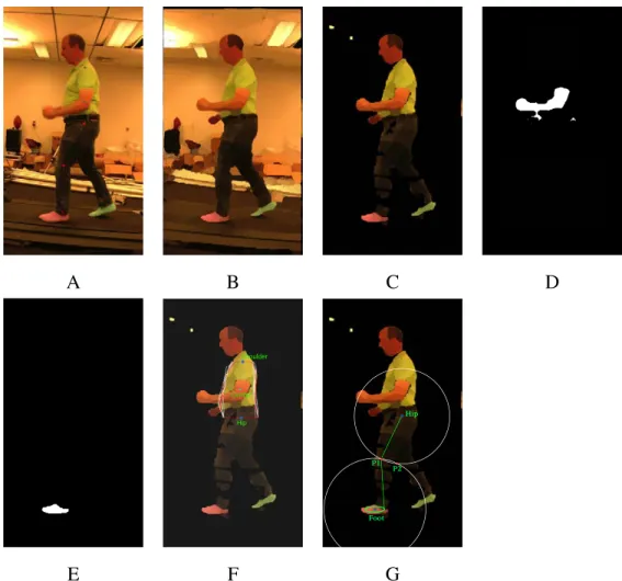
A B C D

E F G

Figure 3.5: (A) The subject walks on a treadmill with red markers placed on his body. (B) After applying [27], the edge information is enhanced, the color becomes more homogeneous and most noise is removed. (C) Background subtraction. (D) The skin extraction after removing face skin exposes the arm skin. (E) Foot color extraction. (F) The averaged torso shape is represented by a red curve, the white curves indicate the torso shape detected in each frame. The three points ("Center", "Shoulder", "Hip") are used to move and rotate the shape. (G) The knee position can be efficiently computed by intersecting two circles at P1 and P2.

Lastly, since the torso detection (shoulder and hip) plays an essential role in order to have successful arm and leg estimations, we also model the form of the subject’s main body in a way that minimizes the effect of his clothes on the final result. To facilitate processing as well as to increase robustness of our system, the bounding boxes are aligned along the horizontal axis, with respect to the first frame, to make sure that

the subject stays at the same location in all frames. The torso shape model is defined as <Lc, Rc> in which Lc= {xli, yli}Nc and Rc= {xri, yri}Nc are its left and right contours

respectively, Nc is the number of points of both Lc and Rc since they always have the

same scanline within the torso height ratio. Algorithm 1 demonstrates how to construct the Lk_c and Rk_c at frame k, note that we choose the top-left corner of the image as the origin coordinate.

Algorithm 1: Constructing the left and right contours of the torso model. Input: Subject silhouette after background subtraction at frame k Output: the contour model at frame k

1 Fill any black holes inside the silhouette

2 Define torso range [y_shoulder, y_hip] based on the torso height ratio 3 y← y_shoulder

4 while y > y_hipdo

5 Compute the center C of the current torso slice 6 (xk_li, yk_li) ← first background point on the left side of C 7 (xk_ri, yk_ri) ← first background point on the right side of C 8 Add (xk_li, yk_li) to Lk_c

9 Add (xk_ri, yk_ri) to Rk_c 10 y← y − 1

11 return < Lk_c, Rk_c >

To cope with the movement of clothes during a gait and arm occlusion, the final contour is calculated by averaging all contours < Lk_c, Rk_c > over the training frames, see Fig. 3.5(F). Given that the y-component is fixed, the x-component of the point at the i-th position of the final contour of Lcis computed as follows

x_lif inal = ∑

360

k (xkli∗ Ψkli)

360 − N_skinli (3.1)

where x_lik represents the value of x-coordinate of the i-th point of Lc at frame k, Ψk_li is

the binary function that gives 1 if the image point (xi, yi) at frame k is not skin point,

skin color. The final x-component of each element in Rc are deduced by using the same

formula. By the very similar manner, the x-component of the point at the i-th position of the final contour of Rc is computed as follows:

x_rif inal = ∑

360

k (xkri∗ Ψkri)

360 − N_skinri (3.2)

In essence, we want to minimize the effect of the swinging arm to the torso shape so whenever the arm intersects with either the left or right contour, the points within the intersection zone are not taken into account, as shown in the formula above. The torso model construction is computed over 360 frames. More details on how we use this model to accurately locate the position of shoulder and hip are explained in Section 3.3.1.

3.3 Pose estimation

In this section, we only explain our methodology for reconstructing the left half skeleton since the same process is executed on the right side. Firstly, the bounding box of the full person silhouette is extracted from the background subtraction result Isilhouette,

the relative height ratio between body parts is applied to divide this bounding box into sub-part bounding boxes obtained from anthropometry data [50]. We then estimate the orientation of arm, leg, head and the torso region. Finally, starting from the torso, the exact locations of head, arm and leg are inferred accordingly. This process ensures that we always obtain the model with stable relative position between body parts, one wrong estimated position of one node does not break the whole model. For example, in case of a bad estimated position of the shoulder, it only affects the angle between torso and upper arm, but not the angle between upper arm and lower arm.

3.3.1 Head and torso

An ellipse-based fitting technique [69], which is described below, is used for locating the head. The orientation of the main axis of the ellipse is the orientation of the head joint in our skeleton model. With known head length, we can easily locate the joints P_{f orehead}and Pchin along the main axis.

In order to perform the ellipse fitting efficiently on a set of scattered points, we use the well-known technique introduced in [69] which is fast and non-iterative, see Fig.3.6. In [69], a general conic can be represented by an implicit second order polynomial

f(a, x) = a₀x2+ a₁xy+ a₂y2+ a₃x+ a₄y+ a₅= a · x (3.3) where a = ( a0 a1 a2 a3 a4 a5)T and x = ( x2 xy y2 x y 1)T .

In the definition above, f (a, x) = 0 is the equation of the conic, and f (a, xi) is the

difference from point pi = (xi, yi) to the curve. The ellipse fitting can be stated as the

minimization of the sum of algebraic squared distances

d(a) =

N

∑

i=1

f2(a, xi) (3.4)

The N input points are gathered in the form of a design matrix D = [ x1 x2 · · · xN]T .

The objective function d(a) is then re-written as

d(a) = aTSa (3.5)

where S is the 6×6 scatter matrix. They make use of the equality constraint 4a0a2−a2₁=

1, or, in matrix form

aTCa = 1 (3.6)

where C is the constraint matrix. By introducing the Lagrange multiplier3λ and differ-entiating, they have to solve an eigen system subject to the constraint 3.6 as

Sa = λ Ca (3.7)

Since S is positive definite, there is a unique solution for the best fit ellipse. After finding the ellipse parameters, then positions, orientation, etc., are finally deduced. More details and mathematical proofs can be found in [69].

3. In mathematical optimization, the method of Lagrange multipliers is a strategy for finding the local maxima and minima of a function subject to equality constraints.