HAL Id: inria-00602205
https://hal.inria.fr/inria-00602205v2
Submitted on 26 Apr 2012
HAL is a multi-disciplinary open access
archive for the deposit and dissemination of
sci-entific research documents, whether they are
pub-lished or not. The documents may come from
teaching and research institutions in France or
L’archive ouverte pluridisciplinaire HAL, est
destinée au dépôt et à la diffusion de documents
scientifiques de niveau recherche, publiés ou non,
émanant des établissements d’enseignement et de
recherche français ou étrangers, des laboratoires
The Cosparse Analysis Model and Algorithms
Sangnam Nam, Mike E. Davies, Michael Elad, Rémi Gribonval
To cite this version:
Sangnam Nam, Mike E. Davies, Michael Elad, Rémi Gribonval.
The Cosparse Analysis Model
and Algorithms. Applied and Computational Harmonic Analysis, Elsevier, 2013, 34 (1), pp.30–56.
�10.1016/j.acha.2012.03.006�. �inria-00602205v2�
The Cosparse Analysis Model and Algorithms
✩S. Nama, M. E. Daviesb, M. Eladc, R. Gribonvala a
Centre de Recherche INRIA Rennes - Bretagne Atlantique, Campus de Beaulieu, F-35042 Rennes, France
bSchool of Engineering and Electronics, The University of Edinburgh, Edinburgh, EH9 3JL,
UK
c
Department of Computer Science, The Technion, Haifa 32000, Israel
Abstract
After a decade of extensive study of the sparse representation synthesis model, we can safely say that this is a mature and stable field, with clear theoretical foundations, and appealing applications. Alongside this approach, there is an
analysis counterpart model, which, despite its similarity to the synthesis
alter-native, is markedly different. Surprisingly, the analysis model did not get a similar attention, and its understanding today is shallow and partial.
In this paper we take a closer look at the analysis approach, better define it as a generative model for signals, and contrast it with the synthesis one. This work proposes effective pursuit methods that aim to solve inverse prob-lems regularized with the analysis-model prior, accompanied by a preliminary theoretical study of their performance. We demonstrate the effectiveness of the analysis model in several experiments, and provide a detailed study of the model associated with the 2D finite difference analysis operator, a close cousin of the TV norm.
Keywords: Synthesis, Analysis, Sparse Representations, Union of Subspaces, Pursuit Algorithms, Greedy Algorithms, Compressed-Sensing.
✩This work was supported in part by the EU through the project SMALL (Sparse Models,
Algorithms and Learning for Large-Scale data), FET-Open programme, under grant number: 225913
✩✩Some part of this work has been presented in a conference paper [38].
Email addresses: [email protected](S. Nam), [email protected] (M. E. Davies), [email protected] (M. Elad), [email protected] (R. Gribonval)
1. Introduction
Situated at the heart of signal and image processing, data models are fun-damental for stabilizing the solution of inverse problems, and enabling various other tasks, such as compression, detection, separation, sampling, and more. What are those models? Essentially, a model poses a set of mathematical prop-erties that the data is believed to satisfy. Choosing these propprop-erties (i.e. the model) carefully and wisely may lead to a highly effective treatment of the signals in question and consequently to successful applications.
Throughout the years, a long series of models has been proposed and used, exhibiting an evolution of ideas and improvements. In this context, the past decade has been certainly the era of sparse and redundant representations, a novel synthesis model for describing signals [5, 19, 36, 51]. Here is a brief description of this model:
Assume that we are to model the signal x ∈ Rd. The sparse and redundant synthesis model suggests that this signal could be described as x = Dz, where D∈ Rd×n is a possibly redundant dictionary (n ≥ d), and z ∈ Rn, the signal’s representation, is assumed to be sparse. Measuring the cardinality of non-zeros of z using the ‘ℓ0-norm’, such that kzk0 is the count of the non-zeros in z, we
expect kzk0to be much smaller than n. Thus, the model essentially assumes that
any signal from the family of interest could be described as a linear combination of few columns from the dictionary D. The name “synthesis” comes from the relation x = Dz, with the obvious interpretation that the model describes a way to synthesize a signal.
This model has been the focus of many papers, studying its core theoretical properties by exploring practical numerical algorithms for using it in practice (e.g. [9, 10, 11, 37]), evaluating theoretically these algorithms’ performance guarantees (e.g. [2, 15, 28, 54, 55]), addressing ways to obtain the dictionary from a bulk of data (e.g. [1, 23, 34, 47]), and beyond all these, attacking a long series of applications in signal and image processing with this model, demonstrating often state-of-the-art results (e.g. [20, 22, 32, 42]). Today, after a decade of an extensive study along the above lines, with nearly 4000 papers1
written on this model and related issues, we can safely say that this is a mature and stable field, with clear theoretical foundations, and appealing applications. Interestingly, the synthesis model has a “twin” that takes an analysis point of view. This alternative assumes that for a signal of interest, the analyzed vector Ωxis expected to be sparse, where Ω ∈ Rp×d is a possibly redundant analysis
operator (p ≥ d). Thus, we consider a signal as belonging to the analysis model
if kΩxk0 is small enough. Common examples of analysis operators include:
the shift invariant wavelet transform ΩWT [36]; the finite difference operator
ΩDIF, which concatenates the horizontal and vertical derivatives of an image
1
This is a crude estimate, obtained using ISI-Web-of-Science. By first searching Topic=(sparse and representation and (dictionary or pursuit or sensing)), 240 papers are obtained. Then we consider all the papers that cite the above-found, and this results with ≈3900 papers.
and is closely connected to total variation [45]; the curvelet transform [48], and more. Empirically, analysis models have been successfully used for a variety of signal processing tasks [24, 30, 48, 49, 50] such as denoising, deblurring, and most recently compressed sensing, but this has been done with little theoretical justification.
It is well known by now [21] that for a square and invertible dictionary, the synthesis and the analysis models are the same with D = Ω−1. The models remain similar for more general dictionaries, although then the gap between them is unexplored. Despite the close-proximity between the two—synthesis and analysis—models, the first has been studied extensively while the second has been left aside almost untouched. In this paper we aim to bring justice to the analysis model by addressing the following set of topics:
1. Cosparsity: In Section 2 we start our discussion with a closer look at the sparse analysis model in order to better define it as a generative model for signals. We show that, while the synthesis model puts an emphasis on the non-zeros of the representation vector z, the analysis model draws its strength from the zeros in the analysis vector Ωx.
2. Union of Subspaces: Section 2 is also devoted to a comparison between the synthesis model and the analysis one. We know that the synthesis model described above is an instance of a wider family of models, built as a finite union of subspaces [33]. By choosing all the sub-groups of columns from D that could be combined linearly to generate signals, we get an exponentially large family of low-dimensional subspaces that cover the signals of interest. Adopting this perspective, the analysis model can obtain a similar interpretation. How are the two related to each other? Section 2 considers this question and proposes a few answers.
3. Uniqueness: We know that the spark of the dictionary governs the uniqueness properties of sparse solutions of the underdetermined linear system Dz = x [15]. Can we derive a similar relation for the analysis case? As a platform for studying the analysis uniqueness properties, we consider an inverse problem of the form y = Mx, where M ∈ Rm×d and
m < d, and y ∈ Rm is a measurement vector. Put roughly (and this will
be better defined later on), assuming that x comes from the sparse anal-ysis model, could we claim that there is only one possible solution x that can explain the measurement vector y? Section 3 presents this uniqueness study.
4. Uniqueness: Worked Examples. Based on the study of the analysis uniqueness properties, we characterize the required number of measure-ments for the uniqueness of the signal that satisfies the analysis model in the case of analysis operator Ω in general position and the 2D one-step finite difference operator ΩDIF.
5. Pursuit Algorithms: Armed with a deeper understanding of the anal-ysis model, we may ask how to efficiently find x for the above-described linear inverse problem. As in the synthesis case, we can consider either relaxation-based methods or greedy ones. In Section 4 we present two
numerical approximation algorithms: a greedy algorithm termed “Greedy Analysis Pursuit” (GAP) that resembles the Orthogonal Matching Pur-suit (OMP) [37]—adapted to the analysis model—, and the previously considered ℓ1-minimization approach [7, 21, 46]. Section 5 accompanies
the presentation of GAP with a theoretical study of its performance guar-antee, deriving a condition that resembles the ERC obtained for OMP [54]. Similarly, we study the terms of success of the ℓ1-minimization
ap-proach for the analysis model, deriving a condition that is similar to the one obtained for the synthesis sparse model [54].
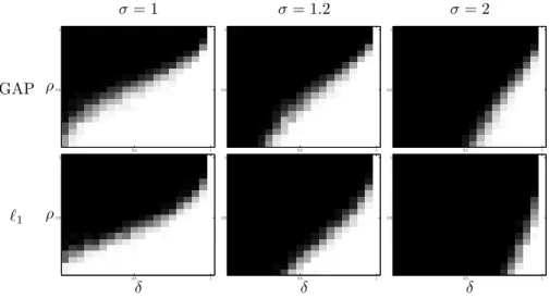
6. Tests: In Section 6 we demonstrate the effectiveness of the analysis model and the pursuit algorithms proposed in several experiments, starting from synthetic ones (involving random analysis operators) and going all the way to a compressed-sensing test for an image based on the analysis model: the Shepp Logan phantom.
We believe that with the above set of contributions, the cosparse analysis model becomes a well-defined and competitive model to the synthesis counterpart, equipped with all the necessary ingredients for its practical use. Furthermore, this work leads to a series of new questions that are parallel to those studied for the synthesis model—developing novel pursuit methods, a theoretical study of pursuit algorithms for handling other inverse problems, training Ω just as done for D, and more. We discuss these and other topics in Section 7.
Related Work. Several works exist in the literature that are related to the
anal-ysis model. The work by Elad et. al. [21] was the first to observe the dichotomy of analysis and synthesis models for signals. Their study, done in the context of the Maximum-A-Posteriori Probability estimation, presented the two alter-natives and explored cases of equivalence between the two. They demonstrated a superiority of the analysis-based approach in signal denoising. Further empir-ical evidence of the effectiveness of the analysis-based approach for signal and image restroation can be found in [43] and [46]. In [46] it was noted that the nonzero coefficients play a different role in the analysis and synthesis forms but the importance of the zero coefficients for the analysis model—which is reminis-cent of signal characterizations through the zero-crossings of their undecimated wavelet transform [35]—was not explicitly identified.
More recently, Cand`es et al. [7] provided a theoretical study on the error when the analysis-based ℓ1-minimization is used in the context of compressed
sensing. Our work is closely related to these contributions in various ways, and we shall return to these papers when diving into the details of our study.
2. A Closer Look at the Cosparse Analysis Model
We start our discussion with the introduction of the sparse analysis model, and the notion of cosparsity that is fundamental for its definition. We also describe how to interpret the analysis model as a generative one (just like the synthesis counterpart). Finally, we consider the interpretation of the sparse
analysis and synthesis models as two manifestations of union-of-subspaces mod-els, and show how they are related.
2.1. Introducing Cosparsity
As described in the introduction, a conceptually simple model for data would be to assume that each signal we consider can be expressed (i.e., well-approximated) as a combination of a few building atoms. Once we take this view, a simple synthesis model can be thought of: First, there is a collection of the atomic signals {dj}nj=1 ∈ Rd that we concatenate as the columns of a
dictionary, denoted by D ∈ Rd×n. Here, typically n ≥ d, implying that the
dictionary is redundant. Second, the signal x ∈ Rd can be expressed as a linear
combination of some atoms of D, thus there exists z ∈ Rn such that x = Dz.
Third and most importantly, x must lie in a low dimensional subspace, and in order to ensure this, very few atoms are used in the expression x = Dz, i.e., the number of non-zeros kzk0is very small. By the observation that kzk0 is small,
we say that x has a sparse representation in D. The number k = kzk0 is the
sparsity of the coefficient vector z and, by extension, of the signal x.
Often, the validity of the above described sparse synthesis model is demon-strated by applying a linear transform to a class of signals to be processed and observing that most of the coefficients are close to zero, exhibiting sparsity. In signal and image processing, discrete transforms such as wavelet, Gabor, curvelet, contourlet, shearlet, and others [14, 31, 36, 48], are of interest, and this empirical observation seems to give a good support for the sparse syn-thesis model. Indeed, when aiming to claim optimality of a given transform, this is exactly the approach taken – show that for a (theoretically-modeled) class of signals of interest, the transform coefficients tend to exhibit a strong decay. However, one cannot help but noticing that this approach of validat-ing the synthesis model seems to actually validate another ‘similar’ model; we are considering a model where the signals of interest have sparse analysis
rep-resentations. This point is especially pronounced when the transform used is
over-complete or redundant.
Let us now look more carefully at the above mentioned model that seems to be similar to the sparse synthesis one. First, let Ω ∈ Rp×d be a signal
transformation or an analysis operator. Its rows are the row vectors {ωj}pj=1
that will be applied to the signals. Applying Ω to x, we obtain the (analysis) representation Ωx of x. To capture various aspects of the information in x, we typically have p ≥ d.
For simplicity, unless stated otherwise, we shall assume hereafter that all the
rows of Ω are in general position, i.e., there are no non-trivial linear depen-dencies among the rows.2 Note that this assumption is used for the purpose of
contrasting the analysis model to the synthesis model, and that we will study a case when Ω is not in general position in later sections. As a matter of fact,
2Put differently, we assume that the spark of the matrix ΩT is full, implying that every
there is some indication that linear dependecies among the rows of Ω can be a ‘blessing.’ (See, e.g., uniqueness results in Sections 3.3 and 3.4.)
Clearly, unless x = 0, no representation Ωx can be ‘very sparse’, since at least p − d of the coefficients of Ωx are necessarily non-zeros. We shall put our emphasis on the number of zeros in the representation, a quantity we will call
cosparsity.
Definition 1. The cosparsity of a signal x ∈ Rd with respect to Ω ∈ Rp×d (or simply the cosparsity of x) is defined to be:
Cosparsity : ℓ := p − kΩxk0 (1)
The index set of the zero entries of Ωx is called the cosupport of x. We say that xhas cosparse representation or x is cosparse when the cosparsity of x is large, where by large we mean that ℓ is close to d. We will see that, while ℓ ≤ d for an analysis operator in general position, there are specific examples where ℓ may exceed d.
At first sight the replacement of sparsity by cosparsity might appear to be mere semantics. However we will see that this is not the case. In the synthesis model it is the columns dj, j ∈ T associated with the index set T of nonzero
coefficients that define the signal subspace. Removing columns from D not in T leaves this subspace unchanged. In contrast, it is the rows ωj associated with
the index set Λ such that hωj, xi = 0, j ∈ Λ that define the analysis subspace.
In this case removing rows from Ω for which hωj, xi 6= 0 leaves the subspace
unchanged.
From this perspective, the cosparse model is more related to signal charac-terizations from the zero-crossings of their undecimated wavelet transform [35] than to sparse wavelet expansions.
2.2. Sparse Analysis Model as a Generative Model
In a Bayesian context, one can think of data models as generators for random signals from a pre-specified probability density function. In that context, the signals that satisfy the k-sparse synthesis model can be generated as follows: First, choose k distinct columns of the dictionary D at random (e.g. assuming a uniform probability). We denote the index set chosen by T , and clearly |T | = k. Second, form a coefficient vector z that is k-sparse, with zeros outside the support T . The k non-zeros in z can be chosen at random as well (e.g. Gaussian iid entries). Finally, the signal is created by multiplying D to the resulting sparse coefficient vector z.
Could we adopt a similar view for the cosparse analysis model? The answer is positive. Similar to the above, one can produce an ℓ-cosparse signal in the following way: First, choose ℓ rows of the analysis operator Ω at random, and those are denoted by an index set Λ (thus, |Λ| = ℓ). Second, form an arbitrary signal v in Rd—e.g., a random vector with Gaussian iid entries. Then, project
v onto the orthogonal complement of the subspace generated by the rows of Ω that are indexed by Λ, this way getting the cosparse signal x. Explicitly,
x= (Id − ΩTΛ(ΩΛΩTΛ)−1ΩΛ)v. Alternatively, one could first find a basis for the
orthogonal complement and then generate a random coefficient vector for the basis.
This way, both models can be considered as generators of signals that have a special structure, and clearly, the two signal generators are different. It is now time to ask how those two families of signals inter-relate. In order to answer this question, we take the union-of-subspaces point of view.
2.3. Union-of-Subspaces Models
It is well known that the sparse synthesis model is a special instance of a wider family of models called union-of-subspaces [4, 33]. Given a dictionary D, a vector z that is exactly k-sparse with support T leads to a signal x = Dz = DTzT, a linear combination of k columns from D. The notation DT denotes
the sub-matrix of D containing only the columns indexed by T . Denoting the subspace spanned by these columns by VT := span(dj, j ∈ T ), the sparse
synthesis signals belong to the union of all¡n
k¢ possible subspaces of dimension
k,
Sparse Synthesis Model: x∈ ∪T :|T |=k VT. (2)
Similarly, the analysis model is associated to a union of subspaces model as well. Given an analysis operator Ω, a signal that is exactly ℓ-cosparse with respect to the rows Λ from Ω is simply in the orthogonal complement to these ℓ rows. Thus, we have3 Ω
Λx = 0, which implies that x ∈ WΛ, where WΛ :=
span(ωj, j ∈ Λ)⊥ = {x, hωj, xi = 0, ∀j ∈ Λ}. Put differently, we may write
WΛ = Range(ΩTΛ)⊥ = Null(ΩΛ). Hence, cosparse analysis signals x belong to
the union of all the¡p
ℓ¢ possible such subspaces of dimension d − ℓ,
Cosparse Analysis Model: x∈ ∪Λ:|Λ|=ℓ WΛ. (3)
The following table summarizes these two unions of subspaces, where we recall that we assume Ω and D in general position.
Model Subspaces No. of Subspaces Subspace dimension
Synthesis VT := span(dj, j ∈ T ) ¡nk¢ k
Analysis WΛ:= span(ωj, j ∈ Λ)⊥ ¡pℓ¢ d − ℓ
What is the relation between these two union of subspaces, as described in Equations (2) and (3)? In general, the answer is that the two are different. An interesting way to compare the two models is to consider an ℓ-cosparse analysis model and a corresponding (d − ℓ)-sparse synthesis model, so that the two have the same dimension in their subspaces.
3
Note that the notation ΩΛ refers to restricting rows from Ω indexed by Λ, whereas in
the synthesis case we have taken the columns. We shall use this convention throughout this paper, where from the context it should be clear whether rows or columns are extracted.
Following this guideline, we consider first a special case where ℓ = d − 1. In such a case, the dimension of the analysis subspaces is d − ℓ = 1, and there are ¡p
ℓ¢ of those. An equivalent synthesis union of subspaces can be created, where
k = 1. We should construct a dictionary D with n = ¡p ℓ
¢
atoms dj, where
each atom is the orthogonal complement to one of the sets of ℓ rows from Ω. While the two models become equivalent in this case, clearly n ≫ p in general, implying that the sparse synthesis model becomes intractable since D becomes too large.
By further assuming that p = d, we get that there are exactly¡p ℓ¢ = ¡
d
d−1¢ =
d subspaces in the analysis union, and in this case n = p = d as well. Further-more, it is not hard to see that in this case the synthesis atoms are obtained directly by a simple inversion, D = Ω−1.
Adopting a similar approach, considering the general case where ℓ is a general value (and not necessarily d − 1), one could always construct a synthesis model that is equivalent to the analysis one. We can compose the synthesis dictionary by simply concatenating all the bases for the orthogonal complements to the subspaces WΛ. The obtained dictionary will have at most (d − ℓ)¡pℓ¢ atoms.
However, not all supports of size k are allowed in the obtained synthesis model, since otherwise the new sparse synthesis model will strictly contain the cosparse analysis one. As such, the cosparse analysis model may be viewed as a sparse synthesis model with some structure.
Further on the comparison between the two models, it would be of benefit to consider again the case d − ℓ = k (i.e., having the same dimensionality), assume that p = n (i.e., having the same overcompleteness, for example with Ω = DT),
and compare the number of subspaces amalgamated in each model. For the sake of simplicity we consider a mild overcompleteness of p = n = 2d. Denoting H(t) := −t log2t − (1 − t) log2(1 − t), 0 < t < 1, the number of subspaces of
low dimension k ≪ d = n/2 in each data model, from Stirling’s approximation, roughly satisfies for large d:
Synthesis: log2 µn k ¶ ≈ n · Hµ kn ¶ ≈ k · log2 n k Analysis: log2 µp ℓ ¶ ≈ n · Hµ d − kn ¶ ≈ n · H(0.5) = n.
More generally, unless d/n ≈ 1, there are far fewer low-dimensional synthesis
subspaces than there are analysis subspaces of the same dimension. This is
illustrated on Figure 2.3 when n = p = 2d. This indicates a strong difference in the structure of the two models: The synthesis model includes very few low-dimensional subspaces, and an increasingly large number of subspaces of higher dimension, whereas the analysis model contains a combinatorial number of low-dimensional subspaces, with fewer high dimensional subspaces.
Comment: One must keep in mind that the huge number of low-dimensional subspaces, though rich in terms of its descriptive power, makes it very difficult to recover algorithmically signals that belong to the union of those low-dimensional subspaces or to efficiently code/sample those signals (see the experimental
re-0 0.1 0.2 0.3 0.4 0.5 0.6 0.7 0.8 0.9 1 0 0.2 0.4 0.6 0.8 1 k/d lo g2 (♯ su b p a c e s) / d
Number of subspaces of dimension k in Rd
Synthesis model, n/d=2 Analysis model, p/d =2 l=d−k
Figure 1: Number of subspaces of a given dimension, for n = p = 2d. The solid blue curve shows the log number of subspaces for the synthesis model as the dimension of subspaces vary, while the dashed red curve shows that for the analysis model.
sults in Section 6.1). This stems from the fact that, in general, it is not possible to get cosparsity d ≤ ℓ < p: any vector x that is orthogonal to d linearly inde-pendent rows of Ω must be the zero vector, leading to an uninformative model. One may, however, get cosparsities in the range d ≤ ℓ < p when the analysis operator Ω displays certain linear dependencies. Therefore it appears to be de-sirable, in the cosparse analysis model, to have analysis operators that exhibit high linear dependencies among their rows. We will see in Section 3.4 that a leading example of such operators is the finite difference analysis operator.
Another interesting point of view towards the difference between the two models is the following: While a synthesis signal is characterized by the support of the non-zeros in its representation in order to define the subspace it belong to, a signal from the analysis model is characterized by the locations of the zeros in its representation Ωx. The fact that this representation may contain many non-zeroes (and especially so when p ≫ d) should be of no consequence to the efficiency of the analysis model.
2.4. Comparison with the Traditional Sparse Analysis model
Previous work using analysis representations, both theoretical and algorith-mic, has focussed on gauging performance in terms of the more traditional sparsity perspective. For example, in the context of compressed sensing, recent theoretical work [7] has provided performance guarantees for minimum ℓ1-norm
analysis representations in this light.
The analysis operator is generally viewed as the dual frame for a redundant synthesis dictionary so that Ω = D†. This means that the analysis coefficients
Ωxprovide a consistent synthesis representation for x in terms of the dictionary D, implying that the representation Ωx is a feasible solution to the linear system of equations Dz = x.
synthesis model,S T :|T |=kVT, with k = p − ℓ. Hence: {0} ⊆ [ Λ:|Λ|=p−k WΛ⊆ [ T :|T |=k VT ⊆ Rd. (4)
Of course, Ωx is not guaranteed to be the sparsest representation of x in terms of D. Hence the two subspace models are not equivalent.
Note that while in Section 2.3 the sparsity k was matched to d − ℓ, here it is matched to p − ℓ. The former was used to get the same dimensions in the resulting subspaces, while the match discussed here considers the vector Ωx as a candidate k-sparse representation.
Such a perspective treats the analysis operator as a poor man’s sparse syn-thesis representation. That is, for certain signals x, the representation Ωx may be reasonably sparse but is unlikely to be as sparse as, for example, the minimum ℓ1-norm synthesis representation4.
In the context of linear inverse problems, it is tempting to try to exploit the nesting property (4) in order to derive identifiability guarantees in terms of the sparsity of the analysis coefficients Ωx. For example, in [7], the compressed sensing recovery guarantees exploit the nesting property (4) by assuming a suffi-cient number of observations to achieve a stable embedding (restricted isometry property) for the k-sparse synthesis union of subspaces, which in turn implies a stable embedding of the (p − k)-cosparse analysis union of subspaces.
While such an approach is of course valid, it misses a crucial difference between the analysis and synthesis representations: they do not correspond to equivalent signal models. Treating the two models as equivalent hides the fact that they may be composed of subspaces with markedly different dimensions. The difference between these models is highlighted in the following examples.
2.4.1. Example: generic analysis operators, p = 2d
Assuming the rows of Ω are in general position, then when p ≥ 2d the nesting property (4) is trivial but rather useless! Indeed, if k < d, then the only analysis signal for which kΩxk0 = k = p − ℓ is x = 0. Alternatively, if k ≥ d,
the synthesis model is trivially the full space: S
T :|T |=kVT = Rd.
2.4.2. Example: shift invariant wavelet transform
The shift invariant wavelet transform is a popular analysis transform in signal processing. It is particularly good for processing piecewise smooth signals. Its inverse transform has a synthesis interpretation as the redundant wavelet dictionary consisting of wavelet atoms with all possible shifts.
The shift invariant wavelet transform [36] provides a nice example of an analysis operator that has significant dependencies due to the finite support of
4
When measuring sparsity with an ℓpnorm, 0 < p ≤ 1, rather than with p = 0, it has been
shown [29] that for so-called localized frames the analysis coefficients Ωx obtained with Ω = D† the canonical dual frame of D are near optimally sparse: kΩxkp≤ Cpminz|Dz=xkzkp,
the individual wavelets. Such nontrivial dependencies within the rows of ΩWT
mean that the dimensions of the (analysis or synthesis) signal subspaces are not easily characterised by either the sparsity k or the cosparsity ℓ. However the behaviour of the model is still driven by the zero coefficients not the nonzero ones, i.e., by the zero-crossings of the wavelet transform [35]. By considering a particular support set of an analysis representation ΩWTx with the shift
invariant wavelet transform we can illustrate the dramatic difference between the analysis and synthesis interpretations of the coefficients.
20 40 60 80 100 120 1
2
3
4
Figure 2: Top: a piecewise quadratic signal. Bottom: the support set (white region) for the wavelet coefficients of the signal using a J = 4 level shift invariant Daubechies wavelet transform with s = 3 vanishing moments. Scaling coefficients are not shown. The support set contains 122 coefficients out of a possible 512, yet the analysis subspace has a dimension of only 3.
Figure 2 shows the support set of the nonzero analysis coefficients (white re-gion), associated with the cone of influence around a discontinuity in a piecewise polynomial signal of length 128-samples [18], using a shift-invariant Daubechies wavelet transform with s = 3 vanishing moments [36]. For such a signal, the cone of influence at level J in a shift invariant wavelet transform contains Lj−1
nonzero coefficients where Lj is the length of the wavelet filter at level j. Note
though, the nonzero coefficients are not linearly independent and can be ele-gantly described through the notion of wavelet footprints [18].
Synthesis perspective. Interpreting the support set within the synthesis model implies that the signal is not particularly sparse and needs a significant number of wavelet atoms to describe it: in Figure 2 the size of the support set, excluding coefficients of scaling functions, is 122. Could the support set be significantly reduced by using a better support selection strategy such as ℓ1
minimization? In practice, using ℓ1 minimization, a support set of 30 can be
obtained, again ignoring scaling coefficients.
Analysis perspective. The analysis interpretation of the shift invariant wavelet representation relies on the examination of the size of the analysis sub-space associated with the cosupport set. From the theory of wavelet footprints, the dimension of this subspace is equal to the number of vanishing moments of the wavelet filter, which in this example is only . . . 3, providing a much lower dimensional signal model.
We therefore see that the analysis model has a much lower number of degrees of freedom for this support set, leading to a significantly more parsimonious
model.
2.5. Hybrid Analysis/Synthesis models?
In this section we have demonstrated that while both the cosparse analysis model and the sparse synthesis model can be described by a union of subspaces these models are typically very different. We do not argue that one is inevitably better than the other. The value of the model will very much depend on the problem instance. Indeed the intrinsic difference between the models also sug-gests that it might be fruitful to explore building other union of subspace models from hybrid compositions of analysis and synthesis operators. For example, one could imagine a signal model where x = Dz through a redundant synthesis dictionary but instead of imposing sparsity on z we restrict z through an ad-ditional analysis operator: kΩzk0 ≤ k. In such a case there will still be an
underlying union of subspace model but with the subspaces defined by a combi-nation of atoms and analysis operator constraints. A special case of this is the split analysis model suggested in [7].
3. Uniqueness Properties
In the synthesis model, if a dictionary D is redundant, then a given signal x can admit many synthesis representations ˜z, i.e., ˜zwith D˜z= x. This makes the following type of problem interesting in the context of the sparse signal recovery: When a signal has a sparse representation z, can there be another representation that is equally sparse or sparser? This problem is well-understood in terms of the so-called spark of D [15], the smallest number of columns from D that are linearly dependent.
Unlike in the synthesis model, if the signal is known, then its analysis repre-sentation Ωx with respect to an analysis operator Ω is completely determined. Hence, there is no inherent question of uniqueness for the cosparse analysis model. The uniqueness question we want to consider in this paper is in the context of the noiseless linear inverse problem,
y= Mx, (5)
where M ∈ Rm×d, and m < d, implying that the measurement vector y ∈ Rmis
not sufficient to fully characterize the original signal x ∈ Rd. For this problem we
ask: when can we assert that a solution x with cosparsity ℓ is the only solution with that cosparsity or more? The problem (5) (especially, with additive noise) arises ubiquitously in many applications, and we shall focus on this problem throughout this paper as a platform for introducing the cosparse analysis model, its properties and behavior. Not to complicate matters unnecessarily, we assume that all the rows of M are linearly independent, and we omit noise, leaving robustness analysis to further work.
For completeness of our discussion, let us return for a moment to the synthe-sis model and consider the uniqueness property for the inverse problem posed in Equation (5). Assuming that the signal’s sparse representation satisfies x = Dz,
we have that y = Mx = MDz. Had we known the support T of z, this linear system would have reduced to y = MDTzT, a system of m equations with k
unknowns. Thus, recovery of x from y is possible only if k ≤ m.
When the support of z is unknown, it is the spark of the compound ma-trix MD that governs whether the cardinality of zT is sufficient to ensure
uniqueness—if k = kzk0 is smaller than half the spark of MD, then
neces-sarily z is the signal’s sparsest representation. At best, Spark(MD) = m + 1, and then we require that the number of measurements is at least twice the cardinality k. Put formally, we require
k = kzk0<1
2Spark(MD) ≤ m + 1
2 . (6)
It will be interesting to contrast this requirement with the one we will derive hereafter for the analysis model.
3.1. Uniqueness When the Cosupport is Known
Before we tackle the uniqueness problem for the analysis model, let us con-sider an easier question: Given the observations y obtained via a measurement matrix M, and assuming that the cosupport Λ of the signal x is known, what are the sufficient conditions for the recovery of x? The answer to this question is straightforward since x satisfies the linear equation
·y 0 ¸ =· M ΩΛ ¸ x= Ax. (7)
To be able to uniquely identify x from Equation (7), the matrix A must have a zero null space. This is equivalent to the requirement
Null(ΩΛ) ∩ Null(M) = WΛ∩ Null(M) = {0}. (8)
Let us now assume that M and Ω are mutually independent, in the sense that there are no nontrivial linear dependencies among the rows of M and Ω; this is a reasonable assumption because first, one should not be measuring something that may be already available from Ω, and second, for a fixed Ω, mutual independency holds true for almost all M (in the Lebesgue measure). Then, (8) would be satisfied as soon as dim(WΛ) + dim(Null(M)) ≤ d, or
dim(WΛ) ≤ m, since dim(Null(M)) = d − m. This motivates us to define
κΩ(ℓ) := max
|Λ|≥ℓ dim(WΛ). (9)
The quantity κΩ(ℓ) plays an important role in determining the necessary
and sufficient cosparsity level for the identification of cosparse signals. Indeed, under the assumption of the mutual independence of Ω and M, a necessary and sufficient condition for the uniqueness of every cosparse signal given the knowledge of its cosupport Λ of size ℓ is
3.2. Uniqueness When the Cosupport is Unknown
The uniqueness question that we answered above refers to the case where the cosupport is known, but of course, in general this is not the case. We shall assume that we may only know the cosparsity level ℓ, which means that our uniqueness question now becomes: what cosparsity level ℓ guarantees that there can be only one signal x matching a given observation y?
As we have seen, the cosparse analysis model is a special case of a general union of subspaces model. Uniqueness guarantees for missing data problems such as (5) with general union of subspace models are covered in [4, 33]. In particular [33] shows that M is invertible on the union of subspaces ∪γ∈ΓSγ if
and only if M is invertible on all subspaces Sγ + Sθ for all γ, θ ∈ Γ. In the
context of the analysis model this gives the following result whose proof is a direct consequence of the results in [33]:
Proposition 2 ([33]). Let ∪ΛWΛ, |Λ| = ℓ be the union of ℓ-cosparse analysis
subspaces induced by the analysis operator Ω. Then the following statements are equivalent:
1. If the linear system y = Mx admits an ℓ-cosparse solution, then this is
the unique ℓ-cosparse solution;
2. M is invertible on ∪ΛWΛ;
3. (WΛ1+ WΛ2) ∩ Null(M) = 0 for any |Λ1|, |Λ2| ≥ ℓ;
Proposition 2 answers the question of uniqueness for cosparse signals in the context of linear inverse problems. Unfortunately, the answer we obtained still leaves us in the dark in terms of the necessary cosparsity level or necessary number of measurements. In order to pose a clearer condition, we use Propo-sition 2 from [33] that poses a sharp condition on the number of measurements to guarantee uniqueness (when M and Ω are mutually independent):
m ≥ ˜κΩ(ℓ), where ˜κΩ(ℓ) := max {dim(WΛ1+ WΛ2) : |Λi| ≥ ℓ, i = 1, 2}
(11) Interestingly, a sufficient condition can also be obtained using the quantity κΩ
defined in (9) above, which was observed to play an important role in the unique-ness result when the cosupport is assumed to be known. Namely, we have the following result.
Proposition 3. Assume that κΩ(ℓ) ≤ m2. Then for almost all M (wrt the
Lebesgue measure), the linear inverse problem y = Mx has at most one ℓ-cosparse solution.
Proof. Assuming the mutual independence of Ω and M, which holds for almost
all M, we note that the uniqueness of ℓ cosparse solutions holds if and only if: dim (WΛ1+ WΛ2) ≤ m, whenever |Λi| ≥ ℓ, i = 1, 2. Assume that κΩ(ℓ) ≤
m/2. By definition of κΩ, if |Λi| ≥ ℓ, i = 1, 2, then dim(WΛi) ≤ m
2, hence
In the synthesis model the degree to which columns are interdependent can be partially characterized by the spark of D [15] defined as the the smallest number of columns of D that are linearly dependent. Here the function κΩ
plays a similar role in quantifying the interdependence between rows in the analysis model.
Remark 4. The condition κΩ(ℓ) ≤ m2 is in general not necessary while
condi-tion (11) is.
There are two classes of analysis operators for which the function κΩ is well-understood: analysis operators in general position and the finite difference operators. We discuss the uniqueness results for these two classes in the follow-ing subsections.
3.3. Analysis Operators in General Position
It can be easily checked that κΩ(ℓ) = max(d − ℓ, 0). This enables us to quantify the exact level of cosparsity necessary for the uniqueness guarantees: Corollary 5. Let Ω ∈ Rp×dbe an analysis operator in general position. Then, for almost all m × d matrices M, the following hold:
• Based on Eq. (10), if m ≥ d − ℓ, then the equation y = Mx has at most
one solution with known cosupport Λ (of cosparsity at least ℓ);
• Based on Proposition 2, if m ≥ 2(d − ℓ), then the equation y = Mx has
at most one solution with cosparsity at least ℓ. 3.4. The Finite Difference Operator
An interesting class of analysis operators with significant linear dependencies is the family of finite difference operators on graphs, ΩDIF. These are strongly
related to TV norm minimization, popular in image processing applications [45], and has the added benefit that we are able to quantify the function κΩand hence
the uniqueness properties of the cosparse signal model under ΩDIF.
We begin by considering ΩDIF on an arbitrary graph before restricting our
discussion to the 2D lattice associated with image pixels. Consider a non-oriented graph with vertices V and edges E ⊂ V2. An edge e is a pair e = (v
1, v2)
of connected vertices. For any vector of coefficients defined on the vertices, x∈ RV, the finite difference analysis operator ΩDIFcomputes the collection of
differences (x(v1) − x(v2)) between end-points, for all edges in the graph. Thus,
an edge e ∈ E may be viewed as a finite difference on RV.
Can we estimate the function κΩDIF(ℓ)? The following shows that it is
intimately related to topological properties of the graph. For each sub-collection Λ ⊂ E of edges, we can define its vertex-set V (Λ) ⊂ V as the collection of vertices covered by at least one edge in Λ. The support set V (Λ) of Λ can be decomposed into J(Λ) connected components (a connected component is a set of vertices connected to one another by a walk through vertices in Λ). It is easy to check that a vector x belongs to the space WΛ= Null(ΩΛ) if and only if its
values are constant on each connected component. As a result, the dimension of this subspace is given by
dim(WΛ) = |V | − |V (Λ)| + J(Λ)
where the |V | − |V (Λ)| vertices out of V are associated to arbitrary values in x that are distinct from all their neighbors, while all entries from each of the J(Λ) connected components have an arbitrary common value. It follows that
κΩ(ℓ) = max |Λ|≥ℓ n |V | − |V (Λ)| + J(Λ)o= |V | − min |Λ|≥ℓ n |V (Λ)| − J(Λ)o (12)
Because of the nesting of the subspaces WΛ, the minimum on the right hand
side is achieved when |Λ| = ℓ.
Uniqueness Condition for Cosparse Images with respect to the 2D ΩDIF. In
the abstract context of general graphs, the characterization (12) may remain obscure, but can we get more concrete estimates by specializing to the 2D regular graph associated to the pixels of an N × N image? It turns out that one can obtain relatively simple upper and lower bounds for κΩDIF and hence derive
an easily interpretable uniqueness condition (see Appendix C for a proof): Proposition 6. Let ΩDIF be the 2D finite difference analysis operator that
computes horizontal and vertical discrete derivatives of a d = N × N image. For any ℓ we have
d −ℓ2−r ℓ2 − 1 ≤ κΩDIF(ℓ) ≤ d − ℓ 2 − r ℓ 2 + 1 2 (13)
As a result, assuming that M is ‘mutually independent’ from ΩDIF, and if
m ≥ 2d − ℓ −√2ℓ +1
2 ≥ 2κΩDIF(ℓ) (14)
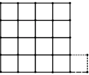
then the equation y = Mx has at most one solution with cosparsity at least ℓ. The 2D ΩDIF, Piecewise Constant Images, and the TV norm. The 2D finite
difference operator is closely related to the TV norm [45]: the discrete TV norm of x is essentially a mixed ℓ2− ℓ1 norm of ΩDIFx. Just like its close cousin TV
norm minimization, the minimization of kΩxk0is particularly good at inducing
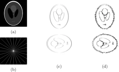
piecewise constant images. We illustrate this through a worked example. Consider the popular Shepp Logan phantom image shown in the left-hand side of Figure 3. We denote the cosupport of the image by Λ in line with the discussion in this section: An edge belongs to Λ if a pair of horizontally or vertically neighboring pixels v1 and v2 have the same value. This particular
image has 14 distinct connected regions of constant intensity. The number of non-zero coefficients in the finite difference representation is determined by the total length (Manhattan distance) of the boundaries between these regions. For the Shepp Logan phantom this length is 2546 pixel widths and thus the
cosparsity is ℓ = 130560 − 2546 = 128014. Furthermore, as there are no isolated pixels with any other intensity, all pixels belong to a constant intensity region so that |V (Λ)| = |V | and the cosupport has an associated subspace dimension of:
dim(WΛ) = (|V | − |V (Λ)|) + J(Λ)
= 14
Figure 3: Top left: an example of a piecewise constant image: the 256 × 256 Shepp Logan phantom; Top right: an image with the same cosparsity, ℓ = 128014, but whose cosupport is associated with an empirically maximum subspace dimension. Bottom: zoom on the top of the top right image.
In order to determine when the Shepp Logan image is the unique solution to y = Mx with maximum cosparsity it is necessary to consider the maximum subspace dimension of all possible support sets with the same cosparsity. This is the quantity measured by κΩDIF(ℓ).
Following the arguments used in the proof of Proposition 6 we need to find an image for which the ΩDIF cosupport, Λ, is a single connected subgraph that
is as close to a square as possible. Such an image is shown in the right hand side of Figure 3. For this image we have dim(WΛ) = 1276. Comparing this to
the bounds given in (13) of Proposition 6
1275 ≤ κΩDIF(ℓ) ≤ 1276,
we see that in this instance the upper bound has been achieved. The unique-ness result from Proposition 6 then tells us that a sufficient number of mea-surements to uniquely determine the Shepp Logan image is given by m = 2κΩDIF(128014) = 2552.
We will revisit this again in Subsection 6.2 where we investigate the empirical recovery performance of some practical reconstruction algorithms.
3.5. Overview of cosparse vs sparse models for inverse problems
To conclude this section, Figure 4 provides a schematic overview of analy-sis cosparse models vs syntheanaly-sis sparse models in the context of linear inverse problems such as compressed sensing. In the synthesis model, the signal x is
Figure 4: A schematic overview of analysis cosparse vs synthesis sparse models in relation with compressed sensing.
a projection (through the dictionary D) of a high-dimensional vector z living in the union of sparse coefficient subspaces; in the analysis model, the signal lives in the pre-image by the analysis operator Ω of the intersection between the range of Ω and this union of subspaces. For a given sparsity of z, this is usually a set of much smaller dimensionality.
4. Pursuit algorithms
Having a theoretical foundation for the uniqueness of the problem ˆ
x= arg min
x kΩxk0 subject to Mx = y, (15)
we now turn to the question of how to solve it: algorithms. We present two algorithms, both targeting the solution of problem (15). As in the uniqueness discussion, we assume that M ∈ Rm×d, where m < d. This implies that the
equation Mx = y has infinitely many possible solutions, and the term kΩxk0
introduces the analysis model to regularize the problem.
4.1. The Cosparse Signal Recovery Problem is NP-complete
Related to (15), we can consider a cosparse signal recovery problem COSPARSE consisting of a quintuplet (y, M, Ω, ℓ, ǫ) in which we seek to find a vector x∗
that satisfies
ky − Mx∗k
2≤ ǫ, kΩx∗k0≤ p − ℓ (16)
where p is the number of rows of Ω as before. It is easy to see that the decision problem “given (y, M, Ω, ℓ, ǫ), does there exist x∗satisfying (16)?” is NP [25]:
given a candidate solution, one can check in polynomial time whether it satisfies the constraints (16). Moreover, every instance of the classical NP-complete (ǫ, k) SPARSEapproximation problem [13, 40] can trivially be reduced to an instance of the above decision problem with Ω = Id, hence COSPARSE is indeed NP-complete.
The above consideration prompts us to look for ways to solve (15) in an ‘approximate’ way. We discuss two possibilities, a convex relaxation and a greedy approach, with an emphasis on the latter. Of course, there can be many more possibilities to solve (15) or to find approximate solutions of it. We mention a few works where some of such methods can be found: [6, 43, 46].
4.2. The Analysis ℓ1-minimization
A natural convex relaxation of (15) is to solve: ˆ
x= arg min
x kΩxk1 subject to Mx = y. (17)
The analysis ℓ1-minimization is well-known and widely used already in
prac-tice (see e.g. [22, 51]). The attractiveness of this approach comes from that the convexity of (17) admits computationally tractable algorithms to solve the problem, and that the ℓ1-norm promotes high cosparsity in the solution ˆx. An
algorithm that targets the solution of (17) and its convergence analysis can be found in [6]. There are many other papers that have introduced algorithms to solve problems of the form (17) or variants thereof. To give just an example, [44] proposes a general form of forward-backward splitting that can be exploited to deal with such problems.
4.3. The Greedy Analysis Pursuit Algorithm (GAP)
The algorithm we present in this section is named Greedy Analysis Pur-suit (GAP). It is a variant of well-known greedy purPur-suit algorithm used for the synthesis model—the Orthogonal Matching Pursuit (OMP) algorithm. Similar to the synthesis case, our goal is to detect the informative support of Ωx—as discussed in Section 3.1, in the analysis case, this amounts to the locations (co-support) of the zeros in the vector Ωx, so as to introduce additional constraints to the underdetermined system Mx = y. Note that for obtaining a solution, one needs to detect at least d−m of these zeros, and thus if ℓ > d−m, detection of the complete set of zeros is not mandatory.
An obvious way to find the cosupport of a cosparse signal would proceed as follows: First, obtain a reasonable estimate of the signal from the given information. Using the initial estimate, select a location as belonging to the cosupport. Having this estimated part of the cosupport, we can obtain a new estimate. One can now see that by alternating the two previous steps, we will have estimated enough locations of the cosupport to get the final estimate.
However, the GAP works in an opposite direction and aims to detect the elements outside the set Λ, this way carving its way towards the detection of the desired cosupport. Therefore, the cosupport ˆΛ is initialized to be the whole
set {1, 2, 3, . . . , p}, and through the iterations it is reduced towards a set of size ℓ (or less, d − m).
Let us discuss the algorithm with some detail. First, the GAP uses the following initial estimate:
ˆ
x0= arg min
x kΩxk
2
2 subject to y= Mx. (18)
Not knowing the locations of the cosupport but knowing that many entries of Ωx0 are zero, this is a reasonable first estimate of x0. Once we have ˆx0, we
can view Ωˆx0 as an estimate of Ωx0. Hence, we find the location of the largest
entries (in absolute value) of Ωˆx0 and regard them as not belonging to the
cosupport. After this, we remove the corresponding rows from Ω and work with a reduced Ω. A detailed description of the algorithm is given in Figure 5.
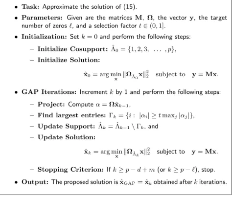
• Task: Approximate the solution of (15).
• Parameters: Given are the matrices M, Ω, the vector y, the target number of zeros ℓ, and a selection factor t ∈ (0, 1].
• Initialization: Set k = 0 and perform the following steps: – Initialize Cosupport: ˆΛ0= {1, 2, 3, . . . , p}, – Initialize Solution: ˆ x0= arg min x kΩΛ0ˆ xk 2 2 subject to y= Mx.
• GAP Iterations: Increment k by 1 and perform the following steps: – Project: Compute α = Ωˆxk−1,
– Find largest entries: Γk= {i : |αi| ≥ t maxj|αj|},
– Update Support: ˆΛk= ˆΛk−1\ Γk, and
– Update Solution: ˆ xk= arg min x kΩΛˆkxk 2 2 subject to y= Mx.
– Stopping Criterion: If k ≥ p − d + m (or k ≥ p − ℓ), stop. • Output: The proposed solution is ˆxGAP= ˆxkobtained after k iterations.
Figure 5: Greedy Analysis Pursuit Algorithm (GAP)
Some readers may notice that the GAP has similar flavors to the FOCUSS [26] and the IRLS [12]. This is certainly true in the sense that the GAP solves constrained least squares problems and adjusts weights as it iterates. However, the weight adjustment in the GAP is more aggressive (removal of rows) and binary in nature. We also note that the use of the selection factor t in the GAP is related to Weak Greedy Algorithms [53] for the synthesis model.
Stopping criterion / targeted sparsity. In GAP, we have a range of choices
be-tween using the full ℓ zeros in the product Ωx versus a minimal and sufficient set of d − m zeros. In between these two values, and assuming that the proper elements of Λ have been detected, we expect the solution obtained by the al-gorithms to be the same, with a slightly better numerical stability for a larger number of zeros.
Thus, an alternative stopping criterion for the GAP could be to detect whether the solution is static or the analysis coefficients of the solution are small. This way, even if the GAP made an error and removed from ˆΛk an index
that belongs to the true cosupport Λ, the tendency of the solution to stabilize could help in preventing the algorithm to incorporate this error into the solution. In fact, this criterion is used in the experiment in Section 6.
Multiple selections. The selection factor 0 < t ≤ 1 allow the selection of multiple
rows at once, to accelerate the algorithm by reducing the number of iterations.
Solving the required least squares problems. The solution of Eq. (18) (and of
the adjusted problems with reduced Ω at subsequent steps of the algorithm)— under some suitable conditions—is given analytically (see Appendix E for the derivation) by
ˆ
x0= (MTM+ (Id − MT(MMT)M)ΩTΩ)−1MTy. (19)
In practice, instead of (18), we compute
ˆ x0= arg min x ©ky − Mxk 2 2+ λkΩxk22ª = arg min x ° ° ° ° ·y 0 ¸ − · M √ λΩ ¸ x ° ° ° ° 2 2
for a small λ > 0, yielding the solution
ˆ x0= · M √ λΩ ¸† ·y 0 ¸ = (MTM+ λΩTΩ)−1MTy.
We point out that the use of the parameter λ is for convenience in this work but it becomes more useful when dealing with noisy observation. Furthermore, the small value of λ can have adverse effects on computational cost for some numerical algorithms (e.g., the conjugate gradient method) to solve the above minimization. In our implementation, we have used λ values roughly from 10−4
to 10−6.
5. Theoretical analysis
So far, we have introduced the cosparse analysis data model, provided unique-ness results in the context of linear inverse problems for the model, and described some algorithms that may be used to solve such linear inverse problems to re-cover cosparse signals. Before validating the algorithms and the model pro-posed with experimental results, we first investigate theoretically under what
conditions the proposed algorithms to solve cosparse signal recovery (15) are guaranteed to work. After that, we discuss the nature of the condition derived by contrasting it to that for the synthesis model. Further discussion including some desirable properties of Ω and M can be found in Appendix D.
5.1. A Sufficient Condition for the Success of the ℓ1-minimization
In the sparse synthesis framework, there is a well-known necessary and suf-ficient condition called the null space property (NSP) [16] that guarantees the success of the synthesis ℓ1-minimization
ˆ
z0:= argmin
z kzk
1 subject to y= Φz (20)
to recover the sparsest solution, say z0, to y = Φz. To elaborate, in the case
of a fixed support T , the ℓ1-minimization (20) recovers every sparse coefficient
vector z0 supported on T if and only if
kzTk1< kzTck1, ∀z ∈ Null(Φ), z 6= 0. (21)
The NSP (21) cannot easily be checked but some ‘simpler’ sufficient conditions can be derived from it; for example, one can get a recovery condition of [54] called the Exact Recovery Condition (ERC):
k|Φ†TΦTc|k
1→1< 1, (22)
where the notation k|A|kp→qdenotes the operator norm of A from ℓp to ℓq, i.e.,
k|A|kp→q:= sup x6=0
kAxkq
kxkp
.
The ERC (22) also implies the success of greedy algorithms such as OMP [54]. Note that here we used the symbol Φ for an object which may be viewed as a dictionary or a measurement matrix. Separating the data model and sampling, we can write Φ = MD as was done in Section 3.
One may naturally wonder: is there a condition for the cosparse analysis model that is similar to (21) and (22)? The answer to this question seems to be affirmative with some qualification as the following two results show (the proofs are in Appendix A):
Theorem 7. Let Λ be a fixed cosupport. The analysis ℓ1-minimization
ˆ
x0:= argmin
x kΩxk1
subject to y:= Mx0= Mx (23)
recovers every x0 with cosupport Λ as a unique minimizer if, and only if,
sup
xΛ:ΩΛxΛ=0
|hΩΛcz, sign(Ω
Λcx
Corollary 8.Let NT be any d×(d−m) basis matrix for the null space Null(M),
and Λ be a fixed cosupport such that the ℓ × (d − m) matrix ΩΛNT is of full
rank d − m. If
sup
xΛ:ΩΛxΛ=0
k(NΩTΛ)†NΩTΛcsign(ΩΛcxΛ)k∞< 1, (25)
then the analysis ℓ1-minimization (23) recovers every x0 with cosupport Λ.
Moreover, if
k|(NΩTΛ)†NΩTΛc|k∞→∞= k|ΩΛcNT(ΩΛNT)†|k1→1< 1 (26)
then condition (25) holds true.
There is an apparent similarity between the analysis ERC condition (26) above and its standard synthesis counterpart (22), yet there are some subtle differences between the two that will be highlighted in Section 5.3.
5.2. A Sufficient Condition for the Success of the GAP
There is an interesting parallel between the synthesis ERC (22) and its anal-ysis version in Corollary 8; namely, the analanal-ysis ERC condition (26) also implies the success of the GAP algorithm when the selection factor t of the GAP is 1 (in fact, k|ΩΛcNT(ΩΛNT)†|k1→1< t ≤ 1), as we will now show.
From the way GAP algorithm works, we can guarantee that it will perform a correct elimination at the first step if the largest analysis coefficients of ΩΛcxˆ0
of the first estimate ˆx0 are larger than the largest of ΩΛxˆ0 where Λ denotes
the true cosupport of x0. This observation suggests that we can hope to find
a condition for success if we can find some relation between ΩΛcxˆ
0 and ΩΛxˆ0.
The following result provides such a relation:
Lemma 9. Let NT be any d × (d − m) basis matrix for the null space Null(M)
and Λ be a fixed cosupport such that the ℓ × (d − m) matrix ΩΛNT is of full
rank d − m. Let a signal x0 with ΩΛx0 = 0 and its observation y = Mx0 be
given. Then the estimate ˆx0 in (18) satisfies
ΩΛxˆ0= −(NΩTΛ)†NΩTΛcΩΛcxˆ0. (27)
Having obtained a relation between ΩΛxˆ0 and ΩΛcxˆ0, we can derive a
suf-ficient condition which guarantees the success of GAP for recovering the true target signal x0:
Theorem 10. Let NT be any d×(d−m) basis matrix for the null space Null(M)
and Λ be a fixed cosupport such that the ℓ × (d − m) matrix ΩΛNT is of full
rank d − m. Let a signal x0 with ΩΛx0 = 0 and an observation y = Mx0 be
given. Suppose that the analysis ERC (26) holds true. Then, when applied to solve (15), GAP with selections factor t > k|(NΩT
Λ)†NΩTΛc|k∞→∞ will recover
Proof. At the first iteration, GAP is doing the correct thing if it removes a row
from ΩΛc. Clearly, this happens when
kΩΛxˆ0k∞< tkΩΛcˆx0k∞. (28)
In view of (27), if (26) holds and t > k|(NΩT
Λ)†NΩTΛc|k∞→∞, then (28) is
guaranteed. Therefore, GAP successfully removes a row from ΩΛc at the first
step.
Now suppose that (26) was true and GAP has removed a row from ΩΛc at
the first iteration. Then, at the next iteration, we have the same ΩΛ and, in
the place of ΩΛc, a submatrix ˜ΩΛc of ΩΛc (with one fewer row). Thus, we can
invoke Lemma 9 again and we have
ΩΛxˆ1= −¡NΩTΛ ¢† N ˜ΩTΛcΩ˜Λcˆx1. Let R0:=¡NΩTΛ ¢† NΩTΛc and R1:=¡NΩTΛ ¢† N ˜ΩTΛc. We observe that R1 is a
submatrix of R0obtained by removing one column. Therefore,
k|R1|k∞→∞≤ k|R0|k∞→∞< t.
By the same logic as for the first step, the success of the second step is guar-anteed. Repeating the same argument for the subsequent steps, we obtain the conclusion.
Clearly, at least one row from Λc is removed at each iteration. Therefore,
x0is recovered after at most |Λc| iterations.
Remark 11. As pointed out at the beginning of the subsection, the Exact Re-covery Condition (26) for the cosparse signal reRe-covery guarantees the success of both the GAP and the analysis ℓ1-minimization.
5.3. Analysis vs synthesis exact recovery conditions
When Φ is written as MD, the exact recovery condition (22) for the sparse synthesis model is equivalent to
k|(MDT)†MDTc|k1→1< 1. (29)
Here, T is the support of the sparsest representation of the target signal. At first glance, the two conditions (29) and (26):
k|ΩΛcNT(ΩΛNT)†|k1→1< 1
look similar; that is, for both cases, one needs to understand the characteristics of a single matrix, ΩNT for the cosparse model, and MD for the sparse model.
Moreover, the expressions involving these matrices have similar forms.
However, upon closer inspection, there is a crucial difference in the structures of the two expressions. In the synthesis case, the operator norm in question
depends only on how the columns of MD are related, since a more explicit writing of the pseudo-inverse shows that the matrix to consider is
(DTTMTMDT)−1(MDT)TMDTc
This fact allows us to obtain more easily characterizable conditions like inco-herence assumptions [54] that ensure condition (29).
To the contrary, in the analysis case, more complicated relations among the
rows and the columns of ΩNT have to be taken into account. The matrix to
consider being
ΩΛcNT¡NΩT
ΛΩΛNT¢
−1
NΩTΛ, the inner expression NΩT
ΛΩΛNT is connected with how the columns of ΩNT
are related. However, because the matrices ΩΛcNT and NΩT
Λ appear outside,
it also becomes relevant how the rows of ΩNT are related.
There is also an interesting distinction in terms of the sharpness of these exact recovery conditions. Namely, the violation of (29) implies the failure of the OMP in the sense that there exist a sparse vector x = DTzT for which the
first step of OMP picks up an atom which is not indexed by T . To the opposite, the violation of (26) does not seem to imply the necessary “failure” of GAP in a similar sense.
Note however that both conditions are not essential for the success of the algorithms. One of the reasons is that the violation of the conditions does not guarantee that the algorithms would select wrong atoms. Furthermore, even if the GAP or the OMP “fails” in one step, that does not necessarily mean that the algorithms fail in the end: further steps may still enable them to achieve an accurate estimate of the vector x0.
5.4. Relation to the Work by Cand`es et. al. [7]
Before moving on to experimental results, we discuss the recovery guarantee result of Cand`es et al. [7] for the algorithm
ˆ x= argmin ˆ x∈Rd kD Tˆx k1 subject to kMˆx − yk2≤ ǫ (30)
when partial noisy observation y = Mx + w with kwk2 ≤ ǫ is given for an
unknown target signal x.
In order to derive the result, the concept of D-RIP is introduced [7]: A measurement matrix M satisfies D-RIP adapted to D with constant δD
s if
(1 − δsD)kvk22≤ kMvk22≤ (1 + δsD)kvk22
holds for all v that can be expressed as a linear combination of s columns of D. With this definition of D-RIP, the main result of [7] can be stated as follows: For an arbitrary tight frame D and a measurement matrix M satisfying D-RIP with δD
7s< 0.6, the solution ˆxto (30) satisfies
kˆx − xk2≤ C0ǫ + C1kD
Tx− (DTx)
sk1
√
where the constants C0 and C1 may depend only on δ7sD, and the notation (c)s
represents a sequence obtained from a sequence c by keeping the s-largest values of c in magnitude (and setting the others to zero).
The above recovery guarantee is one of the few—very likely the only—results existing in the literature on (30). However, we observe that there is much room for improving the result. We now discuss why we hold this view. For clarity and for the purpose of comparison to our result, we consider only the case ǫ = 0 for (30).
First, we note that [7] implicitly uses the estimate of type kΩΛczk1< kΩΛzk1
for (24). Hence, the main result of [7] cannot be sharp in general due to the fact that the sign patterns of (24) are ignored.5
Second, the quality of the bound kDTx− (DTx)
sk1/√s in (31) is measured
in terms of how effective DTxis in sparsifying the signal x with respect to the
dictionary D. To explain, let us consider the synthesis ℓ1-minimization
∆1(x) := argmin
z∈Rn kzk1 subject to
MDz= Mx (32)
and let ∆0(x) be the sparsest representation of x with D:
∆0(x) := argmin
z∈Rn kzk0
subject to Dz= x.
Applying the standard result for the synthesis ℓ1-minimization, we have
k∆1(x) − ∆0(x)k2≤ C2k∆0(x) − (∆0
(x))sk1
√s
provided that MD satisfies the standard RIP with, e.g., δ2s<
√
2 − 1 ≈ 0.414. Since D is a tight frame, it implies
kD∆1(x) − xk2≤ C2k∆0(x) − (∆√ 0(x))sk1
s . (33)
Note that both ∆0(x) and DTxare legitimate representations of x since D∆0(x) =
x = DDTx. Thus, ∆
0(x) is sparser than DTx in general; in this sense,
DTx is not effective in sparsifying x. Given this, we expect that k∆0(x) −
(∆0(x))sk1/√s is smaller than kDTx− (DTx)sk1/√s. We now see that (31)
with ǫ = 0 and (33) are of the same form. Furthermore, given the degree of restriction on the RIP constants (δD
7s< 0.6 vs. δ2s< 0.414), we can only expect
that the constant C2 is smaller than C1. From these considerations, (31)
sug-gests to us that analysis ℓ1-minimization (17) performs on par with synthesis
ℓ1-minimization (32), or tends to perform worse.
Third, the only way for (31) to explain that the cosparse signals are perfectly recovered by analysis ℓ1-minimization is to show that DTx is exactly s-sparse
5
Note that the same lack of sharpness holds true for our results based on (26), yet we will see that these can actually provide cosparse signal recovery guarantees in simple but nontrivial cases.