HAL Id: cea-02193716
https://hal-cea.archives-ouvertes.fr/cea-02193716
Submitted on 24 Jul 2019HAL is a multi-disciplinary open access archive for the deposit and dissemination of sci-entific research documents, whether they are pub-lished or not. The documents may come from teaching and research institutions in France or abroad, or from public or private research centers.
L’archive ouverte pluridisciplinaire HAL, est destinée au dépôt et à la diffusion de documents scientifiques de niveau recherche, publiés ou non, émanant des établissements d’enseignement et de recherche français ou étrangers, des laboratoires publics ou privés.
Applications of Bayesian temperature profile
reconstruction to automated comparison with heat
transport models and uncertainty quantification of
current diffusion
M. Irishkin, Frédéric Imbeaux, T. Aniel, J.F. Artaud
To cite this version:
M. Irishkin, Frédéric Imbeaux, T. Aniel, J.F. Artaud. Applications of Bayesian temperature pro-file reconstruction to automated comparison with heat transport models and uncertainty quan-tification of current diffusion. Fusion Engineering and Design, Elsevier, 2015, 100, pp.204-219. �10.1016/j.fusengdes.2015.05.075�. �cea-02193716�
Applications of Bayesian temperature profile reconstruction to automated
comparison with heat transport models and uncertainty quantification of
current diffusion
M. Irishkina, F. Imbeauxa, T. Aniela, J.F. Artauda, Tore Supra Team, JET Contributors1and ITM-TF Contributors2
EUROfusion Consortium, JET, Culham Science Centre, Abingdon, OX14 3DB, UK a
CEA, IRFM, F-13108 Saint-Paul-Lez-Durance, France
In the context of present and future long pulse tokamak experiments yielding a growing size of measured data per pulse, automating data consistency analysis and comparisons of measurements with models is a critical matter. To address these issues, the present work describes an expert system that carries out in an integrated and fully automated way i) a reconstruction of plasma profiles from the measurements, using Bayesian analysis ii) a prediction of the reconstructed quantities, according to some models and iii) a comparison of the first two steps. The first application shown is devoted to the development of an automated comparison method between the experimental plasma profiles reconstructed using Bayesian methods and time dependent solutions of the transport equations. The method was applied to model validation of a simple heat transport model with three radial shape options. It has been tested on a database of 21 Tore Supra and 14 JET shots. The second application aims at quantifying uncertainties due to the electron temperature profile in current diffusion simulations. A systematic reconstruction of the Ne, Te, Ti profiles was first carried out for all time slices of the pulse. The Bayesian 95% highest probability intervals on the Te profile reconstruction were then used for i) data consistency check of the flux consumption and ii) defining a confidence interval for the current profile simulation. The method has been applied to one Tore Supra pulse and one JET pulse.
1. Introduction
As tokamak experiments produce large quantities of data (50 Gbytes of data per second is expected for an ITER pulse), automated processing will be required to systematically analyze these data. Physicists are usually interested in computing a number of plasma physical quantities from the measured data and this is typically done by a chain of codes for “plasma reconstruction”. What is done quite rarely is a systematic comparison of the results obtained from experimental data to the ones produced by physics models verified for other shots (and possibly other tokamaks).
In most of present experiments, only a small part of the Plasma Reconstruction Chain is really automated. Typically, it consists in reconstructing the plasma equilibrium and elementary processing of individual diagnostic data (i.e. conversion of raw data into physically meaningful and calibrated data, mapping of the measurements onto the reconstructed equilibrium). More
1 See the Appendix of F. Romanelli et al., Proceedings of the 25th IAEA Fusion Energy Conference 2014, Saint
Petersburg, Russia
2
detailed analysis such as reconstruction of radial density or temperature profiles or tests of experimental data consistency involving multiple diagnostics, calculation of heat/particle/current sources is nowadays carried out with human intervention and therefore in a non-systematic way. Owing to both the large quantities of data produced by an ITER experiment and its cost, methods that can help to automatize the work of the physicists in 1) reconstructing higher order data from measurements and 2) comparing models to the reconstructed quantities will enable an optimized usage of the experiment. Indeed, as pointed out in (Lister J.B., 2003), “in today’s experiments, the data flow is already too high for regular human appreciation and only a small fraction is analyzed in depth”. This reference militates for the development of “knowledge model filters” to “reduce the data flow to its useful minimum, developing methods to assimilate this information by a research team”. The present work is proposing methods to assist the exploitation of an experiment which could help in this regard, although not limiting to reducing experimental data size but also including the automation of the comparison of physical models to experiments. Such comparison, using application-specific criteria to judge the quality of the agreement, may be used to detect unexpected phenomena in an experiment (if validated models are available) or for systematic model validation against experiments. Automated data consistency checks can also be integrated to detect issues on measurements or on their processing by the plasma reconstruction chain.
To implement these functionalities, we developed an expert system carrying out in an integrated way:
1. The plasma reconstruction from the measurements, using Bayesian methods. This includes a first level of internal consistency checks of the experimental data and validity of the reconstruction. An example of high order consistency check on the diamagnetic energy is shown in this paper.
2. The prediction of the reconstructed quantities, according to the chosen integrated models. An application is shown in this paper for simple heat transport models
3. An intelligent comparison of the first two steps providing an automated analysis and reporting on the quality of the comparison according to a set of well-defined criteria In such a procedure, it is interesting to use Bayesian methods for the plasma reconstruction since it provides a rigorous framework for quantifying the error bars on the reconstructed quantities and thus for the comparison to a model’s prediction.
Model predictions should be in the general case evaluated using integrated modelling tools since they provide a self-consistent and close to the measurements approach. Although the Bayesian methods are used for about 15 years in the analysis of fusion experiments (Dinklage A., 2012) (Fischer, 2010) (von Toussaint, 2011) (Verdoolaege G., 2010) (van Milligen & al., 2011) (Fischer & al., Flexible and reliable profile estimation using exponential splines, 2006), the novelty of the overall method lies in the integration of the three steps listed above and in the design of comparison criteria between predicted and reconstructed quantities allowing the automation of the physical analysis.
Another key interest of coupling Bayesian methods and integrated modelling tools is to provide a rigorous framework for propagating experimental uncertainties in simulations. This allows uncertainty quantification on quantities that may be difficult to obtain in a direct way from measurements. An original example of such uncertainty quantification on current diffusion simulations is described in this paper.
In the present paper we are demonstrating our concept of automated comparison to dynamic simulations and simultaneous reconstruction of multiple profiles (namely electron density,
electron and ion temperatures). We first include time dependence in the prediction of temperature profiles, i.e. the reconstruction part is time independent, but we aim at validating 1D heat transport models which implies solving the time-dependent transport equations. In addition to the heat transport model validation, data consistency is checked by a simultaneous reconstruction of the electron density, electron and ion temperature profiles and comparison to the measured diamagnetic energy content. The analysis is done for 21 Tore Supra and 14 JET shots.
In the second application presented in this paper the analysis is fully time dependent, i.e. the reconstruction of the electron temperature profiles are done throughout the whole shot and used as an input to a current diffusion simulation. The statistics obtained by the Bayesian reconstruction of the electron temperature profiles is used to quantify the resulting uncertainties on current diffusion. Data consistency checks on the flux consumption and comparison to experimental MHD markers are then carried out in the frame of these uncertainties. This application is demonstrated for one Tore Supra and one JET pulse.
Section 2 describes the Bayesian profile reconstruction of plasma profiles. Section 3 describes the integrated analysis tools used in the comparison. Section 4 describes the temperature profile reconstruction and validation of heat transport models. Section 5 presents the application of the developed system to the quantification of uncertainty on current diffusion. Conclusions are presented in the section 6.
2. Reconstruction of plasma profiles 2.1 Profiles involved in the analysis
We carried out a reconstruction of three profiles: electron density and electron and ion temperatures. The three profiles are then used in the current diffusion model validation procedure and calculation of the diamagnetic energy discussed in this paper.
2.2 Radial profile parameterization
To parameterize a temperature profile, we used 3rd order splines on the grid of normalized flux coordinate (ρ). Such parameterization gives us N+2 coefficients where N is the number of grid points (N values of splines in grid points, derivative values in the core and at the edge of the plasma). Given a toroidal geometry, the first derivative in the center is fixed to be 0. Thus we have N+1 parameters to describe the radial profile at a given time slice. The ρ values of the grid and the number of grid points N are calculated for every case so that there is a constant number of measurement points in between two grid points (4 measurement points for Tore Supra and 7 for JET). Typically, N = 3 or 4 was resulting from this rule and we have tested that larger values would lead to overfitting. The last bin should contain twice more points as there are two parameters at the boundary to be estimated.
The fundamental part of the Bayesian analysis is the Bayes’ formula that can be written as follows (Berger, 1985):
(2.1)
where A and B are some events and P(•) is the probability that the event occurs.
We may think of A and B as of profile parameters and measurements (experimental data points) correspondingly:
(2.2)
Assuming that both the experimental data points and parameters are internally independent, we then can rewrite the equation 2.2 as follows:
(2.3)
where n is the total number of data points D and k is the total number of profile parameters Params.
The denominator of the equation 2.3 depends on experimental data only and it is equal to the integral of the numerator over the whole parameter space.
We are looking for the posterior distribution of parameters (the spline coefficients described in the previous paragraph) given experimental data. Such distribution is defined by the following formula: (2.4)
where Params are N+1 parameters described in the previous paragraph, Data are M experimental data points.
The right hand side of the equation consists of two parts (a product over i and a product over j), the former is called likelihood, and the latter is a prior distribution.
2.4 Diagnostics involved in the Profile Reconstruction
In this work we reconstruct profiles for electron density, electron temperature and ion temperature.
Two diagnostics are used in the electron density profile reconstruction, namely interferometry and Thomson scattering (TS). Interferometry (Gil & al., 2009) provides measurements of electron density integrated along lines of sight, while Thomson scattering provides local measurements (Beurskens & al., 2011).
For the electron temperature profile reconstruction, Thomson scattering and electron cyclotron emission (ECE) diagnostics have been used. The ECE was used for the Tore Supra dataset only
since its measurements are consistent with the Thomson scattering data, while for the JET dataset the diagnostic gives two branches of measurements for low-field side and high-field side parts and features some consistency issues with Thomson scattering.
To reconstruct the ion temperature profile an active charge exchange diagnostic was used.
2.5 Prior distribution and likelihood assumptions
We assume that the prior probability distributions for the N+1 parameters of spline interpolation (described in II.a) are uniform, since we do not have a strong prior knowledge of the solution. The likelihood used in our analysis is normal as we assume the normality of the errors distribution for all the diagnostics. Since the prime focus of this work is not on sophistication of Bayesian analysis but rather on its combination and automated comparison with integrated modelling, no sophisticated modelling of e.g. the detector transfer function or other uncertainties e.g. uncertainty in diagnostic position or alignment have been taken into account in a detailed manner. These additional sources of errors are simply accounted for in the unique global error distribution.
Further details on the assumptions, specific to the reconstructed quantity, are provided below. 2.5.1 Electron density
The error bars used for the electron density reconstruction are presented in table 1. Note that this anomalously high value for the JET interferometer error bar has been chosen to reduce the weight of some lines of sight which apparently have large systematic errors and could not be reconciled otherwise with the measurement of the other ones and the HRTS measurements (it can be a signature of plasma asymmetry). We chose not constant error bar for the high resolution Thomson scattering (HRTS) for JET data because the examination of the experimental measurements showed that the error bar at plasma edge tends to be higher than the one in the center.
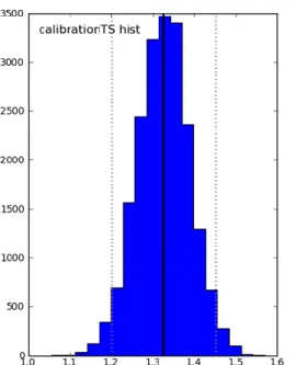
On Tore Supra, the Thomson scattering (TS) diagnostic has large error bars in its absolute calibration. Therefore an additional “recalibration” parameter is introduced in the Bayesian analysis. The TS measurements are simply multiplied by this scalar parameter (which does not change their relative values). The prior distribution for this recalibration parameter is chosen to be uniform with wide boundaries (from zero to ten) as we have no prior information on it. A typical posterior distribution for this parameter is shown in Fig. 1.
Figure 1. Posterior distribution of the Thomson scattering recalibration parameter obtained for Tore Supra pulse 47176 at t = 8.1 s.
Table 1. Error bars for the electron density reconstruction using the Bayesian analysis
Tore Supra JET
Interferometry 5*1017 m-3 20%
Thomson scattering 20% 10%*(central_density/measurement_density)2
2.5.2 Electron temperature
Boundaries of the prior distribution for each spline parameter are based on the temperature measurements. To be prudent about the outliers we define the center of the uniform distribution for a parameter as a median of the local measurements in the corresponding grid interval and then define the boundaries of the distribution as [0.5*median; 1.5*median]. Although one shouldn’t normally use measured data to define the prior in Bayesian theory, this shortcut provided a simple way to define an adequate prior distribution, without having to use much wider boundaries to avoid restricting the solution. The drawback of using very large boundaries is a penalty on the convergence time of the sampling of the posterior distribution (see 2.6). Since we are using a uniform prior distribution, the exact choice of the prior is anyway not critical for the solution as long as its boundaries are wide enough to describe the posterior distribution without cutting it.
The error bars for electron temperature profile reconstruction are presented in the Table 2 below. All the error bars include but are not necessarily equal to the instrumental error bars. They were chosen by comparing models with different values of error bars using Bayesian methods and choosing among them the values of error bars that describe the experimental data in the best way (it is a so called model selection task in Bayesian analysis theory).
Thomson Scattering 20% + 0.1keV 20% + 0.1keV
ECE 5% + 0.05keV Not used
Table 2. Error bars for the electron temperature reconstruction using the Bayesian analysis 2.5.3 Ion temperature
For the ion temperature profile reconstruction instrumental error bars specified in the experimental database were used. They were typically of the order of 50-100 eV, representing less than 10%.
2.6 Markov chain convergence
Then using a Monte Carlo Markov chain (MCMC) algorithm (Andrieu & al., 2003) implemented in a Python module pymc (Pymc) which makes sampling from the posterior distribution according to the equation (2.4) we get the samples for all the parameters. The sampling is done with a Metropolis-Hastings algorithm. The step width is tuned during the burn-in period (which duration is equal to 20% of the total number of iterations) so that the acceptance ratio was not too low neither too high. The proposal distribution is symmetric. Convergence assessment is done primarily by looking at the sample path (Figure 2, left top plot), secondly by using Geweke diagnostic (Geweke, 1992). Autocorrelation has been assessed for every sample (Figure 2, left bottom plot) and it has been checked that it decays rapidly with the increase of the distance between the elements in the Markov chain. Finally, the length of the sample was chosen high enough (typically 50 000 samples) to allow the convergence to be reached and the MCMC error stay low. A thinning of the sampled Markov chain was done with the factor of 2. Although not efficient in terms of calculation time (the calculation time was of the order of a minute for one profile), it is important in the frame of an automated and systematic analysis to make it robust and to minimize the number of cases where the convergence would not reached due to too small sample length.
Figure 2 and 3 show sampling results for one of the coefficients in the reconstruction of electron density profile for the JET shot 77922. The upper left plot shows the trajectory of the sample (values of the parameter calculated at each iteration of the MCMC algorithm). The sampling reaches rapidly a stationary state, indicating that the Markov chain has converged. The bottom left plot shows the autocorrelation and we can see that the dependence between two values of the Markov chain vanishes quickly enough (one of the properties of Markov chains) and the right plot shows the final histogram of the sample.
Figure 2. Sample of one of the coefficients in the reconstruction of an electron density profile for the JET shot 77922: the upper left plot shows the trajectory of the retained sample (value of
the parameter calculated at each iteration of the MCMC algorithm, after thinning and without the burn-in period, as a function of the iteration). The bottom left plot shows the autocorrelation (the abscissae show the distance between the elements for which the autocorrelation function is calculated, i.e. from the thinned trace). The right plot shows the histogram of the sample. This is a case of good convergence of the Markov chains.
Figure 3. Same as figure 2, but showing the trace including the burn-in period and without thinning.
Based on the samples obtained, we can calculate statistics on any quantities of our interest (for example, peaking and line-average temperature). The statistics also gives us 95% highest probability density intervals, equivalent in our case to 95 % credible intervals, which are used in the comparison with the temperature profile predictions. Further in the paper we will discuss the model used for the prediction of electron temperature profile and current diffusion.
3. Integrated modelling tools
The novelty of the developed expert system lies in the systematic and automated comparison of plasma reconstruction results with models. In this work, heat transport models predictions are compared to experiments, via the resolution of heat transport equations within an integrated modelling code. A fast integrated modelling code, METIS (Artaud & al., 2010), has been used. The key feature of METIS is to solve the heat transport equations in a simplified way, separating the treatment of the time and radial dimensions to be faster than real time (more details are given in section 4.1). Although in principle any other integrated modelling tool could have been used, the speed and robustness of METIS are key advantages in view of automated analysis of a large amount of data.
The expert system that is discussed in this work has been implemented within the framework of the European Integrated Tokamak Modeling Task Force (ITM-TF) (Falchetto & al., 2014). The two main motivations for this choice are i) the ITM-TF data Model is tokamak-generic (Imbeaux & al., 2010), thus the methods can then be applied to any experiment ii) the link with integrated modelling tools, namely equilibrium identification codes and METIS for this particular application. Moreover, the ITM-TF framework provides also methods for accessing data from various experiments, Tore Supra and JET in this application.
4. Temperature profile reconstruction and validation of heat transport models In this section we develop automated comparison criteria between reconstruction and modelling for the detailed shape of temperature profiles. One of the simple heat transport models used in METIS, with three variations of one of its parameters, is tested against a chosen experimental dataset. This illustrates an application of the method to model validation.
4.1 Heat transport and prediction of temperature profiles in METIS
The METIS code implements a simplified treatment of the heat transport equation in order to be a faster-than-real-time transport solver (an ITER pulse is simulated in about 1 minute of CPU time). To achieve this performance, METIS treats separately the time and radial dimensions of the transport equation. The time dimension is treated by solving a simple 0D equation for the plasma thermal energy content Wth:
where τE is energy confinement time, and Ploss is the total power transported through the plasma
separatrix by diffusion or convection mechanisms.
The radial dimension is treated by solving a 1D time independent transport equation for the electron and ion temperature profiles:
(4.2)
where Qe and Qi are the sums of all the electron and ion heat source terms, including the
equipartition term Qei that is proportional to (Te-Ti); is derivative of the plasma volume
enclosed in a magnetic surface with respect to the normalised minor radius x, while is the surface average of the squared gradient of the toroidal flux coordinate. The diffusion coefficients e and i are assumed to be as follows:
if KE>0 if KE=0 if K E<0 (4.3)
where μe,i is a scalar that is prescribed to be constant. Three different values of the parameter KE
are used in this work in order to test the automated comparison with three different heat transport model assumptions. The constant κ0 is found by solving the following equation, which allows a
normalization of the temperature profiles to the thermal energy content of the experiment:
(4.4)
Where W0 is an offset related to the pressure boundary condition at the LCFS.
The electron density profile is calculated from simple scaling expressions for its edge value and peaking factor (using a model that assumes that the peaking factor is proportional to the ratio between saturation density and average density), while being constrained to follow the experimental line averaged density.
Although METIS is predicting both the electron and ion temperatures, we focus the comparison on the electron temperature since it is measured during the whole pulse while we have very few Ti measurements from charge exchange in our L-mode/ohmic data set.
4.2 Steps of the analysis The analysis was done in the following steps:
1. we first run the METIS code for the whole duration of the pulse to get predictions of electron and ion temperature profiles for three models of electron diffusion coefficient (see Formula 4.3)
2. we run an equilibrium identification code (Equinox (Blum & al., 2012) in this application) to have a description of plasma equilibrium
3. map experimental measurements on the equilibrium 4. run Bayesian analysis
5. Run comparison of predicted (step 1) and reconstructed (step 4) temperature profiles 4.3 Database for the analysis
A database of 21 Tore Supra (Table 3) and 14 JET (Table 4) shots has been selected. We chose one time slice per shot to perform the analysis in a stationary phase (i.e. plasma pressure does not evolve over several characteristic transport times). All analyzed time slices were taken in ohmic or L-mode phases of the discharge. Summary tables for the Tore Supra and JET databases are presented below.
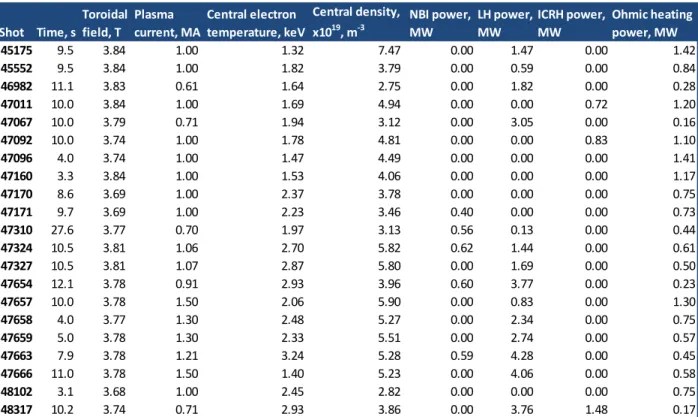
Table 3: Summary of the shots characteristics for the Tore Supra dataset: the data are taken from the METIS code, which in turn takes it from the Tore Supra database (the central density is estimated based on the peaking factor scaling laws, the central temperature is estimated based on the solution of time-independent transport equation).
Shot Time, s Toroidal field, T Plasma current, MA Central electron temperature, keV Central density, x1019, m-3 NBI power, MW LH power, MW ICRH power, MW Ohmic heating power, MW 45175 9.5 3.84 1.00 1.32 7.47 0.00 1.47 0.00 1.42 45552 9.5 3.84 1.00 1.82 3.79 0.00 0.59 0.00 0.84 46982 11.1 3.83 0.61 1.64 2.75 0.00 1.82 0.00 0.28 47011 10.0 3.84 1.00 1.69 4.94 0.00 0.00 0.72 1.20 47067 10.0 3.79 0.71 1.94 3.12 0.00 3.05 0.00 0.16 47092 10.0 3.74 1.00 1.78 4.81 0.00 0.00 0.83 1.10 47096 4.0 3.74 1.00 1.47 4.49 0.00 0.00 0.00 1.41 47160 3.3 3.84 1.00 1.53 4.06 0.00 0.00 0.00 1.17 47170 8.6 3.69 1.00 2.37 3.78 0.00 0.00 0.00 0.75 47171 9.7 3.69 1.00 2.23 3.46 0.40 0.00 0.00 0.73 47310 27.6 3.77 0.70 1.97 3.13 0.56 0.13 0.00 0.44 47324 10.5 3.81 1.06 2.70 5.82 0.62 1.44 0.00 0.61 47327 10.5 3.81 1.07 2.87 5.80 0.00 1.69 0.00 0.50 47654 12.1 3.78 0.91 2.93 3.96 0.60 3.77 0.00 0.23 47657 10.0 3.78 1.50 2.06 5.90 0.00 0.83 0.00 1.30 47658 4.0 3.77 1.30 2.48 5.27 0.00 2.34 0.00 0.75 47659 5.0 3.78 1.30 2.33 5.51 0.00 2.74 0.00 0.57 47663 7.9 3.78 1.21 3.24 5.28 0.59 4.28 0.00 0.45 47666 11.0 3.78 1.50 1.40 5.23 0.00 4.06 0.00 0.58 48102 3.1 3.68 1.00 2.45 2.82 0.00 0.00 0.00 0.75 48317 10.2 3.74 0.71 2.93 3.86 0.00 3.76 1.48 0.17
Table 4: Summary of the shots characteristics for the JET dataset: the data are taken from the METIS code (the central density is estimated based on the peaking factor scaling laws; the central temperature is estimated based on the solution of time-independent transport equation). The shots ##75225-77933 are the ones with carbon wall and the shots ##82120-84796 are the ones with ITER-like wall.
4.4 Development of automated comparison for Tore Supra and JET
Here METIS is used in a purely predictive way, we are not using any of the reconstructed profiles as input and thus we do not have prior distribution of the inputs: the result of METIS is a pointwise prediction. Therefore we are basing the comparison on checking whether this pointwise prediction lies within or very close to the 95% highest probability density (HPD) interval provided by the Bayesian analysis for various quantities that characterize the temperature profile shape. The situation would have been different if we would have reused e.g. the reconstructed electron density profile as an input to METIS. In that case it would be possible, from the probability distribution of the input, to obtain a probability distribution of the model’s response and to use acceptance criteria based on the comparison of the two distributions. Note that such an approach would have been computationally much more intensive and thus less attractive in view of a systematic application to experiments.
The comparison criteria are based on the 95% HPD intervals of various quantities that are characteristic of the accuracy of the transport model, typically the capability to predict correctly the temperature and its gradients. Although the comparison criteria have been established from a human experience of what is considered as an acceptable agreement in tokamak transport modelling, they have been “calibrated” in the sense that they have been designed on a few pulses from our dataset and then applied to the full dataset, with a verification that the resulting classification is still consistent with a human judgement of the comparison. The dataset considered here is too small anyway to apply an automated classification scheme.
Shot Time, s Toroidal field, T Plasma current, MA Central electron temperature, keV Central density, x1019, m-3 NBI power, MW Ohmic heating power, MW 75225 47.5 2.03 1.69 4.55 3.87 7.34 0.61 77895 43.0 2.69 1.47 1.05 1.88 0.00 0.92 77914 45.0 2.32 2.43 1.94 2.12 0.00 1.33 77922 45.4 2.32 2.25 1.45 2.14 0.00 1.46 77933 45.8 2.34 2.65 1.52 2.38 0.00 1.99 82120 47.9 2.20 1.97 1.39 3.62 0.00 1.61 82536 52.9 2.69 2.45 1.81 4.32 0.00 2.06 82541 52.0 2.64 2.46 1.51 5.05 0.00 4.23 84541 43.5 1.73 1.57 1.11 2.11 0.00 1.23 84543 43.5 1.73 1.57 1.10 2.08 0.00 1.21 84545 43.5 1.73 1.57 1.12 2.10 0.00 1.20 84792 43.5 1.73 1.58 1.06 2.09 0.00 1.19 84795 43.5 1.72 1.59 1.04 2.08 0.00 1.19 84796 43.5 1.72 1.58 1.11 2.08 0.00 1.17
The discrepancy estimators used for the automated comparison involve the local temperature values but also the slope of the profiles via a “gradient” and peaking factor discrepancy estimators:
relative gradient discrepancy: a ratio between minimal distance of profile gradient predicted by METIS and one of its 95% HPD boundaries (the “gradient” is calculated as T(0.3) – T (0.7) / rho(0.3) – rho(0.7) between =0.3 and =0.7)
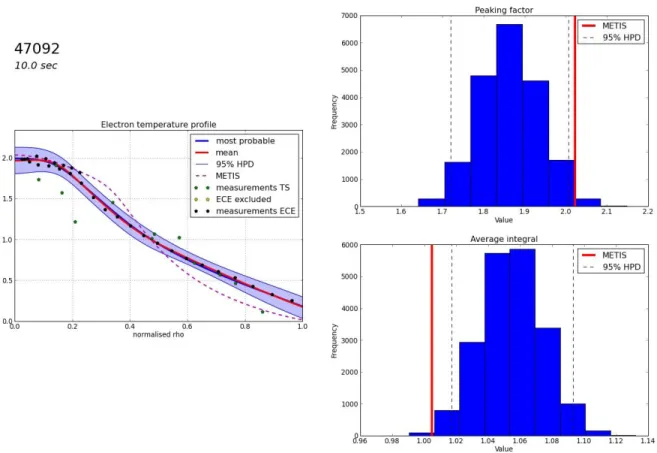
relative peaking discrepancy: a ratio between minimal distance of predicted peaking factor (a ratio between central temperature and the average one) and one of its 95% HPD boundaries
relative integral discrepancy: a ratio between minimal distance of METIS line-average integral and one of its 95% HPD boundaries
relative squared profile discrepancy on the interval [0; 0.8] for the normalized flux coordinate : a sum of squares of ratios between predicted profile and the closest boundary of 95% HPD interval (0 if the predicted profile is within the HPD interval boundaries)
These discrepancy estimators are equal to zero when the related quantity predicted by METIS is within the 95 % boundaries of the reconstructed experimental profile. A small tolerance has been added in the “comparison acceptance” criteria from the consideration of a few Tore Supra cases which were marginally outside of the 95 % HPD and would have been accepted in a “by the eyes” comparison.
In addition to these comparison discrepancy estimators, the quality of the experimental profile reconstruction is judged from the width of the 95 % HPD interval for gradient of the reconstructed profile: a ratio between upper and lower bound of the 95% HPD for gradient. If it is too high, it may point to troubles in the experimental data.
The exact value of the criteria used to consider the agreement as acceptable (see Table 5) have been derived from a few pulses from the Tore Supra database only. Then they have been applied as such to the full dataset (including JET pulses). They also provided a satisfying classification of the various pulses for the JET case, which emphasizes the tokamak-generic character of the analysis.
Quantity Value
relative gradient discrepancy 3% relative peaking discrepancy 2% relative integral discrepancy 8% relative squared profile discrepancy on the
interval [0; 0.8] 0.06
width of the HPD interval for gradient 3
Table 5: Summary of the analysis criteria to classify the agreement as “acceptable”
Examples of acceptable and not acceptable quality agreement are shown correspondingly on Figures 4 and 5. Figure 4 illustrates a case where the predicted electron temperature profile lies on almost all radial points within 95% highest probability range or is very close to it and
therefore the analysis concludes that the predictions and experimental data are in agreement. Conversely, on Figure 5 is shown an example of not acceptable agreement. The predicted electron temperature profile is visibly significantly outside of the 95 % HPD range and the profile slope is also strongly outside its 95 % HPD range.
Figure 4: Example of acceptable agreement: electron temperature profile for the shot 47171. Left plot shows the mean (read) profiles and 95% HPD interval (blue area) obtained by Bayesian analysis and METIS result (dashed magenta line); right plots show distribution for the peaking factor and average integral, their 95% HPD interval (range between dashed lines) and the METIS values (red lines).
Figure 5: Example of not acceptable agreement: electron temperature profile for the shot 47092. Left plot shows the mean (read) profiles and 95% HPD interval (blue area) obtained by Bayesian analysis and METIS result (dashed magenta line); right plots show distribution for the peaking factor and average integral, their 95% HPD interval (range between dashed lines) and the METIS values (red lines).
4.5 Application of the method for model validation
Using the criteria derived in the previous part, we applied the analysis for the diffusion coefficient model validation. We used three models as per Formula 4.3 with KE equals to 3, 0,
and -1.5. The results of our analysis are presented in the Tables 6 and 7 for Tore Supra and JET correspondingly.
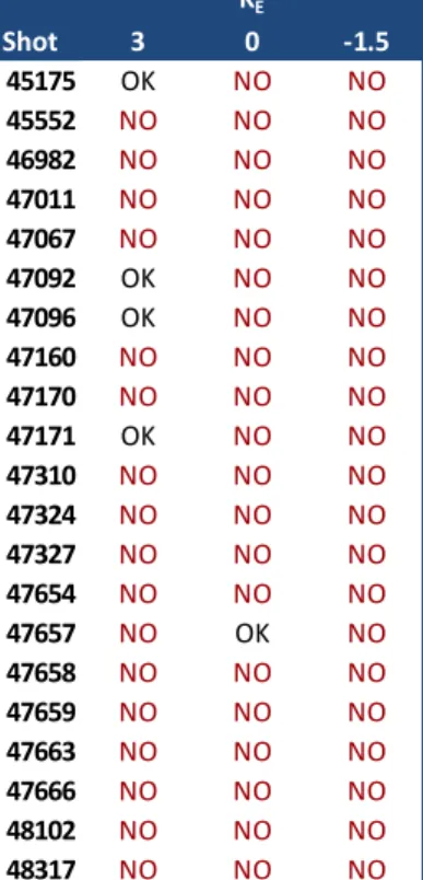
Table 6: Results of the automated comparison for Tore Supra database with three METIS runs: with KE equals to 3, 0, and -1.5. “OK” means that the agreement is acceptable, “NO”
corresponds to not acceptable agreement.
Table 7: Results of the automated comparison for JET database with three METIS runs: with KE
equals to 3, 0, and -1.5. “OK” means that the agreement is acceptable, “NO” corresponds to not acceptable agreement.
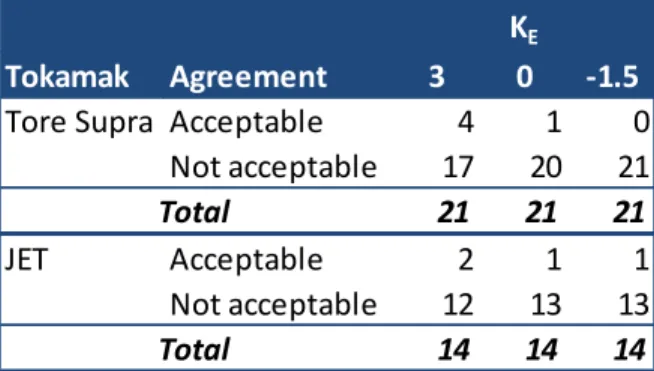
A summary on the results of our analysis is presented in the Table 8. We may see that all three models for diffusion coefficient as per Formula 4.3 with KE equals to 3, 0, and -1.5 give not
acceptable agreement in most of cases.
Shot 3 0 -1.5 45175 OK NO NO 45552 NO NO NO 46982 NO NO NO 47011 NO NO NO 47067 NO NO NO 47092 OK NO NO 47096 OK NO NO 47160 NO NO NO 47170 NO NO NO 47171 OK NO NO 47310 NO NO NO 47324 NO NO NO 47327 NO NO NO 47654 NO NO NO 47657 NO OK NO 47658 NO NO NO 47659 NO NO NO 47663 NO NO NO 47666 NO NO NO 48102 NO NO NO 48317 NO NO NO KE Shot 3 0 -1.5 75225 NO NO NO 77895 NO NO NO 77914 NO NO NO 77922 NO NO NO 77933 NO NO NO 82120 NO NO NO 82536 NO NO NO 82541 OK NO OK 84541 OK OK NO 84543 NO NO NO 84545 NO NO NO 84792 NO NO NO 84795 NO NO NO 84796 NO NO NO KE
Table 8: Summary table on results of the automated comparison for Tore Supra and JET databases with three METIS runs: with KE equals to 3, 0, and -1.5.
The conclusion of this analysis is the following: first no pulse/time slice has been rejected from too large width of the gradient HPD interval, which indicates that all experimental temperature profile reconstructions could be done in a successful way. Second, all three options tested for the transport model poorly fail to adequately reproduce the experimental profiles in most cases, although the first option (KE = 3, i.e. as per Formula (4.3)), has slightly
better statistics than the others (20 % of successful cases on the Tore Supra dataset, 14 % on the JET data set). This is not surprising, since the heat transport models used in METIS are rather simplistic while our comparison criteria were rather demanding in terms of agreement quality on the value and shape of the temperature profiles. While such simplified, scaling-based models are usually sufficient for fast scenario simulation (the main purpose of the METIS code), more sophisticated and first-principles based models are necessary for a detailed prediction of the temperature profile shape. Although it would require a longer computation time, it would be possible to apply the same automated comparison method and criteria replacing METIS with a classical Integrated Modelling suite such as CRONOS (Artaud & al., 2010) enabling solving rigorously the heat transport equations with advanced heat transport models.
4.6 Data consistency check of multi-profiles reconstruction with the energy content
The Bayesian reconstruction of the Te, Ti and Ne profiles already allowed for consistency checks for each profile. An interesting further check is to verify their overall consistency at a global level, namely by checking the plasma energy content. From these profiles and assumptions on the ion species densities, one can reconstruct with Bayesian statistics the thermal energy content
(4.5)
where is the normalized toroidal coordinate, V is the volume enclosed within the surface of coordinate , ne, Te, ni, Ti are electron density, electron temperature, ion density and ion
temperature profiles respectively.
The ion densities are calculated by METIS assuming the proportionality to the electron densities profiles, the coefficient of proportionality is calculated from the condition of electroneutrality which takes into account the effective charge (experimental one for the Tore Supra shots and the one calculated using the scaling law from (Cordey, 1985)), composition of the plasma (Deuterium in all cases) and the impurity accumulation (calculated using neoclassical simplified
Tokamak Agreement 3 0 -1.5
Tore Supra Acceptable 4 1 0
Not acceptable 17 20 21 21 21 21 JET Acceptable 2 1 1 Not acceptable 12 13 13 14 14 14 KE Total Total
formula depending on density peaking and temperature peaking from (Helander & Sigmar, 2002)).
The thermal energy is not measured directly but can be compared to the diamagnetic energy content measurement, provided an assumption (or a modelling) of the fast particle contribution to the diamagnetic energy. This can again be estimated by METIS (or any other integrated modelling code). The comparison can be used or interpreted in two ways, either as a data consistency check if the models have been validated for the conditions of the pulse or as a model validation check.
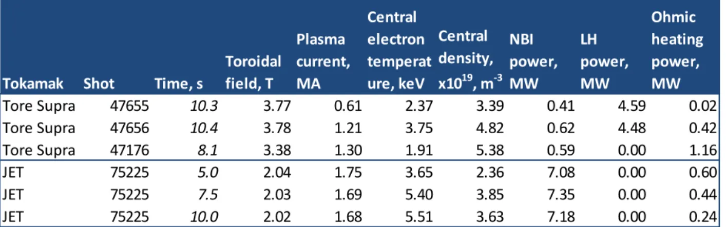
The dataset of Tore Supra and JET shots used for the calculation of the diamagnetic energy content is presented below (table 9).
Table 9: Summary of the shots characteristics for the dataset for the calculation of the diamagnetic energy content: the data are taken from the METIS code (the central density is
estimated based on the peaking factor scaling laws, the central temperature is estimated based on the solution of time-independent transport equation). The JET shot #75225 is one with carbon wall.
To calculate the probability distribution of the thermal energy we used the statistics obtained in the profile reconstruction part for all the coefficients of electron density, electron and ion temperature profiles. We then approximated the statistics of every coefficient with the continuous distribution functions using kernel density estimation technique. Using the Metropolis-Hastings algorithm we sampled from the continuous distribution functions to obtain the probability distribution for thermal energy. We calculated 95% highest probability ranges and compared them to the measured diamagnetic energy content minus the modelled fast particle energy. The quality of the agreement is determined. When this quantity is within the Bayesian range or when the discrepancy with respect to its closest bound does not exceed the uncertainty of the diamagnetic energy (typically 10 %), the quality of the agreement is judged to be acceptable. If the discrepancy is between 10 and 20 %, the agreement is judged marginally acceptable, while it is “not acceptable” if the discrepancy exceeds 20 %.
This procedure has been applied to selected time slices from four Tore Supra shots and three time slices of a JET shot. The results of the comparison are presented in the Table 10.
Tokamak Shot Time, s
Toroidal field, T Plasma current, MA Central electron temperat ure, keV Central density, x1019, m-3 NBI power, MW LH power, MW Ohmic heating power, MW Tore Supra 47655 10.3 3.77 0.61 2.37 3.39 0.41 4.59 0.02 Tore Supra 47656 10.4 3.78 1.21 3.75 4.82 0.62 4.48 0.42 Tore Supra 47176 8.1 3.38 1.30 1.91 5.38 0.59 0.00 1.16 JET 75225 5.0 2.04 1.75 3.65 2.36 7.08 0.00 0.60 JET 75225 7.5 2.03 1.69 5.40 3.85 7.35 0.00 0.44 JET 75225 10.0 2.02 1.68 5.51 3.63 7.18 0.00 0.24
Table 10: Summary table on results of the quantification of uncertainty on energy content. The columns G and H indicate the 95% highest probability range for Wth obtained by sampling from the reconstructed profiles. The column F presents the values of the thermal energy as difference between the measured diamagnetic energy (from local tokamak database) and fast particles energy calculated by the NEMO (Schneider & al, Simulation of the neutral beam deposition
within integrated tokamak modelling frameworks, 2011) and the SPOT (Schneider & al., On alpha particle effects in tokamaks with a current hole, 2005) codes. The last column contains the
discrepancy between the closest bound of the HPD range (columns G and H) and the column F (if the values from the column F are outside the range).
The six analyzed time slices indicate a good agreement, thus confirming the consistency of the profile reconstructions.
5. Quantification of uncertainty on current diffusion
Simulations of current diffusion using prescribed temperature and density profiles obtained from experimental measurements is the basic kind of analysis carried out for a tokamak pulse. It allows in particular obtaining details of the current profile that are not always measured with enough details in some experiments. Current diffusion results strongly depend, among other parameters, on the electron temperature profile through the neoclassical resistivity. Therefore uncertainties in the electron temperature profile reconstruction (which is fed as an input to such “interpretive” simulations) have a large impact on the results of the current diffusion. In this paragraph, we present an application of our automated analysis ideas to the quantification of the uncertainties on current diffusion.
5.1 Steps of the analysis
To validate current diffusion models we continued our analysis in the following way (for a given plasma discharge):
1. We reconstruct the electron temperature and density profiles from Bayesian analysis for multiple time slices of the discharge, covering its full duration with a time slice every 0.1 s. Time slices are analyzed independently and no attempt is made to correlate measurements in time.
2. we made three METIS simulations of the whole plasma discharge using the following types of electron temperature profiles: the mean profiles, the upper bound of 95% highest probability density interval profiles (i.e. “the highest possible profiles”), and the lower
from to Quality
A B C D E F=D-E G H F vs. closest G or H of agreement
Tore Supra 47655 10.3 260.0 0.0 260.0 261.8 293.1 1% OK Tore Supra 47656 10.4 472.4 0.0 472.4 459.0 522.7 0% OK Tore Supra 47176 8.1 336.7 0.0 336.7 296.9 345.9 0% OK JET 75225 5.0 2309.7 1420.0 889.7 895.6 1037.0 1% OK JET 75225 7.5 4687.1 1450.0 3237.1 2984.9 3565.3 0% OK JET 75225 10.0 4851.8 1460.0 3391.8 3286.5 4056.3 0% OK Wth (Wdia-Wfast), kJ Wth (bayesian range), kJ Discrepancy, % Tokamak Shot Time slice, s Wdia (local database), kJ Wfast (NEMO and SPOT codes), kJ
bound of 95% highest probability density interval profiles (i.e. “the lowest possible profiles”) For all the simulations we use the mean electron density profiles. At every time slice, the simulation with the highest temperature will also have the lowest flux consumption (lowest resistivity and highest non-inductive current drive efficiencies) and the slowest current diffusion, therefore representing the lowest/slowest possible result given the uncertainty on the electron temperature profile.
3. we made a comparison of the poloidal flux consumption trends and MHD activity markers obtained from three runs with the experimental one. Here the comparison is made on the appearance time of sawteeth on the ECE diagnostic and the occurrence time of the q = 1 surface in the simulation.
5.2 Prediction of current diffusion
The current diffusion model in METIS is the same as was implemented in CRONOS 1.5D code (Artaud & al., 2010) (Hinton & al., 1976). It solves the following equation for the poloidal flux
on a uniform normalized toroidal flux coordinate norm grid (which consists of 21 nodes from
norm = 0 (magnetic axis) to norm = 1 (last closed flux surface) and does not depend on time):
(5.1) where
is a time derivative of the poloidal flux at a given radial position ,
denotes the parallel conductivity (calculated according to the Sauter model (Sauter & al., 1999)),
F is the diamagnetic function, jni is the current density driven by the non-inductive sources, R is the major radius, 0 is the magnetic permeability of free space, the value of the un-normalised toroidal flux coordinate at the last closed flux surface, B0 the value of the toroidal magnetic field involved in the definition of the toroidal flux coordinate and the normalised toroidal flux coordinate
m norm
. The notation indicates a magnetic flux surface average, defined as the volume average of a quantity around a flux surface of radial coordinate , i.e. in an elementary volume dV enclosed between two magnetic surfaces distant of d
The line-average effective charge measurement from bremsstrahlung is used to prescribe the effective charge, assuming a flat profile.
Non-inductive current drive external sources (NBI for the JET shot, LHCD for the Tore Supra one) are calculated self-consistently by the models included in METIS. The model for LHCD efficiency is the empirical model described in (Goniche & al, 2005).
METIS also implements a sawtooth model that accounts for the time-averaged effects of sawteeth. Applied here to the current diffusion, it prevents the q-profile from going below 1 by clamping it to the q = 1 surface.
5.3 Results
First we analyse Tore Supra pulse #47658, an L-mode pulse featuring two plateaus of LHCD power, (~4.5 MW from t = 5 to 10 s, then ~3.3 MW from t = 10 to 12 s, see fig. 6).
Figure 6: Overview of the Tore Supra shot #47658. The upper plot shows plasma current and its components throughout the length of the shot. The middle plot shows the heating scheme. The bottom plot shows other important parameters like loop voltage, li, p
A first global analysis of the flux consumption is shown on the Figure 7. The flux consumption of the simulation using the mean temperature profiles are in excellent agreement with the experimental measurement, which provides a simultaneous validation of the current diffusion model used (including the LH current drive efficiency) and the reconstructed Te profiles during the various phases of the pulse. The two other simulations with highest and lowest profiles in the 95% HPD interval introduce a confidence interval around the simulation with mean profiles. Nonetheless such a global view is integrating the instantaneous flux consumption over the whole pulse. There can be cases where the flux consumption is overestimated during a particular phase of the pulse, then this overestimation is later on compensated by an underestimation of the flux consumption in another phase, always staying within the confidence interval. Therefore the global analysis should be supplemented by an instantaneous analysis of whether the modelled flux consumption is consistent with the confidence interval of the electron temperature at a given time slice. To do this, we have calculated the time derivative of the consumed flux and smoothed it using Savitzky-Golay filtering procedure implemented in MATLAB (MathWorks, 2014), with polynom order = 2 and a window with is equal to 51 points for the JET pulse and 5 for the Tore
Supra shot (the difference comes from the fact that the JET METIS run has a higher time resolution than the Tore Supra one). The results are presented on Figure 8.
Figure 7: Consumed poloidal flux comparison for the Tore Supra shot #47658. The blue lines shows the results of the METIS run with HPD interval profiles as an input; the red line is the result of the METIS run with the mean profiles as an input. The greed line is the experimental measurements. Note that the offset poloidal flux consumption is unknown thus it was determined as the difference between the mean METIS run and experimental trend in the beginning of the shot.
Figure 8: Comparison of filtered time derivatives of the consumed poloidal flux for the Tore Supra shot #47658. The blue lines shows the results of the METIS run with HPD interval profiles
as an input; the red line is the result of the METIS run with the mean profiles as an input. The green line is the experimental measurements.
To develop an automated method for the comparison of derivatives of consumed flux we calculated the discrepancy between i) the experimental values and the closest boundary of the highest probability density range and ii) the experimental values and the mean temperature simulation. The discrepancy then was normalized to the maximum loop voltage that would be obtained in a steady state where the current would be fully inductively driven, which is equal to the plasma current times plasma resistivity (estimated using the mean electron temperature). The results are presented on the Figure 9. The first discrepancy estimator is zero when the flux time derivative within the confidence interval and therefore allows determining whether the experimental flux consumption is within or outside the Te errorbars. The second one allows the relevance of a single simulation, done with the mean Te. The normalized discrepancy is chosen instead of the relative discrepancy, for two reasons. First, in phases with large non-inductive current drive, the flux consumption tends towards zero, making the relative discrepancy very large. Moreover, in such a case, the discrepancy would be due essentially to the non-inductive current models, for which the temperature dependence is weaker than for the resistive flux consumption in ohmic phases, i.e. the discrepancy has less probability to arise from the electron temperature uncertainties.
A threshold of +/- 0.3 is chosen to define an acceptable agreement in the automated comparison process. This value is chosen so that the system would detect the flux consumption deviation between the experiment and the simulation with mean Te occurring around t = 12 s on this Tore Supra case. Indeed, a human judgment of figure 7 would conclude that this is the only time where a significant deviation is observed. The idea is that the comparison criterion value provides the same conclusion, in a quantified way so that it can be automatized.
Figure 9: Normalized discrepancy between experimental values for the consumed flux
derivative and the closest boundary of the highest probability density range simulations (in blue) and the normalized discrepancy between experimental values and the mean simulation (in red) for the Tore Supra shot #47658. The cyan lines show the boundaries of acceptable agreement (+/- 0.3).
For the Tore Supra case, the discrepancy with the confidence interval (red curve on Figure 9) is almost always within the acceptability threshold, indicating that the experimental flux consumption is consistent with the electron temperature uncertainties. It does not imply that the Te uncertainties are necessarily the cause of the discrepancy between experiment and the mean Te simulation, but they could potentially explain it.
When the discrepancy with the confidence interval is within the acceptability threshold, one can use the two HPD simulations to determine the confidence interval on the safety factor profile. This is illustrated for the Tore Supra case at t = 2 s in figure 10.
Figure 10: q-profiles at t = 2 s for the Tore Supra shot #47658. The red line corresponds to the METIS simulation with the mean Te profiles. The two blue lines correspond to the METIS simulations with the highest and lowest possible Te profiles
We can also verify that MHD markers dynamics, e.g. the time of appearance of sawteeth, are consistent with the confidence interval (table 11).
Table 11: Summary table on results of the comparison of sawteeth onset time for the Tore Supra shot #47658. The second column indicates what type of temperature profiles are used as
an input to the METIS code. The experimental sawteeth onset time is determined from ECE Shot Te profiles used in METIS Sawteeth onset time, s TS@47658 HPD up 3.4 mean 2.3 HPD low 1.8 Experiment 1.9
measurements, while in METIS it is determined by the onset of the q-profile clamping to the q = 1 surface.
We now apply the same analysis to the carbon wall JET shot #75225 (hybrid scenario). An overview of its scenario is shown on the Figure 11. A high level of NBI power is injected just after a plasma current overshoot in order to optimize the current profile and freeze it as long as possible during the H-mode phase (from t ~ 45 s to 50.5 s). The flux consumption in this phase is close to 0, owing to almost fully non-inductive current drive. It is even negative (transformer recharge) during the reduction of the plasma current after the overshoot.
Figure 11: Overview of the JET shot #75525. The upper plot shows plasma current and its components throughout the length of the shot. The middle plot shows the heating scheme. The bottom plot shows other important parameters like loop voltage, li, p
Applying the same procedure as in the Tore Supra case, a set of three simulations is carried out using the recommended Zeff processing that can be found in the JET database, namely the values in PPF/KS3/ZEFV, corresponding to a vertical line of sight of bremsstrahlung measurement. The results are indicated on the Figures 12-14 (the consumed flux, the time derivative, and the absolute discrepancy).
Figure 12: Consumed poloidal flux comparison for the JET shot #75225. The red line corresponds to the METIS simulation with the mean Te profiles. The two blue lines correspond to the METIS simulations with the highest and lowest possible Te profiles. The green line is the experimental flux consumption. Offset calculated at the initial time of the simulation and profile reconstruction
Figure 13: Comparison of filtered derivatives of consumed poloidal flux for the JET shot #75225. The blue lines shows the results of the METIS run with HPD interval profiles as an
input; the red line is the result of the METIS run with the mean profiles as an input. The green line is the experimental measurements
Figure 14: Normalized discrepancy between experimental values for the consumed flux derivative and the closest boundary of the highest probability density range simulations (in blue) and the relative discrepancy between experimental values and the mean simulation (in red) for the JET shot #75225. The cyan lines show the boundaries of acceptable agreement (+/- 0.3). In this case, the discrepancy between the experimental values and the HPD range simulations (the blue line on the Figure 14) stays within the acceptable threshold throughout the whole pulse except for the transitional phases where the neutral beam injection was switched on and off (around t = 5 s and t = 11 s) and a few time slices in between where the discrepancy is explainable by the noise in the effective charge measurements.
Figure 15 illustrates the confidence interval on the q-profiles obtained at t = 7.0 s. Table 12 shows the comparison with the sawteeth onset time, which appear in the experiment at a time consistent with the determined errorbars of the simulation.
Figure 15: q-profiles at t = 7.0 s for the JET shot #75225. The red line corresponds to the METIS simulation with the mean Te profiles. The two blue lines correspond to the METIS simulations with the highest and lowest possible Te profiles.
Table 12: Summary table on results of the comparison of sawteeth onset time for the JET shot #75225. The second column indicates what type of temperature profiles are used as an input to the METIS code. The experimental sawteeth onset time is determined from HRTS measurements, while in METIS it is determined by the onset of the q-profile clamping to the q = 1 surface. 6. Conclusion Shot Te profiles used in METIS Sawteeth onset time, s JET@75225 HPD up 8.0 mean 5.4 HPD low 4.6 Experiment 5.2
The present work was devoted to the development of an automated comparison method between Bayesian reconstruction of plasma profiles and time dependent solutions of the transport equations. Two major applications have been shown: the former is aimed at comparing electron and ion temperature profiles to heat transport modelling. This quite classical type of analysis has been fully automated and the highest probability density intervals coming from the Bayesian reconstruction have been used to define various comparison criteria on the temperature profile shape (average gradient, peaking factor,..). This method can be applied to model validation of a simple heat transport model with three radial shape options. It has been tested on a database of 21 Tore Supra and 14 JET shots. All three choices of the radial shape parameter have been found not to meet the “acceptable agreement” criteria, indicating that more sophisticated, physics based transport models should be used for such detailed comparison of the temperature profile shape. Another application of the multi-profile reconstruction which has been carried out (ne, Te and Ti) is a data consistency check on the plasma energy content.
The second application aims at quantifying uncertainties due to the electron temperature profile in current diffusion simulations. A systematic reconstruction of the Te profiles is first carried out for all time slices of the pulse. The Bayesian 95% highest probability density intervals on the Te profile reconstruction are then used for i) data consistency check of the flux consumption and ii) defining a confidence interval for the current profile simulation. The latter can be further used to compare with possible MHD markers such as the onset time of sawteeth. The method has been applied to one Tore Supra pulse and one JET pulse.
The implementation of both applications is tokamak-generic as was performed using the ITM-TF framework. The proposed method therefore provides a combination of automated comparison between simulation and experiment, data consistency checks and uncertainty quantification in simulations, all based on the highest probability density intervals arising from Bayesian profile reconstruction.
Although Bayesian analysis is an attractive and rigorous method to calculate error bars, it is not employed in a routine way in most present fusion experiments. Our hope is that our work will help to spread its usage. The idea of a unique integrated modelling platform for deploying both plasma reconstruction and predictive tools provides the opportunity of using a whole range of predictive models and even to integrate some of them directly in the reconstruction if some measurements are missing. It also allows a variety of high order data consistency checks, such as the diamagnetic energy content which involves three profile reconstructions and assumptions on the impurity and fast particles content, and the verification of the consistency of the flux consumption. Our work provides a prototype implementation of this idea, resulting in a tokamak generic and automated tool to deal with the massive amount of data to be produced by long pulse plasma experiments.
Acknowledgements
The authors would like to thank Dr. Rainer Fischer for his support and fruitful discussions on the implementation of Bayesian analysis.
This work has been carried out within the framework of the EUROfusion Consortium and has received funding from the European Union’s Horizon 2020 research and innovation programme under grant agreement number 633053. The views and opinions expressed herein do not
References
Andrieu, C., & al. (2003). An introduction to MCMC for machine learning. Machine Learning,
50, 5-43.
Artaud, J., & al. (2010). The CRONOS suite of codes for integrated tokamak modelling. Nuclear
Fusion, 50, 043001.
Berger, J. (1985). Statistical Decision Theory and Bayesian Analysis. Springer.
Beurskens, M., & al. (2011). H-mode pedestal scaling in DIII-D, ASDEX Upgrade, and JET.
Physics of Plasmas 18, 056120.
Blum, J., & al. (2012). Reconstruction of the equilibrium of the plasma in a Tokamak and
identification of the current density profile in real time. Journal of computational physics
231, 960.
Cordey, J. (1985). Unification of Ohmic and Additionally Heated Energy Confinement Scaling
Laws, JET-P(85)28. Varenna, Italy.
Dinklage A., a. (2012). Integrated diagnostics design. Fus. Sci. Technol., 62, 419. Falchetto, G., & al. (2014). The European Integrated Tokamak Modelling (ITM) effort:
achievements and first physics results. Nuclear Fusion, 54, 043018. Fischer, R. (2010). Fus. Sci. Technol., 58, 675.
Fischer, R., & al. (2006). Flexible and reliable profile estimation using exponential splines.
Bayesian Inference and Maximum Entropy Methods in Science and Engineering, AIP conference proceedings 872, 296-303.
Geweke, J. (1992). Evaluating the accuracy of sampling-based approaches to calculating
posterior moments. In Bernardo et al,: see also
http://pymc-devs.github.io/pymc/modelchecking.html#convergence-diagnostics.
Gil, C., & al. (2009). Diagnostic systems on Tore Supra. Fusion Science and Technology, 56, 1219.
Goniche, M., & al. (2005). Lower Hybrid current drive efficiency on Tore Supra and JET.
Sixteenth Topical Conference on Radio Frequency Power in Plasmas.
Helander, P., & Sigmar, D. (2002). Collisional transport in magnetized plasma, p.93. Cambridge university press.
Hinton, F., & al. (1976). Theory of plasma transport in toroidal confinement systems. Reviews of
modern physics, 48, 239-308.
Imbeaux, F., & al. (2010). A generic data structure for integrated modelling of tokamak physics and subsystems. Computer Physics Communications 181, 987-998.
Lister J.B., a. (2003). The ITER project and its data handling requirements. Proceedings of
ICALEPS 2003, (p. 589). Gyeongju, Korea.
MathWorks. (2014). Retrieved from MathWorks:
http://www.mathworks.fr/fr/help/signal/ref/sgolayfilt.html
Pymc. (n.d.). Retrieved from http://pymc-devs.github.io/pymc/index.html
Sauter, O., & al. (1999). Neoclassical conductivity and bootstrap current formulas for general axisymmetric equilibria and arbitrary collisionality regime. Physics of plasmas, 6, 2834-. Schneider, M., & al. (2011). Simulation of the neutral beam deposition within integrated
tokamak modelling frameworks. Nuclear Fusion, 51 , 063019 (15pp).
Schneider, M., & al. (2005). On alpha particle effects in tokamaks with a current hole. Plasma
van Milligen, B., & al. (2011). Integrated data analysis at TJ-II: The density profile . Review of
scientific instruments 82, 073503.
Verdoolaege G., a. (2010). IEEE Trans. Plasma Sci., 38, 3168. von Toussaint, U. (2011). Rev. Mod. Phys., 83, 943.