A 2D and 3D thermal model of powder injection laser cladding

a

Corresponding author: ra.tjardin@ulg.ac.be

A 2D and 3D thermal model of powder injection laser cladding

Rúben António Tomé Jardin1, a, Hoang Son Tran1, Neda Hashemi2, Jacqueline Lecomte-Beckers², Raoul Carrus³ and Anne Marie Habraken1

1

University of Liège, ArGEnCo (Architecture, Geology, Environment and Construction) Department, MS2F (Structures, Fluids and Solid Mechanics) Unit, Liège, Belgium

2

University of Liège, A&M (Aerospace and Mechanical Engineering) Department, MMS (Metallic Materials Science) Unit, Liège, Belgium;

³SIRRIS, Liège, Belgium.

Abstract. Thermal 2D and 3D finite element models were elaborated to retrieve the high temperature gradients

generated during multi-layer laser cladding deposition. The model can deliver the complete thermal history of the deposition process. Convection and radiation phenomena were taken into account. Key points from the specimen had their temperature evolution saved with thermocouples during the production and used later to calibrate the numerical model. The method to compute the heat input in the 2D model once the 3D model has been validated is described. An accurate thermal history of the specimens is the first step to predict crack by thermo-mechanical model and microstructure by thermo-metallurgical model.

1 Introduction

Laser cladding is an additive manufacturing process that uses a laser as heat source. This process is able to manufacture a large variety of alloys. These characteristics make laser cladding a promising technology for repairing and coating existing pieces but also for near net to shape manufacturing. Nevertheless this process is not yet mastered. Crack formation, bad quality deposits and geometrical distortions are still a reality in this process. To provide a better understanding of the phenomena, process simulations are proposed as a way towards optimal solutions.

1.1 Numerical models

Kim et al. [1] studied the dilution and melt pool shape in laser cladding with wire feeding using a 2D finite element thermal model with adaptive mesh (Figure 1). Some simplifications were made, like not considering conductivity, specific heat and density as temperature dependent properties. Also latent heat and convection within the melt pool were neglected.

Figure 1 - Adaptative mesh (dashed lines identify isovalues of

temperature) [1]

To generate the adaptive mesh, the authors start by assuming the geometry of deposit due to powder and substrate melting by the laser power. After the simulation of the first track, a new melting line is further defined. By

comparing the original line and the new one, the mesh is adapted to the new one. This iterative process is continuously repeated until the difference between the previous line and the new one is under a certain defined tolerance. Regarding the dilution (between the alloys of the deposit and the substrate) they concluded that the dilution increases with cladding time. Also the melting rate is faster in the beginning and reduces after a few seconds. With the increase of laser power the dilution increases. The changes in depth and width of the melt pool have the same tendency as the dilution, to increase with laser power. However the changing rate in depth is slower than in the width. With the increase of substrate preheating, the dilution increases. During the cladding process the width of the melt pool within the substrate changes faster than the melt pool of the clad. Finally, one way to maintain low dilution is to decrease the laser power so that the melt pool stays small and consequently the dilution is also maintained small.

Labudovic et al. [2] developed a 3D thermo mechanical decoupled model to study the size of the melt pool and to compute the residual stress in a thin wall of ten layers. The materials are AISI 1006 as substrate and Monel 400 alloy as clad material. They used an on-line high-shutter speed camera to retrieve data from the melt pool and after the cladding microstructural and x-ray analysis were conducted. The dimensions of the melt pool were correlated with the thermal conditions at solidification. The results from the heat transfer analysis were used as input in the mechanical finite element model to obtain the stress state. The residual stresses from the experiments were investigated using the x-ray diffraction technique and the results were correlated with the numerical ones. For the experimental part, the laser power varied between 300 and 1000 W and the speed of the laser varied between 5 and 15 m/s. Comparing the size and shape of the melt pool for different laser powers and velocities they found a good agreement between simulations and experiments. They concluded that an

MATEC Web of Conferences

increase of the laser power and a decrease of the laser speed result in a wider melt pool.

The work presented hereafter is the first step of a study focused on shape prediction for the cladding of a high speed steel alloy. In a similar way to Labudovic et al. [2] the thermal model is the basis of the mechanical approach. Therefore it was chosen to carefully validate the 2D thermal model by experiment. As in Kim et al. [1] successive manual mesh refinements are ongoing to get an accurate temperature distribution. However the first problem to face is the difference between the 3D experiment where 4 thermocouples are available and the 2D thermal model which neglects the fact that thermal flow happens in the third direction. The current paper presents the numerical adjustment of 2D laser heat input compared to the 3D heat input to get a similar temperature distribution. The research focusses on a large deposit of 20 mm x 20 mm with 13 tracks and 25 layers. So a thermomechanical 3D model of the total process is too expensive from the CPU point of view and in addition the thermocouple measurements and the microstructure identification confirm that middle track can be representative. These considerations explain why the focus here is preliminary to identify the link between 3D and 2D thermal models.

1.2 Finite element software used

The thermo-mechanical-metallurgical finite element software used is Lagamine [3]. This software is in development by the University of Liège since 1985. It has already been applied on the modelling of different processes like thermomechanical processes of continuous casting [4], manufacturing of bimetallic rolling mill rolls [5] and incremental sheet forming process [6-7]. This code has a switch on switch off element capacity allowing to model the material deposition.

2 Modelling

2.1.1 2D mesh

To find the optimal mesh, an initial mesh convergence study was carried on with the goal to compute a thermal gradient distribution predicting the melting line in a stable way. The optimal mesh is refined enough to deliver accurate results in the zone of interest while at the same time coarse enough to provide fast simulations. The selected mesh (Figure 2Figure 2) is the one called 54 (Figure 3), meaning it has 54 element to model one track. This mesh has an element size of 0.74 mm in the deposit zone, which corresponds to half of the diameter of the modelled laser beam.

2.1.2 3D mesh

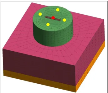
The 3D mesh was created with the same size of element in the most refined area (Figure 4) as in the 2D mesh. It has nodal points at the location of the 4 thermocouples that are located 5 mm under the substrate surface, at a distance of 20 mm from the edge of the periphery of the substrate (see yellow dots in Figure 4).

Figure 2 - Chosen 2D mesh

Figure 3 - Temperature distribution from the 2D mesh at the edge of the deposit track in depth direction when the laser beam is in the middle of the deposit

Figure 4 - 3D mesh, the red dot models the laser flow used to calibrate 2D-3D transfer factor

2.2 Process modelling

For the construction of the thermal model two thermal laws were required. First the heat transfer by conduction and accumulation given by:

int p T T T T k k k Q c x x y y z z  t     _   _  _{ }                     (1) 195 mm 100 mm 40 mm

Where k is the thermal conductivity coefficient, T is the temperature, Qint is the heat generation/extraction, ρ is

the mass density of the material, cp is the specific heat

capacity and t is the time.

Secondly the exchange of heat by convection and radiation is given by:

4 4

0 0

.(

. )

(

)

(

)

K

T n

h T

T



T

T





 







ambient temperature, T is the surface temperature, ε is the emissivity and σ is the Stefan-Bolzmann constant.

All the material parameters (k, ρ, cp and T0 except h

and ε) were measured as described in [8]. The boundary conditions (h and ε) were taken from the literature and checked by the modelling of the substrate’s cooling for well-known temperature history defined by a preheating step.

The flux was applied on the surface of four elements with a size approximated from the one of the laser flux.

3 Results

The intensity of the heat flux input was calibrated to be consistent with experimental remelting depth.

To achieve the same melting depth in the 2D simulation (Figure 5) as in the metallurgic observations and similar temperature level as measured by the thermocouple, the value of the laser power used in the experiments had to be divided by a factor of 4.7. Simplifications, as for example, not considering a third direction for heat to dissipate oblige to decrease the power from experiment to simulation in 2D.

Figure 5 - 2D simulation

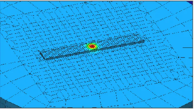
For the 3D simulation (Figure 6), the power of the laser beam is the value of the 2D simulation multiplied by 1.17. This 2D-3D factor was achieved by applying a localized flux in the 2D and 3D thermal models (see red dot in Figure 4) to get the same maximum temperature. Considering a third direction for heat to dissipate implies the need for more power in the 3D simulation.

These factors are true for the chosen combination of parameters

4 Current work and conclusion

Within this preliminary numerical study, the following topics were developed: required element size, optimal mesh, set of material data as well as the link between 2D and 3D models. The thermal model was calibrated on a large deposit where 4 thermocouples gave the thermal history. The required experiments to more accurately identify the boundary condition were based on this first step

The current work consists in better adjusting the boundary conditions corresponding to the calibration of the laser power and the values for convection and

radiation by accurate comparison between the 3D thermal model and new experimental data related to thin wall deposit and 7 thermocouples.

Figure 6 - 3D simulation

References

1. J. Do Kim and Y. Peng, “Melt pool shape and dilution of laser cladding with wire feeding,” J.

Mater. Process. Technol., vol. 104, no. 3, pp. 284–

293, (2000).

2. K. Labudovic, HU, “A three dimensional model for direct laser metal powder deposition and rapid prototyping,” vol. 8, pp. 35–49, 2003.

3. S. Cescotto, H. Grober, “Calibration and application of an elastic viscoplastic constitutive equation for steels in hot-rolling conditions”, Eng. Comput, vol. 2(2),pg.101–6 (1985).

4. F. Pascon, S. Cescotto, AM Habraken, “A 2.5 D finite element model for bending and straightening in continuous casting of steel slabs”, Int. J. Numer. Methods Engng, vol. 68, 125-149, (2006).

5. I. Neira Torres, G. Gilles, P. Flores, J. Lecomte-Beckers, A.M. Habraken “FE modelling of the cooling and tempering steps of bimetallic rolling mill rolls”, Int . J. Material Forming, (2015).

6. C. Henrard , C. Bouffioux, P. Eyckens, H. Sol, J. Duflou, P. Van Houtte, A. Van Bael, L. Duchene, A. Habraken, “Forming forces in single point incremental forming: prediction by finite element simulations, validation and sensitivity”, Engineering, computing & technology, vol. 47, pp 573-590 (2011).

7. C. Guzmán, A. Bettaieb, J. Sena, R. Alves de Sousa, A. Habraken, L. Duchene, ”Evaluation of the Enhanced Assumed Strain and Assumed Natural Strain in the SSH3D and RESS3 Solid Shell Elements for Single Point Incremental Forming Simulation”, Trans Tech Publications, vol. 504-506, pp. 913-918, (2012).

8. A. Mertens, S. Reginster, H. Paydas, Q. Contrepois, T. Dormal, O. Lemaire, J. Lecomte-Beckers, Powder Metallurgy, vol. 57 (3), pp. 184-189, (2014).