Any correspondence concerning this service should be sent
to the repository administrator:
[email protected]
This is an author’s version published in:
http://oatao.univ-toulouse.fr/24697
To cite this version: Chen, Zhouye and Basarab, Adrian and
Kouamé, Denis Semi-blind ultrasound image deconvolution from
compressed measurements. (2018) Ingénierie et Recherche
BioMédicale, 39 (1). 26-34. ISSN 1959-0318
Official URL
DOI :
https://doi.org/10.1016/j.irbm.2017.11.002
Open Archive Toulouse Archive Ouverte
OATAO is an open access repository that collects the work of Toulouse
researchers and makes it freely available over the web where possible
Semi-Blind
Ultrasound
Image
Deconvolution
from
Compressed
Measurements
Z.
Chen
a,∗,
A.
Basarab
b,
D.
Kouamé
ba InstituteofSensors,SignalsandSystems,Heriot-WattUniversity,EH144AS,UK b UniversityofToulouse,IRIT,UMRCNRS5505,Toulouse,France
Highlights
• EstimatingthePSFatthesame time in the recently proposed compressive deconvolution framework for ultrasound imaging.
• Taking fully advantage of the existingmethodofPSF estima-tion.
• Presenting an analytical solu-tiontothesub-problemofPSF.
Graphicalabstract
Abstract
Therecentlyproposedframeworkofultrasoundcompressivedeconvolutionoffersthepossibilityofdecreasingtheacquireddatawhile improv-ingtheimagespatialresolution.Bycombiningcompressivesamplingandimagedeconvolution,thedirectmodelofcompressivedeconvolution combinesrandomprojectionsand2Dconvolutionwithaspatiallyinvariantpointspreadfunction.Consideringthepointspreadfunctionknown, existingalgorithmshaveshowntheabilityofthisframeworktoreconstructenhancedultrasoundimagesfromcompressedmeasurementsby in-vertingtheforwardlinearmodel.Inthispaper,weproposeanextensionofthepreviousapproachforcompressiveblinddeconvolution,whoseaim istojointlyestimatetheultrasoundimageandthesystempointspreadfunction.Theperformanceofthemethodisevaluatedonbothsimulated and in vivoultrasounddata.
Keywords:Ultrasoundimaging;Compressivesampling;Blinddeconvolution
1. Introduction
Despite its intrinsic rapidity of acquisition, several ultra-sound (US) applications such as duplex Doppler or 3D imaging
* Correspondingauthor.
E-mailaddress:[email protected](Z. Chen).
may require higher frame rates than those provided by conven-tional acquisition schemes or may suffer from the high amount of acquired data. In this context, compressive sampling (CS) framework appears as an appealing solution to overcome these issues. Since the first works in compressive US imaging pub-lished in 2010 [1–4], there have been several studies devoted to this topic to date [5–11]. Conventional approach to sample
nals or images follows the Shannon–Nyquist theorem. Accord-ing to the Shannon–Nyquist samplAccord-ing theorem, the samplAccord-ing rate must be at least twice the maximum frequency contained by the signal. However, the theory of CS makes it possible to go against the common knowledge in data acquisition. It al-lows to recover, via non linear optimization routines, an image from few linear measurements (below the limit standardly im-posed by the Shannon–Nyquist theorem) provided two condi-tions: i) the image must be sparse in a known basis or frame and ii) the measurement matrix must be incoherent with the sparsifying basis [12]. Existing works focused on these two as-pects, i.e. the sparsity study and the incoherent acquisition, have shown that it is possible to recover US radio-frequency (RF) images based on their sparsity in basis such as 2D Fourier trans-form [13], wavelets [14], waveatoms [15], or learning dictionar-ies [6], using various acquisition schemes such as projections on Gaussian [4]or Bernoulli random vectors [13], plane-wave emissions [14]or Xampling [5].
However, despite the promising results, there are still two re-maining problems regarding the application of CS in US imag-ing. i) Since perfect sparsity is almost never reachable due to the presence of noise and the incoherence between measurement matrix and sparse basis cannot be easily satisfied in practical situations, the images reconstructed from compressed measure-ments tend to be less good compared to standard acquisitions, especially for a low number of measurements. ii) In the case where an exact CS recovery is possible, i.e., the quality in terms of resolution of the recovered US images is equivalent to those acquired using standard schemes, whereas it is widely accepted that image quality is one of the open challenges in US imag-ing. The signal-to-noise ratio, the spatial resolution and the contrast of standard US images are affected by the physical phenomenons related to US wave propagation and limited by the bandwidth of the transducer of imaging system.
Image deconvolution represents a valuable tool that can be used for improving image quality without requiring com-plicated calibrations of the real-time image acquisition and processing systems. US image deconvolution has been exten-sively studied in the literature, showing very promising results
[16–18]. Motivated by the interest of CS and deconvolution, we have recently proposed a framework called compressive de-convolution (CD) in US imaging [19]. The objective was to reconstruct enhanced RF images from compressed linear mea-surements, aiming to obtain a higher frame rate or less data volume and to enhance the image contrast at the same time. The main idea behind CD is to combine CS and deconvolution, leading to the following linear direct model:
y= 8H x + n (1)
where y ∈ RM stands for the M linear compressed
mea-surements obtained for one RF image H x and 8 ∈ RM×N (M << N ) corresponds to the CS acquisition matrix. The RF image H x models that the tissue reflectivity function (TRF) x∈ RN is degraded by H ∈ RN×N, which is a block circulant
with circulant block (BCCB) matrix related to the 2D PSF of the US system. Finally, n ∈ RM represents a zero-mean
addi-tive white Gaussian noise. We emphasize that all the images in
(1)are expressed in the standard lexicographical order. Inverting the model in (1) will allow us to estimate the TRF x, which is considered as a higher resolved US image, from the compressed RF measurements y. Though similar models have been recently proposed for general image pro-cessing purpose [20–23] including a theoretical derivation of RIP for random mask imaging [24], we formulated in [19]the reconstruction process into a constrained optimization problem exploiting the relationship between CS recovery and deconvo-lution: min x∈RN,a∈RNk a k1+αkxk p p+ 1 2µk y − 89a k 2 2 s.t. H x= 9a (2)
where a is the sparse representation of the US RF image H x in the transformed domain 9. It enables the reconstruction of the RF image and the TRF at the same time. α and µ are hy-perparameters balancing the weight of each term in the cost function to minimize. The optimization problem above includes three terms: i) the ℓ1-norm term aiming at imposing the
spar-sity of the RF image in the sparse basis 9, ii) the ℓp-norm term
modeling the a priori of the target image x, where the shape parameter p related to the Generalized Gaussian Distribution (GGD) is ranging from 1 to 2 (1 ≤ p ≤ 2), allowing us to gen-eralize the existing works in US image deconvolution mainly based on Laplacian or Gaussian statistics [25,26], iii) the data fidelity term.
In order to solve this problem, an algorithm based on the Alternative Direction Method of Multipliers (ADMM) was initially proposed in [19] and was further improved with faster convergence based on Simultaneous Direction Method of Multipliers (SDMM) in [27]. Both algorithms have achieved promising results with the assumption that the PSF was known or could be estimated in a pre-processing step. However, the PSF cannot be perfectly known in practical situations. An ini-tial investigation to jointly estimate the PSF has been recently published in [28]to show the possibility of recovering RF im-age, TRF and PSF at the same time.
In this paper, following the previous work and exploiting the prior information on the PSF, we propose and detail a compres-sive semi-blind deconvolution (CSBD) algorithm. The results on simulated and experimental images show improved perfor-mance compared to the non-blind approach. The remainder of this paper is organized as follows. In Section2we formulate the compressive semi-blind deconvolution problem. Section3 de-tails our proposed CSBD algorithm and simulation results are shown in Section4before drawing the conclusions in Section 5. 2. Methods
2.1. Problem formulation
Given the commutativity of the 2D convolution product, let us write the CD direct model in a different form, that includes the PSF kernel h instead of the associated BCCB matrix H :
y= 8XP h + n (3) where X ∈ RN×N is a Block Circulant with Circulant Block (BCCB) matrix with the same structure as H , with the circulant kernel x ∈ RN. h ∈ Rn represents the PSF with a support of size n. P ∈ RN×nis a simple structure matrix mapping the n coefficients of the PSF kernel h to a N length vector so that H x= XP h. Its definition and implementation details can be found in Appendix A.
Inspired by the existing joint identification methods for blind deconvolution problem [26,29,30] and the prior information about the PSF such as the sampling frequency of the system, we formulate the compressive semi-blind deconvolution prob-lem as below. min x∈RN,a∈RN,h∈Rsk a k1+αkxk p p+ γ k h − h0k22 + 1 2µk y − 89a k 2 2 s.t. H x= 9a (4)
where h0represents an initial guess of the PSF and γ is a
posi-tive hyper-parameter. The objecposi-tive function in (4)contains, in addition to the three terms that we detailed in the introduction, a regularization term for the PSF. Similar to [31,32], we hereby incorporated the a priori on the PSF as a fidelity-type term.
Compared to the objective function of the non-blind CD problem in (2), we face herein a non-convex optimization prob-lem. In order to solve this non-convex problem, we propose hereafter a dedicated alternate algorithm.
2.2. Proposed algorithm
Though the aforementioned cost function is non-convex, it is in fact strictly convex with respect to variables x, a and h re-spectively. Based on the alternating minimization scheme [33]
and CD algorithms in [19,27], we divide the problem in (4)into two sub-problems. (xk+1, ak+1)= argmin x∈RN,a∈RN k a k1+αkxkpp +2µ1 k y − 89a k2 2 s.t. Hkx= 9a hk+1= argmin h∈Rn γ k h − h0k22 s.t. Xk+1P h= 9ak+1 (5) where k is the iteration index. The first sub-problem which aims at estimating a and x for a fixed h at kth iteration is in fact the same with the CD problem addressed in [19,27]. Both the ADMM-based and SDMM-based algorithms are able to esti-mate xk+1and ak+1at the same time. The details of SDMM-based algorithm that we use herein can be found in Algorithm 1. The second sub-problem can be solved by reformulating it in an unconstrained form
hk+1= argmin
h∈Rn
γ k h − h0k22+ k Xk+1P h− 9ak+1k22
(6) It thus becomes a regularized least square problem and the corresponding analytical solution is
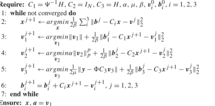
Algorithm 1 Compressive deconvolution SDMM-based algo-rithm.
Require: C1= 9−1H,C2= IN,C3= H ,α,µ,β,v0i,b0i,i= 1,2,3
1: while notconverged do 2: xj+1← argmin x 1 2β P3 ikbj− Cix− vjk22 3: vj1+1← argmin v1 kv1k+ 1 2βkb j 1− C1xj+1− vj1k22 4: vj2+1← argmin v2 αkv2kpp+2β1kb j 2− C2xj+1− vj2k22 5: vj3+1← argmin v3 1 2µky − 8C3v3k+2β1kb j 3− C3xj+1− vj3k22 6: bji+1= bji+ Cixj+1− vji+1,j= 1,2,3 7: end while Ensure: x,a= v1 hk+1= [(Xk+1P )tXk+1P+ γ In]−1[(Xk+1P )t9ak+1+ γ h0] (7) where In∈ Rnis the identity matrix. Based on the model
refor-mulation in (3), the analytical solution for estimating the PSF only requires the inversion of an n × n (the size of the PSF ker-nel) matrix instead of an N × N (the size of the TRF) matrix. The computational cost is thus considerably reduced. More de-tails about the practical implementation of the analytic solution in (7)can be found in Appendix B.
The proposed CSBD algorithm is summarized in Algo-rithm 2.
Algorithm 2 Compressive semi-blind deconvolution algorithm. Input: h0,α,µ,β,γ
1: while notconverged do
2: xk+1,ak+1← hk ⊲ updatexk+1,ak+1usingAlgorithm 1
3: hk+1← xk+1,ak+1 ⊲ updatehk+1using(7)
4: end while Output: x,a,h
3. Results
In this section, the performance of the proposed compressive semi-blind deconvolution method are evaluated on both simu-lated and experimental data sets.
3.1. Simulated US data
To get a quantitative insight about the algorithm perfor-mance, we first address the restoration of TRF, RF image and PSF on simulated US data where the degradation process (e.g., the variance of the additive Gaussian noise and the PSF) is known. To be in consistent with the direct model and regular-izations we proposed in this paper, we simulated the envelope US image with a 2D convolution between the TRF and a 7 × 7 spatially invariant Gaussian PSF of variance 2. The TRF sized of 300 × 300 was generated by assigning the scatterers random amplitudes following a given distribution, weighted by a car-toon image named by mask hereafter. A Laplacian distribution has been employed and the mask has been hand drawn to sim-ulate four different regions with different echogenicities. The resulting TRF and US image (plotted in B-mode) are shown in
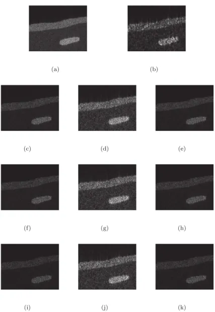
Fig. 1.SimulatedUSimageanditscompressiveblinddeconvolutionresultsforaSNRof40dB.(a)Originaltissuereflectivityfunction,(b)simulatedB-modeUS image,(c),(f),(i)resultsusingCDwiththetruePSFforCSratiosof0.8,0.6and0.4,(d),(g),(j)resultsusingCDwithapre-estimatedPSFforCSratiosof0.8,0.6 and0.4,(e),(h),(k)resultsusingCSBDforCSratiosof0.8,0.6and0.4.
were obtained by projecting the US images onto an orthogo-nal structurally random matrix (SRM) [34]and were degraded by an additive Gaussian noise corresponding to an SNR of 40 dB.
Based on the simulated US image in Fig. 1(b), an initial guess of the PSF was estimated using the algorithm in [16], shown in Fig. 2(b). Fig. 1(c)–(k) show a series of TRF recon-struction results using the SDMM-based CD algorithm given in
Algorithm 1with the known PSF, the SDMM-based CD with the initial estimated PSF and the proposed CSBD approach for CS ratios running from 0.4 to 0.8. We have also displayed the estimated PSFs in Fig. 2(c)–(e).
To evaluate the results quantitatively, we hereby employed two metrics: the standard peak signal-to-noise ratio (PSNR) and the Structural Similarity (SSIM) [35].
PSNR is defined as
PSNR= 10log10
N L2
k x − ˆx k2 (8)
where x and ˆx are the original and reconstructed images, N stands for the number of pixels in the image and the constant L represents the maximum intensity value in x.
SSIM, extensively used in US imaging, is defined as
SSIM= (2µxµxˆ+ c1)(2σxxˆ+ c2) (µ2
x+ µ2xˆ+ c1)(σx2+ σxˆ2+ c2)
(9) where x and ˆx are the original and reconstructed images, µx,
µxˆ, σx and σxˆ are the mean and variance values of x and ˆx,
σxxˆ is the covariance between x and ˆx; c1= (k1L)2and c2=
(k2L)2are two variables aiming at stabilizing the division with
weak denominator, L is the dynamic range of the pixel-values and k1, k2are constants. In this paper, L was set to 1, k1to 0.01
and k2to 0.03.
Table 1 regroups the PSNRs obtained with the proposed method, with SDMM-based CD algorithms using the known PSF (denoted as CD_true) and with SDMM-based CD
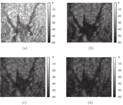
algo-Fig. 2.EstimatedPSFsofCSBD.(a)TruePSF,(b)estimatedPSFusinganexistingmethod[16],(c),(d),(e) estimatedPSFofCSBDforCSratiosof0.8,0.6 and 0.4.
Table 1
QuantitativeassessmentforsimulatedUSdata.
Methods CS ratios PSNRx SSIM PSNRh
CD_true 80% 29.29 80.10 – 60% 28.57 78.14 40% 27.07 73.91 20% 25.29 61.07 CD 80% 22.32 52.04 21.36 60% 22.33 50.51 40% 22.49 49.66 20% 22.72 45.76 CSBD 80% 28.55 80.03 44.74 60% 27.31 77.35 45.24 40% 26.87 73.22 44.68 20% 25.01 58.36 41.59
rithms using the initially estimated PSF for four CS ratios from 0.2 to 0.8. In each case, the reported PSNRs are the mean val-ues of 10 experiments.
3.2. In vivo US data
In this section, we tested our proposed method with an
in vivo image. The image (sized by 250 × 180) shown in
Fig. 3(a) was acquired with a 20 MHz single-element US probe and corresponds to part of a mouse kidney. In order to fit the compressive deconvolution framework, the measurements with CS ratios of 0.8, 0.6 and 0.4 were obtained by projecting the RF image onto the SRM and by further degradation with an addi-tive Gaussian noise corresponding to an SNR of 40 dB. Similar to the simulation results, the initial PSF in Fig. 4was estimated from the data using the method presented in [16]. Fig. 3 dis-plays the TRF reconstruction results of the proposed method and Fig. 4presents the corresponding PSFs.
3.3. Results’ discussion
We may firstly remark from the results on the simulated data in Fig. 1 and the quantitative metrics in Table 1 that the pro-posed CSBD ourperforms the non-blind CD method with an
Fig. 3. Results on in vivo data. (a) Original US image, (b)–(d) reconstruction results using CSBD for CS ratios of 0.8, 0.6 and 0.4, obtained for p = 1.5.
Fig. 4. Estimated PSFs with in vivo data. (a) Initial guess of PSF, (b)–(d) reconstruction results using CSBD for CS ratios of 0.8, 0.6 and 0.4.
initial guess of PSF. Moreover, the TRF reconstruction and PSF estimation of CSBD are very close to non-blind CD with the true PSF, which means that the algorithm converges to a crit-ical point which may be close to the global minimizer in this case. We emphasize that CSBD is in fact an algorithm to a non-convex minimization problem, and the convergence largely depends on the hyperparameters. In this study, we manually tuned these hyperparameters including the number of iterations to get the best results. For this set of hyperparameters, the
re-construction took around 9 minutes for the simulated image and 5 minutes for the in vivo data on the MacBook Air with 2.2 GHz Intel Core i7 and 8 GB RAM.
With the in vivo data, in the absence of TRF and PSF ground truth thus avoiding the computation of quantitative metrics, we can visually appreciate the contrast improvement of TRF recon-structions in Fig. 3(c), (d) compared to the original US image in Fig. 3(a). We may also observe from Fig. 4that the PSFs cor-responding to the in vivo data do not follow a Gaussian shape
as we simulated in Fig. 2, especially in the axial direction. This is in fact a typical US PSF, shown as [36]. With a relatively good initial guess of the PSF in Fig. 4(a), our proposed CSBD method can preserve the shape and calibrate the accuracy of the PSF at the same time.
4. Conclusions
The main objective of this paper is to propose an algo-rithm dedicated to reconstruct enhanced ultrasound images from compressed measurements with an unknown PSF, namely compressive semi-blind deconvolution. Compared to the non-blind compressive deconvolution method, the proposed method can achieve better reconstructions on both TRF and PSF. In addition to more validations with experimental data, our fu-ture work will also include the consideration of the parametric model of US PSF, to incorporate the prior information on its shape. Moreover, some existing non-convex optimization tech-niques with convergence guarantee, such as coordinate descent, would be of great interest to this problem.
Conflict of interest statement
There is no conflict of interest for this article. Appendix A
For the purpose of online PSF estimation, we write the con-volution model as below [37]:
r= XP h + n (10)
where r, h, n are the observation, the PSF and the noise in vec-tor forms respectively, r, n ∈ RN, h ∈ Rn. We should note that
in practical situations the size of the PSF is much smaller than the image size, i.e. n << N . X ∈ RN×N is the BCCB matrix representing the original image x and P ∈ RN×n is a matrix defined to extend h to N . Let us denote the size of x and H x as N = S × T , and the size of the PSF kernel h as n = s × t .
X has exactly the same structure as H , classically used in deconvolution problems. The matrix P can be written as
P =
" P′ ° #
where ° ∈ RS(T−t)×nis a zero matrix and P′∈ RSt×nhas the following structure P′= Is Os . . . Os O(S−s)s O(S−s)s . . . O(S−s)s Os Is . . . Os O(S−s)s O(S−s)s . . . O(S−s)s .. . ... . .. ... Os Os . . . Is O(S−s)s O(S−s)s . . . O(S−s)s
where Os represents a zero square matrix of size s × s and
O(S−s)s is a zero matrix of size (S − s) × s, Is is an identity
square matrix of size s × s.
Appendix B
In Section2, the analytical solution for PSF estimation is hk+1= [(Xk+1P )tXk+1P+ γ In]−1(Xk+1P )t9a (11)
To simplify the notations, we will ignore the iteration num-ber k and denote 9a by z. The key to solve this equation is to find an efficient way to compute (XP )tXP and (XP )tz.
Firstly, for the term of (XP )tz, Xt is actually the BCCB
ma-trix of the transformed x. Let us denote the transformed x by x′. Xtz is then the convolution between x′ and z. While x repre-sents the 2D image x2Din a vectorized version, x′corresponds
to the transformed 2D image x′2D. We define the pixels of x in 2D by: x2D= x11 x12 x13 . . . x1T x21 x22 x23 . . . x2T x31 x32 x33 . . . x3T .. . ... ... . .. ... xS1 xS2 xS3 . . . xST
The transformation from x2Dto x′2D usually includes flips
both in horizontal and vertical directions. However, the exact details of these flips depend also on the way the convolution product is defined, including its boundary conditions and the way the full convolution product is cropped to the size of the original image. Hereafter we will detail the transformation in the case of circular convolution with periodic boundary exten-sions, and we consider the center part of the full convolution. Thus x2Dcan be obtained by flipping x twice: the first row to
the last second and first column to the last second, which gives
x′2D= x(S−1)(T −1) x(S−1)(T −2) . . . x(S−1)1 x(S−1)T x(S−2)(T −1) x(S−2)(T −2) . . . x(S−2)1 x(S−2)T .. . ... . .. ... ... x1(T −1) x1(T −2) . . . x11 x1T xS(T−1) xS(T−2) . . . xS1 xST
According to the analysis on P above, Ptmultiplying a vec-tor is actually equivalent to choosing several elements from a vector. In our case, Ptaims picking up the first s elements from every S elements until we get n elements.
Secondly, concerning the term PtXtXP, its result is actually
a matrix of size n × n. To avoid constructing the big matrix P or Xduring implementation, we can find a way to compute these n × n elements instead.
Let us denote U = XtX, U is a symmetric matrix following the structure: U= U1 U2 U3 . . . UT U2 U1 U2 . . . UT−1 U3 U2 U1 . . . UT−2 .. . ... ... . .. ... UT UT−1 UT−2 . . . U1
where Ui(i= 1, 2...T ) is a matrix of size S × S. Let us analyse
the elements in this relative small matrix.
We know that every column in X is a transformed x. This kind of transformation includes circulation both in horizontal
and vertical directions. Let us denote the image which is cir-culated i times in horizontal direction and j times in vertical direction as x(ij )2D. Take an example, x(12)2D is equal to
x(12)= x(S−1)T x(S−1)1 x(S−1)2 . . . x(S−1)(T −1) xST xS1 xS2 . . . xS(T−1) x1T x11 x12 . . . x1(T −1) .. . ... ... . .. ... x(S−2)T x(S−2)1 x(S−2)2 . . . x(S−2)(T −1)
As a result, every element in XtX is an inner product be-tween two x(ij )(vectorized image x(ij )
2D). Now we can present
every detail of Ui. Here we use x(ij )as the vectorized image.
Ui=
x(00)x(i0) x(00)x(i1) . . . x(00)x(i(S−1)) x(01)x(i0) x(01)x(i1) . . . x(01)x(i(S−1))
.
.. ... . .. ... x(0(S−1))x(i0) x(0(S−1))x(i1) . . . x(0(−1)S)x(i(S−1))
As we can see, Ui is also a symmetric matrix. Moreover,
since x00xij = x00xi(S−j ), there are several elements with the same values even in the same row.
After understanding every detail about the XtX, now we can try to choose several elements out of the matrix to get the final result of PtXtXP. According to the definition of P we men-tioned before, the structure of PtXtXP can be written as
PtXtXP = U1′ U2′ U3′ . . . Ut′ U2′ U1′ U2′ . . . Ut−1′ U3′ U2′ U1′ . . . Ut−2′ .. . ... ... . .. ... Ut′ Ut′−1 Ut′−2 . . . U1′ where Ui′∈ Rs×sis Ui′=
x(00)x(i0) x(00)x(i1) . . . x(00)x(i(s−1)) x(01)x(i0) x(01)x(i1) . . . x(01)x(i(s−1))
..
. ... . .. ...
x(0(s−1))x(i0) x(0(s−1)x(i1) . . . x(0(s−1))x(i(s−1))
In conclusion, an efficient way to solve PtXtXP is to com-pute the s × s matrix Ui′. Since PtXtXP is symmetric, we will need only to compute Ui′ (i = 1, 2, .., t). Moreover, for each and Ui′, only the calculations of x00xij (j= 0, 1, ...s − 1) are
required, the computational cost is thus further reduced. References
[1]Friboulet D,Liebgott H,Prost R.CompressivesensingforrawRF sig-nalsreconstructioninultrasound.In:Ultrasonicssymposium,IUS.IEEE; 2010.p. 367–70.
[2]Quinsac C,Basarab A,Girault J-M,Kouamé D.Compressedsensingof ultrasoundimages:samplingofspatialandfrequencydomains(regular paper).In:IEEEworkshoponsignalprocessingsystems.IEEE;2010. p. 231–6.
[3]Quinsac C,Basarab A,Gregoire J-M,Kouamé D.3Dcompressed sens-ingultrasoundimaging(regularpaper).In:IEEEinternationalultrasonic symposium.IEEE;2010.p. 363–6.
[4]Achim A,Buxton B,Tzagkarakis G,Tsakalides P.Compressivesensing forultrasoundRFechoesusinga-stabledistributions.In:2010annual in-ternationalconferenceoftheIEEEengineeringinmedicineandbiology society.IEEE;2010.
[5]Chernyakova T,Eldar Y.Fourier-domainbeamforming:thepathto com-pressedultrasoundimaging.IEEETransUltrasonFerroelectrFreqControl 2014;61(8):1252–67.
[6]Lorintiu O,Liebgott H,Alessandrini M,Bernard O,Friboulet D. Com-pressed sensing reconstruction of 3D ultrasound data using dictio-nary learning and line-wise subsampling. IEEE Trans Med Imaging 2015;34(12):2467–77.
[7]Jin KH,Han YS,Ye JC.CompressivedynamicapertureB-mode ultra-soundimagingusingannihilatingfilter-basedlow-rankinterpolation.In: 2016IEEE13thinternationalsymposiumonbiomedicalimaging;2016. p. 1009–12.
[8]Besson A,Carrillo RE,Bernard O,Wiaux Y,Thiran JP.Compressed delay-and-sumbeamformingforultrafastultrasoundimaging.In:2016IEEE internationalconferenceonimageprocessing;2016.p. 2509–13.
[9]Liu J, He Q, Luo J. A compressed sensing strategy for syn-thetictransmitapertureultrasound imaging.IEEETransMedImaging 2017;36(4):878–91.
[10]Schiffner MF, Schmitz G. Fast compressive pulse-echo ultrasound imaging using random incident sound fields. J Acoust Soc Am 2017;141(5):3611.
[11] Liu J, He Q, Luo J. Compressed sensing based synthetic trans-mit aperture imaging: validation in a convex array configura-tion. IEEE Trans Ultrason Ferroelectr Freq Control 2017;PP(99):1.
https://doi.org/10.1109/TUFFC.2017.2682180.
[12]Candès EJ,Wakin MB.Anintroductiontocompressivesampling.IEEE SignalProcessMag2008;25(2):21–30.
[13] Quinsac C, Basarab A, Kouamé D. Frequency domain compressive samplingfor ultrasoundimaging. AdvAcoustVib, AdvAcoustSens, Imag, Signal Process2012;12:1–16. http://www.hindawi.com/journals/ aav/2012/231317/.
[14]Schiffner MF,Schmitz G.Fastpulse-echoultrasoundimagingemploying compressivesensing.In:2011IEEEinternationalultrasonicssymposium. IEEE;2011.p. 688–91.
[15]Liebgott H, Prost R, Friboulet D.Pre-beamformed RF signal recon-structioninmedicalultrasoundusingcompressivesensing.Ultrasonics 2013;53(2):525–33.
[16]Michailovich OV, Adam D. A novel approach to the2-D blind de-convolution probleminmedicalultrasound.IEEE TransMedImaging 2005;24(1):86–104.
[17]Jirik R,Taxt T.Two-dimensionalblindBayesiandeconvolutionof med-ical ultrasound images.IEEETransUltrason Ferroelectr FreqControl 2008;55(10):2140–53.
[18]Zhao N, Basarab A, Kouamé D, Tourneret J-Y. Joint segmentation and deconvolutionofultrasoundimagesusinga hierarchicalBayesian modelbasedongeneralizedGaussianpriors.IEEETransImageProcess 2016;25(8):3736–50.
[19]Chen Z,Basarab A,Kouamé D.Compressivedeconvolutioninmedical ultrasoundimaging.IEEETransMedImaging2016;35(3):728–37.
[20]Ma J,LeDimet F-X.Deblurringfromhighlyincompletemeasurements forremotesensing.IEEETransGeosciRemoteSens2009;47(3):792–802.
[21]Xiao L,Shao J,Huang L,Wei Z.Compoundedregularizationandfast algorithmforcompressivesensingdeconvolution.In:2011sixth interna-tionalconferenceonimageandgraphics.IEEE;2011.p. 616–21.
[22]Zhao M, Saligrama V.Oncompressed blindde-convolutionoffiltered sparse processes.In:2010IEEEinternational conferenceon acoustics speechandsignalprocessing.IEEE;2010.p. 4038–41.
[23]Amizic B,Spinoulas L,Molina R,Katsaggelos AK.Compressiveblind imagedeconvolution.IEEETransImageProcess2013;22(10):3994–4006.
[24]Bahmani S, Romberg J. Compressivedeconvolution in random mask imaging.IEEETransComputImag2015;1(4):236–46.
[25]Taxt T, Strand J. Two-dimensional noise-robust blind deconvolution of ultrasound images. IEEE Trans Ultrason Ferroelectr Freq Control 2001;48(4):861–6.
[26]Michailovich O,Tannenbaum A.Blinddeconvolutionofmedical ultra-soundimages:aparametricinversefilteringapproach.IEEETransImage Process2007;16(12):3005–19.
[27]Chen Z,Basarab A,Kouamé D.Reconstructionofenhancedultrasound images from compressed measurements using simultaneous direction method of multipliers.IEEE Trans Ultrason Ferroelectr Freq Control 2016;63(10):1525–34.
[28]Chen Z,Basarab A,Kouamé D.Enhancedultrasoundimage reconstruc-tionusingacompressiveblinddeconvolutionapproach(regularpaper).In: IEEEinternationalconferenceonacoustics,speech,andsignalprocessing. IEEE;2017.
[29]Almeida MS,Almeida LB.Blindandsemi-blinddeblurringofnatural im-ages.IEEETransImageProcess2010;19(1):36–52.
[30]Yu C, Zhang C, Xie L. A blind deconvolution approach to ul-trasound imaging. IEEE Trans Ultrason Ferroelectr Freq Control 2012;59(2):271–80.
[31]Morin R,Bidon S,Basarab A,Kouamé D.Semi-blinddeconvolutionfor resolutionenhancementinultrasoundimaging.In:201320thIEEE inter-nationalconferenceonimageprocessing,ICIP.IEEE;2013.p. 1413–7.
[32]Repetti A,Pham MQ,Duval L,Chouzenoux E,Pesquet J-C.Euclidina taxicab:sparseblinddeconvolutionwithsmoothedregularization.IEEE SignalProcessLett2015;22(5):539–43.
[33]Wang Y,Yang J,Yin W,Zhang Y.Anewalternatingminimization al-gorithmfortotalvariation imagereconstruction. SIAMJImagingSci 2008;1(3):248–72.é
[34]Do TT,Gan L, Nguyen NH,Tran TD.Fastand efficientcompressive sensingusingstructurallyrandommatrices.IEEETransSignalProcess 2012;60(1):139–54.
[35]Wang Z,Bovik AC,Sheikh HR,Simoncelli EP.Imagequalityassessment: fromerrorvisibilitytostructuralsimilarity.IEEETransImageProcess 2004;13(4):600–12.
[36]Zhao N,Wei Q,Basarab A,Kouamé D,Tourneret J-Y.Blind deconvolu-tionofmedicalultrasoundimagesusingaparametricmodelforthepoint spreadfunction(regularpaper).In:IEEEinternationalultrasonics sympo-sium.IEEE;2016.p. 1–4.
[37] MorinR.Améliorationdelarésolutionenimagerieultrasonore.Toulouse, France.PhD:UniversitédeToulouse;2013.Thèsededoctorat,inFrench (November2013).
![Fig. 2. Estimated PSFs of CSBD. (a) True PSF, (b) estimated PSF using an existing method [16] , (c), (d), (e) estimated PSF of CSBD for CS ratios of 0.8, 0.6 and 0.4.](https://thumb-eu.123doks.com/thumbv2/123doknet/3016077.84745/6.892.198.683.137.739/estimated-psfs-csbd-estimated-existing-method-estimated-ratios.webp)